Assessment of Baseflow Estimates Considering Recession Characteristics in SWAT

Abstract

Baseflow is influenced by incoming groundwater to aquifers and is closely related to watershed characteristics. Understanding baseflow characteristics is of great importance to river ecosystems and water management. Baseflow estimation typically depends on the observed streamflow in gauged watersheds, but accurate predictions of streamflow through modeling can also be useful in estimating baseflow. However, uncertainty occurs in the baseflow estimation process when modeling streamflow. Therefore, the purpose of this study is to compare the method that is proposed by Arnold and Allen (Scenario I) to an improved recession prediction method where the alpha factor (baseflow recession coefficient) is recalibrated and is applied to SWAT (Scenario II). Although the differences between the results (NSE, R², RMSE, MAE, d) of Scenarios I and II were small regarding streamflow and recession, the Scenario II method more accurately reflected the recession characteristics than the Scenario I method. Furthermore, the Scenario II method was better in baseflow prediction than for the Scenario I method proposed by Arnold and Allen. Therefore, these outputs pave the way and contribute to an efficient method for water management in watersheds.

1. Introduction

Baseflow is the portion of streamflow that is delayed subsurface flow and generally maintained by groundwater discharge. Regardless of the specific climatic environment, its main features are tightly related to geological catchment properties [1,2,3,4]. Baseflow is the streamflow that constitutes the majority of the streamflow on a day when rain does not occur or has not occurred recently [5]. Understanding the baseflow process is important to deal with various water resources issues, such as water resources management strategies, low flow conditions assessment, hydrological modeling calibration, and water quality studies [6].

However, no direct approach exists for continuously measuring the variability of streamflow recession under different conditions and the corresponding baseflow, because the baseflow is usually affected by diverse climatological and geological factors, with considerable variations in spatio-temporality [7,8]. Therefore, many efforts have been developed for analyzing baseflow characteristics [9,10,11]. For example, the baseflow recession curve method [12] and the groundwater topology curve method [13] have been used as analysis methods, and software for separating baseflow and the direct runoff from streamflow has been developed [14,15]. Understanding the role of baseflow in streamflow processes is critical for the identification and quantification of groundwater storage and direct runoff [16]. For this reason, many studies associated with the analyses of the characteristics of baseflow in watersheds have been conducted using various methods: the recession curve displacement method [17], the curve-fitting method [18], and the water-table fluctuation method [19]. In addition, HYSEP (Hydrograph Separation Program) [20], PART, RORA [21], BFlow [22,23], and WHAT (Web-based Hydrograph Analysis Tool) [24,25] have been developed and widely employed for hydrograph analysis on a long-term basis.

The Bflow program, which uses a digital filtering method [26], was developed and commonly used to provide consistent baseflow separation results. An important role of the Bflow program is to calculate an alpha factor, which is a parameter that is related to groundwater recharge and baseflow changes in a watershed. The alpha factor is a direct index of baseflow response to change in recharge of the shallow aquifer. Brutsaert and Nieber [27] reported that the recession parameter ‘alpha factor’ is a function of physical watershed characteristics, including hydraulic conductivity.

It can affect the shape of streamflow hydrographs, as it is a sensitive parameter [28]. The alpha factor can be derived using the Bflow program reflecting the recession characteristics and used to separate the direct runoff and the baseflow from the predicted streamflow and then used in hydrological models, such as Soil and Water Assessment Tool (SWAT). Various hydrological models can be used to predict streamflow at watershed scales. The SWAT model has been widely used in many environmental, hydrological applications around the world [29,30,31]. SWAT can quantify changes in hydrologic responses, such as runoff, water quality, groundwater recharge, and soil erosion in a watershed for various scenarios [32]. For this reason, SWAT has been applied in many water resources management studies around the world. Furthermore, SWAT-Calibration and Uncertainty Programs (SWAT-CUP) makes it easy for SWAT users to complement the model to compensate for main outlet from the watershed.

They gave a guideline (baseflow filter program) to analyze baseflow from the site (https://swat.tamu.edu/software/baseflow-filter-program) while mentioning that groundwater (gw) files in SWAT are needed to calculate the alpha factor that is estimated through Bflow in order to improve prediction of baseflow. Its search algorithm is adopted from Arnold and Allen [22]. Because groundwater (gw) files in SWAT provide constant values of the alpha factor, it is necessary to calculate the baseflow alpha factor, reflecting the measured streamflow data of the watershed. Use of Bflow with the SWAT model can provide results that are significantly improved due to the fact that the ratio of surface runoff to baseflow is improved. The Bflow program determines the runoff/baseflow fraction in streamflow [16].

The SWAT model, however, contains many parameters, and it does not always take into account the physical characteristics of each hydrological element in estimating the parameters. Further, there is uncertainty in calibrating the model with a combination of many parameters. In other words, due to the limitations of the statistics used for streamflow calibration, SWAT calibration is often highly biased toward high flow, and therefore does not correctly reflect the recession characteristics. For this reason, the method that is proposed by Arnold and Allen [22] can cause errors in recession curve simulation and baseflow estimation.

Accordingly, the objective of this study is to compare the method proposed by Arnold and Allen (Scenario I) with a new approach proposed here. First, to improve the recession prediction, the alpha factor is recalibrated and applied in SWAT (Scenario II). Second, the baseflow, accounting for the recession characteristics, is analyzed by using simulated results of streamflow (Scenario I and Scenario II).

2. Materials and Methods

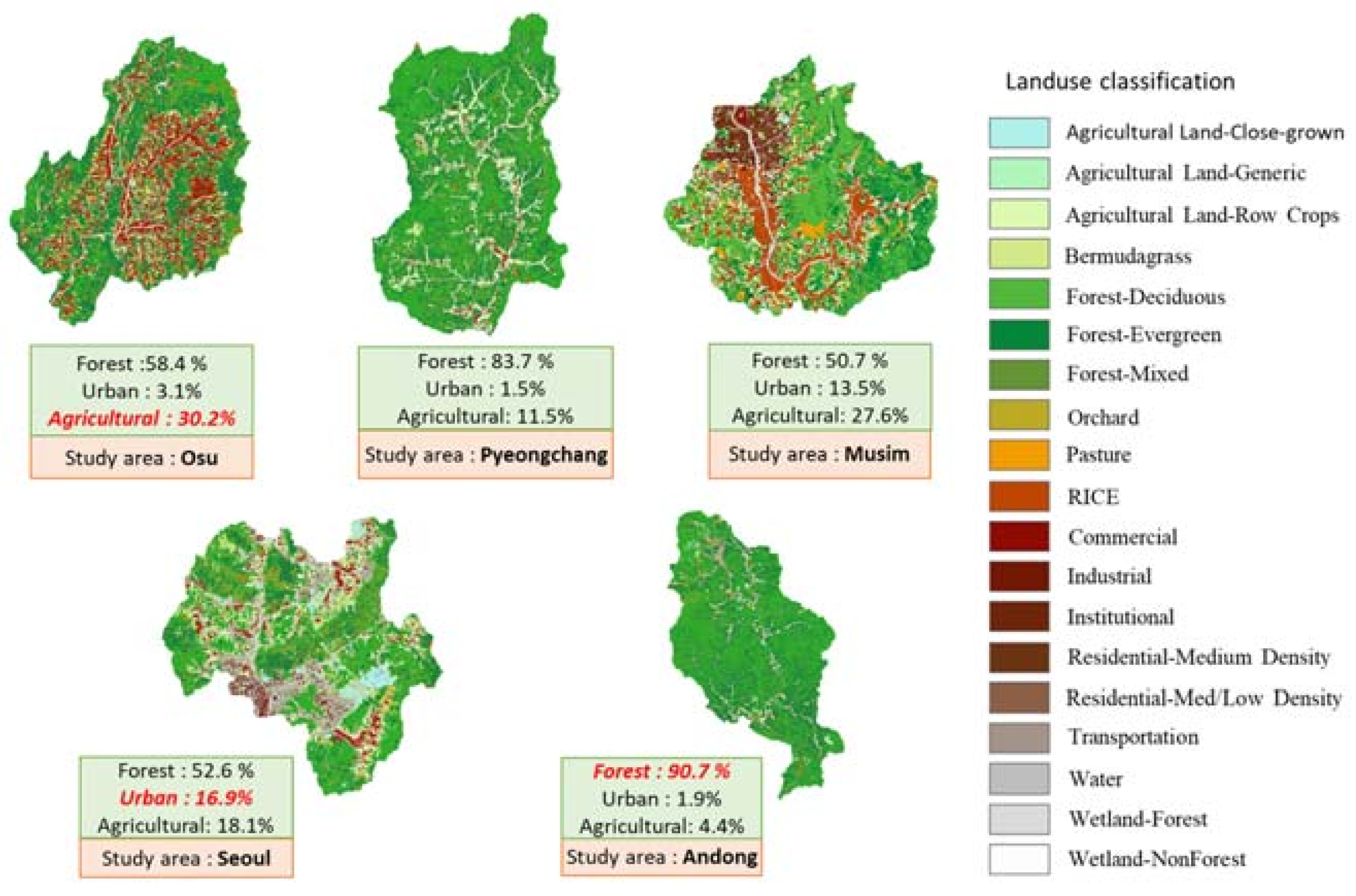
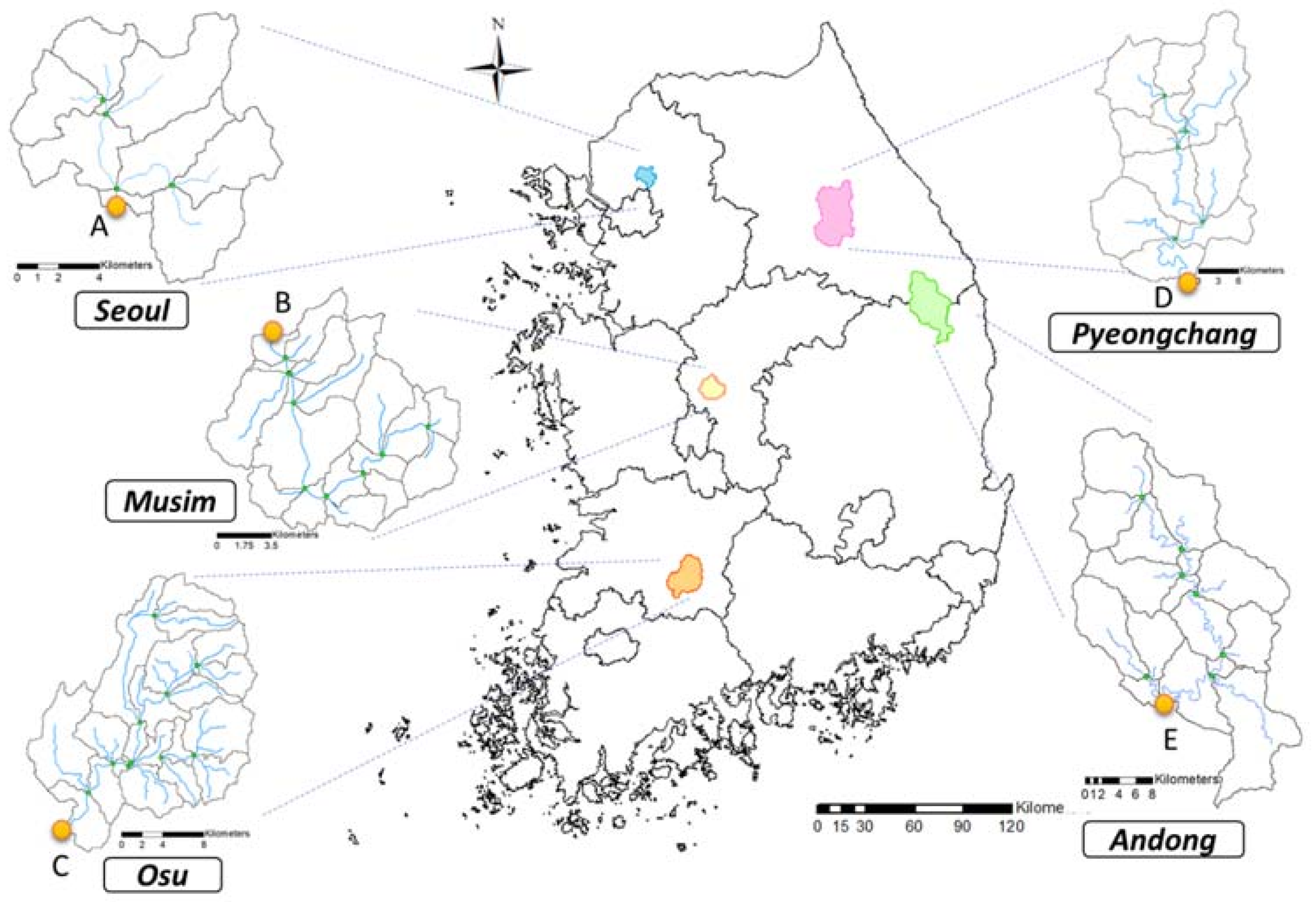
2.1. Study Area and Data

In this study, five study watersheds were selected, as shown in

Table 1. Characteristics of five study watersheds in South Korea.

Study Watershed	Periods	Area (km2)	Precipitation (mm/year)	Average Slope (%)	Highest Elevation (m)
Seoul	2008~2011	99.2	1751	9	600
Musim	2014~2016	156.7	869	11	595
Osu	2013~2016	392.0	1268	13	900
Andong	2010~2013	649.8	1237	27	1560
Pyeongchang	2007~2010	696.0	1310	21	1560

. The five watersheds have different conditions, such as land use, soil type, and watershed slope that might cause different recession characteristics. In order to evaluate baseflow prediction in SWAT, the alpha factor was calculated from the measured streamflow using Bflow and compared with the recalculated alpha factor from the simulated streamflow (calibrated) in SWAT for the five watersheds (Figure 1).

In order to consider and analyze the characteristics of recession, we investigated the streamflow stations that were included in the Water Management Information System (WAMIS) due to availability of continuous daily streamflow data, which is required for baseflow separation using the Bflow program. However, there is limited information on streamflow data provided by WAMIS in each study watershed, and the study period was different in each study watershed, as shown in Table 1.

In this study, the topographic data, which is input data for the SWAT model, were constructed using the Digital Elevation Model (DEM) of 30 m × 30 m resolution provided by the National Geographic Information Institute (http://www.ngii.go.kr/kor/main/main.do?rbsIdx=1), Republic of Korea. The reconnaissance soil map (1:25,000) provided by the Rural Development Administration (RDA) (http://soil.rda.go.kr/soil/index.jsp), Republic of Korea, was used as a base soil map. Climatic data used in the SWAT model are daily radiation (MJ/m), daily precipitation (mm), daily mean relative humidity (%), daily mean wind velocity (m/s), and daily maximum/minimum temperature (°C) from the KMA (Korea Meteorological Administration) (https://data.kma.go.kr/cmmn/main.do).

The distribution of land use in the study watersheds differs as shown in Figure 2. Among the five study watersheds, those with high forest density are located in Andong, urbanized watersheds are located in Seoul, and those in the Osu watershed are concentrated in agricultural watersheds.

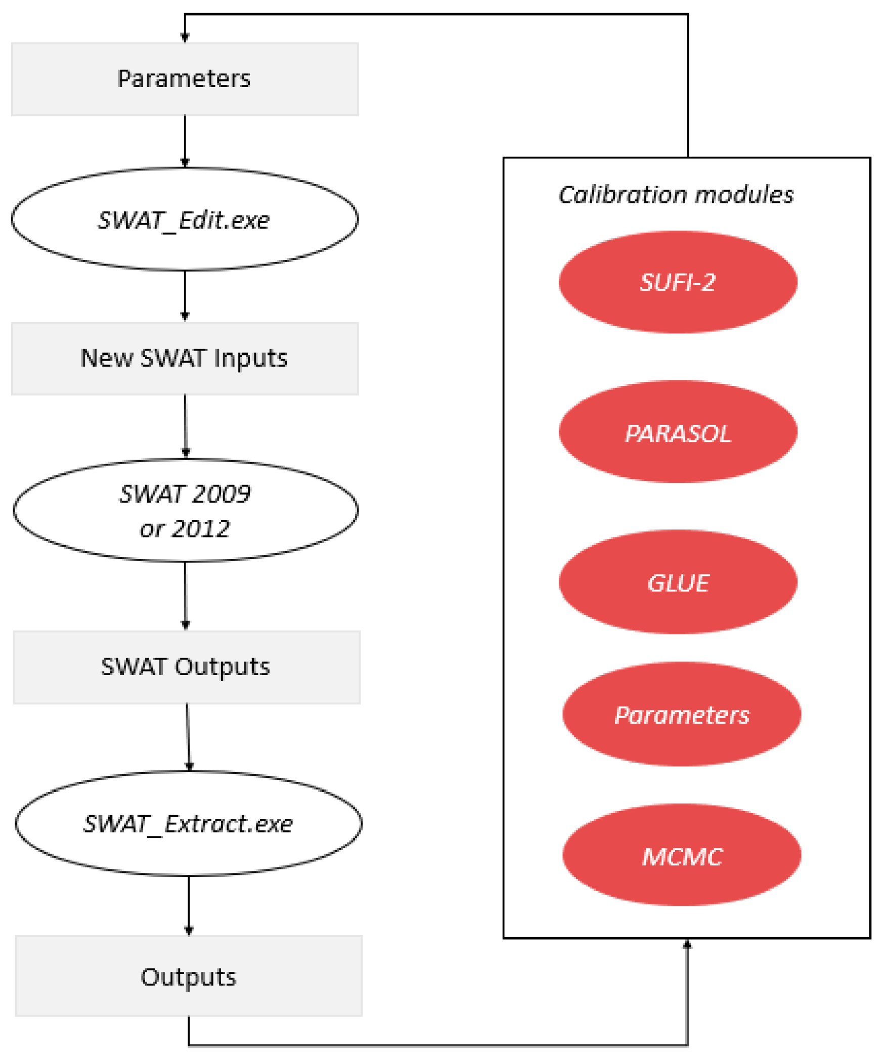
2.2. Description of SWAT and SWAT-CUP

SWAT is a semi-distributed rainfall-runoff model developed by the United States Department of Agriculture Research Service (USDA/ARS) [33,34]. The SWAT model is a continuous time model that operates on a daily time step and was developed to predict the impact of management on water, groundwater recharge, and sediment in large, complex watersheds. The model has physically based part and empirically based part, uses readily available inputs, is computationally efficient, and is able to continuously simulate long-term impacts. In particular, the model can quantitatively estimate changes in water quality due to changes in land use, climate, and vegetation.

Typically, SWAT requires data about watershed characteristics, including soil type, slope, land use, and meteorological data, including temperature, wind speed, precipitation, relative humidity, and solar radiation. SWAT performs the simulation based on the HRU (hydrological response unit) concept that uses a combination of land use, soil type, and watershed slope. The model simulates both hydrologic responses and water quality in subbasins, HRUs, and reaches using governing equations. For instance, the hydrologic process is simulated based on the water balance Equation (1).

$$S{W}_t=S{W}_0+{{\displaystyle \sum }}_{i=1}^t\left(R_{day}-E_a-W_{seep}-Q_{surf}-Q_{gw}\right)$$

(1)

where $S{W}_t$ is the final soil water content (mm H₂O), $S{W}_0$ is the initial soil water content (mm H₂O), t is time (days), $R_{day}$ is the amount of precipitation on day i (mm H₂O), $E_a$ is the amount of evapotranspiration on day i (mm H₂O), $W_{seep}$ is the amount of percolation and bypass flow exiting the soil profile bottom on day i (mm H₂O), $Q_{surf}$ is the amount of surface runoff on day i (mm H₂O), and $Q_{gw}$ is the amount of return flow on day i (mm H₂O).

The SWAT model contains many parameters related to rainfall runoff, and parameters that need to be calibrated to improve the accuracy of the prediction. Among the many parameters that are involved in the SWAT model, the alpha factor is the one of the most important parameters regarding the baseflow recession coefficient [35]. Recently, in order to incorporate various calibration modules into SWAT for automating calibration processes or uncertainty analysis, SWAT-calibration and uncertainty programs (SWAT-CUP) were developed (Figure 3).

SWAT-CUP includes the sequential uncertainty fitting algorithm (SUFI-2) [37], Parameter Solution (ParaSol) [38], Generalized Likelihood Uncertainty Estimation (GLUE) [39], Particle swarm optimization (PSO) [40], and Markov chain Monte Carlo (MCMC) [41]. Furthermore, by selecting the appropriate calibration algorithms corresponding to their needs, users can calibrate the SWAT model with observations at multiple outlets within a watershed. Moreover, users can manually adjust the period of observation that is used for calibration (e.g., the period of recession or flood).

In this study, calibration was performed using the sequential uncertainty fitting algorithm (SUFI-2), which has been used to optimize SWAT parameters in many studies [42,43,44].

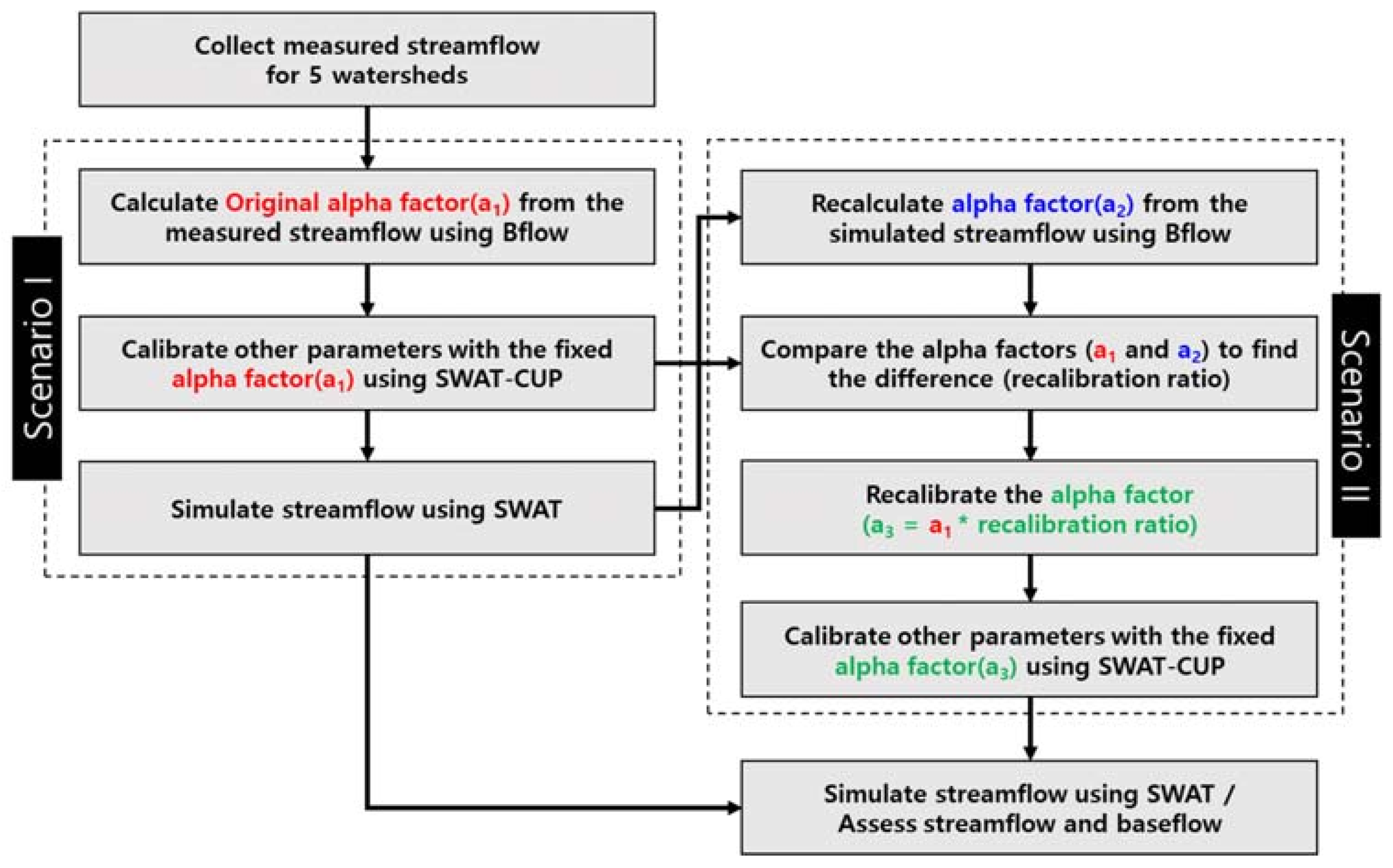
2.3. Alpha Factor Calculation and Baseflow Estimation Using Bflow

The recession provides crucial information on the flow of the stream and is closely related to baseflow. The SWAT model has a parameter (alpha factor) related to the recession, which represents the characteristics of the baseflow when simulating streamflow. The calculation of the alpha factor (a) is shown in Equation (2).

$$Q_t=Q_o{K}^t= Q_o^{}ex{p}^{-at}$$

(2)

$$a=-lnK$$

$Q_o$ is the streamflow at the starting point of the recession, $Q_t$ is streamflow at time t, and K is the recession index. In the case of the method that Arnold and Allen proposed, the alpha factor is calculated by using Bflow, and then the alpha factor is applied to groundwater (gw) files in SWAT. However, due to the fact that the calibration of SWAT is performed with a combination of many parameters, which can distort the results of simulating the overall streamflow, including the peak flow and the low flow, it is difficult for SWAT simulations to accurately reflect baseflow characteristics following calibration.

In this study, SWAT was calibrated using two methods (Scenario I, II), as shown in Figure 4, and the results (alpha factor and baseflow) from the two methods were compared. In order to compare the effectiveness of the two methods (Scenario I, II), five study watersheds (Seoul, Osu, Pyeongchang, Musim, and Andong) with different watershed characteristics were studied. In the case of Scenario I, the alpha factor was calculated from the measured streamflow using Bflow, and the alpha factor was applied to the SWAT model as a fixed parameter. The remaining parameters were calibrated by SWAT-CUP. This method has been commonly used for SWAT calibration. However, in this study, we found that the alpha factor was underestimated when reanalyzing the alpha factor from the simulated streamflow following calibration (refer to Section 3.1). Thus, as an alternative method, Scenario II was suggested that could adjust the alpha factor to improve baseflow prediction accuracy. In the case of Scenario II, the alpha factor was reanalyzed from the simulated streamflow (Scenario I) using Bflow and compared to the original alpha factor used in Scenario I to calculate the difference. The alpha factor was recalibrated based on the difference (recalibration ratio) and then applied in SWAT.

The Bflow filter can provide multiple passes through the filter (first pass, second pass, and third pass) allowing for users to select and use the desired number of passes to calculate the baseflow for the streamflow [45,46]. According to Eckhardt [2], the first or second pass results are typically used to separate baseflow using Bflow, since the baseflow contribution is relatively small for the third pass. Ahiablame et al. [6] constructed a regression equation to estimate baseflow within the state of Indiana for ungaged watersheds and calculated the baseflow that was used to create the equation using measured data from the first pass of Bflow. In this study, the first pass results were used. In order to analyze the baseflow reflecting the recession characteristics using Bflow, the baseflow was separated from the streamflow provided by the gage station. Moreover, the baseflow index (BFI), which indicates the contribution of baseflow in the flow, was calculated for each of the five research watersheds.

2.4. Evaluation of Streamflow and Baseflow Estimation from Scenario I and II

In this study, SWAT-CUP was used to calibrate the streamflow for the Seoul, Osu, Pyeongchang, Musim, and Andong watersheds. The alpha factor calculated by Bflow (Scenario I) and the recalibrated alpha factor to correctly take into account the recession (Scenario II) were used in SWAT-CUP as a fixed parameter to calibrate other parameters. After calibration using SWAT-CUP, the calibrated parameters, including the alpha factor were applied to SWAT to predict streamflow. The simulated streamflow and baseflow (separated by Bflow) were evaluated by comparing with the daily measured streamflow data for the five study watersheds. Nash-Sutcliffe efficiency coefficient (NSE) and determination coefficient (R²), root mean square error (RMSE), mean absolute error (MAE), and index of agreement (d) were used for SWAT model evaluation, and NSE, R², RMSE, MAE, and d can be calculated by using Equations (3–7). The R² measures the degree of collinearity between observations and simulations (Equation (3)). The NSE is a normalized statistic that gives the relative magnitude of the residual variance compared to the observed variance and is calculated by using Equation (4). An NSE value of “1” indicates perfect agreement between observations and simulations.

The advantage of the modified index of agreement is that the errors and differences are given their appropriate weighting and are not inflated by their squared values (Equation (4)). The modified index of agreement also varies from 0 to 1 with higher values indicating a better fit of the model [47,48]. Furthermore, several error indices are commonly used in model evaluation. These include MAE, and RMSE. These indices are valuable because they indicate error in the units (or squared units) of the constituent of interest, which aids in analysis of the results (Equations (6) and (7)). RMSE, and MAE values of 0 indicate a perfect fit [49]. Singh et al. [50] state that RMSE and MAE values less than half the standard deviation of the measured data may be considered as low, and either is appropriate for model evaluation. In this study, we compared baseflow estimates for each study watershed using NSE, R², RMSE, MAE, and d for comparison with the method that is proposed by Arnold and Allen.

$$R^2=\frac{{\left({{\displaystyle \sum }}_{i=1}^n\left(y_{obs,i}-{\overline{Y}}_{obs}\right)\left(y_{sim,i}-{\overline{Y}}_{sim}\right)\right)}^2}{{{\displaystyle \sum }}_{i=1}^n{(y_{obs,i}-{\overline{Y}}_{obs})}^2{{\displaystyle \sum }}_{i=1}^n{(y_{sim,i}-{\overline{Y}}_{sim})}^2}$$

(3)

$$NSE=1-\left[ \frac{{{\displaystyle \sum }}_{i=1}^n{\left(y_{obs,i}-y_{sim,i}\right)}^2}{{{\displaystyle \sum }}_{i=1}^n{\left(y_{obs,i}-{\overline{Y}}_{obs}\right)}^2} \right]$$

(4)

$$d=1-\left[\frac{{{\displaystyle \sum }}_1^n{\left(y_{obs,i}-y_{sim,i}\right)}^2}{{{\displaystyle \sum }}_1^n{\left(\left|y_{sim,i}-{\overline{Y}}_{obs}\right|+\left|y_{obs,i}-{\overline{Y}}_{obs}\right|\right)}^2}\right]$$

(5)

$$RMSE=\sqrt{\frac{{{\displaystyle \sum }}_1^n{\left(y_{sim,i}-y_{obs,i}\right)}^2}{n}}$$

(6)

$$MAE=\frac{1}{n}{\displaystyle \sum }_1^n\left|y_{sim,i}-y_{obs,i}\right|$$

(7)

where $y_{obs,i}$ is the observation, $y_{sim,i}$ is the simulation, ${\overline{Y}}_{obs}$ is the mean of the observations, ${\overline{Y}}_{obs}$ is the mean of the simulations, and n is the total number of observations.

3. Results

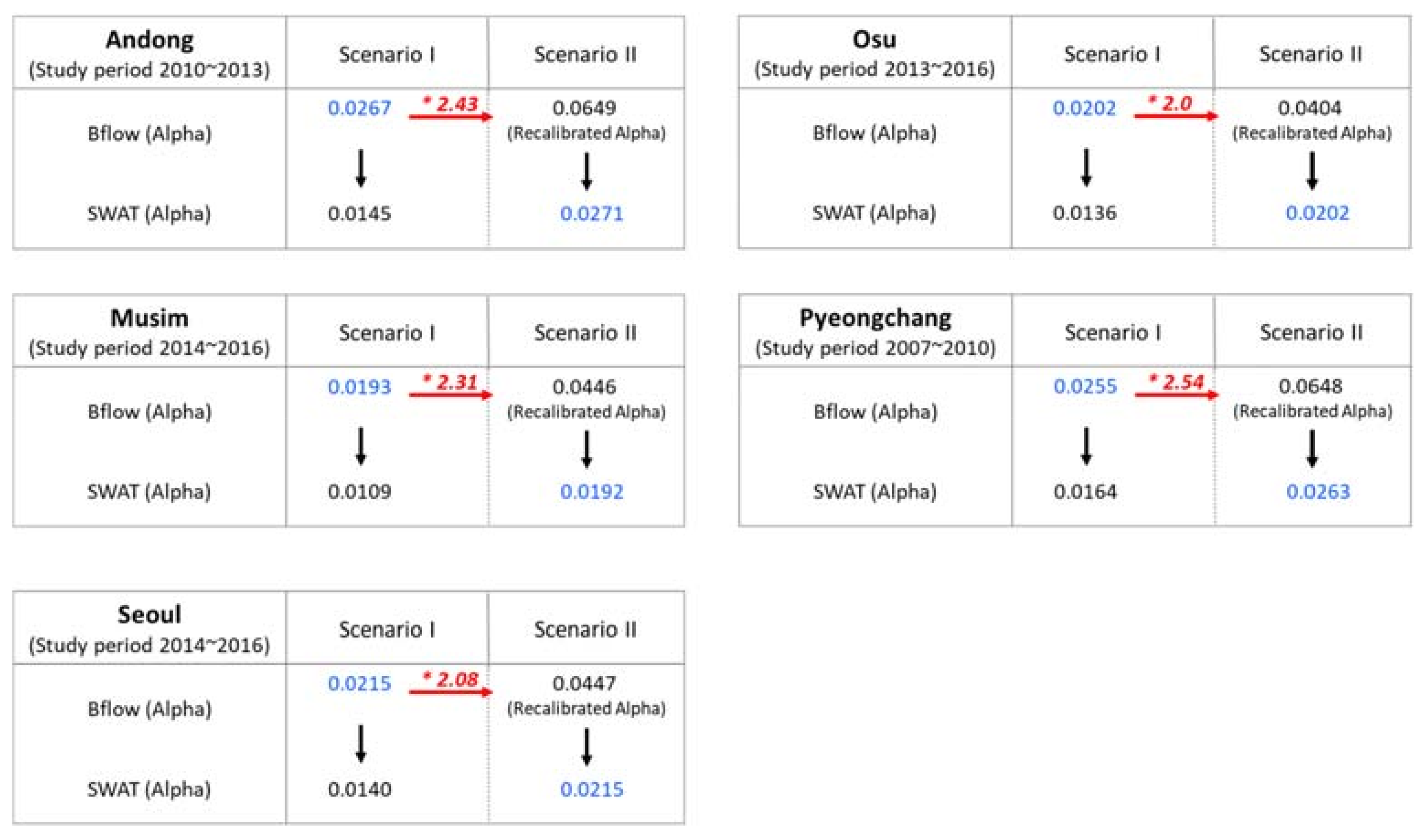
3.1. Comparison of Streamflow and Alpha Factor in Scenarios I and II

In this study, the alpha factor was estimated using Bflow to consider the recession characteristics in order to improve the accuracy in the SWAT model. The alpha factor, which is sensitive to the recession, was used as a fixed parameter in SWAT-CUP (Scenario I, proposed by Arnold and Allen [22]). The SWAT model was calibrated for measured streamflow in Seoul, Osu, Pyeongchang, Musim, and Andong basins. The calibration results are shown in

Table 2. Nash-Sutcliffe efficiency coefficient (NSE), determination coefficient (R²), root mean square error (RMSE), mean absolute error (MAE), and index of agreement (d) for Scenario I and Scenario II for streamflow for study watersheds.

Streamflow	Scenario I					Scenario II
	NSE	R2	RMSE	MAE	d	NSE	R2	RMSE	MAE	d
Seoul	0.573	0.762	21.454	5.000	0.790	0.579	0.763	21.382	4.978	0.793
Musim	0.974	0.974	1.040	0.845	0.970	0.989	0.989	0.258	0.161	0.995
Osu	0.666	0.672	13.771	4.265	0.898	0.666	0.673	13.240	4.041	0.901
Andong	0.546	0.549	30.500	10.500	0.837	0.547	0.558	30.470	10.390	0.840
Pyeongchang	0.562	0.564	34.060	11.708	0.840	0.567	0.569	33.850	11.340	0.845

. For Scenario II, the RMSE and MAE have a lower error rate than Scenario I. Also, d has more accurate results in Scenario II. The NSE were rated “Satisfactory” in the evaluation criteria of SWAT calibration (NSE > 0.5) (

Table 3. Reported performance ratings for NSE statistics [51].

Method	Value	Performance Rating
NSE	NSE ≥ 0.65	Very good
	0.54 ≤ NSE ≤ 0.65	Adequate
	NSE ≥ 0.50	Satisfactory

) based on guidance in Saleh et al. [51]. These NSE results show that Scenario I simulated streamflow well for the five study watersheds.

However, the recalculated alpha factor from the predicted streamflow (Scenario I) was underestimated due to the influence of other hydrologic parameters when the alpha factor that was calculated from Bflow was applied to SWAT-CUP (Figure 5). In order to properly reflect the calculated alpha factor from measured streamflow data, the alpha factor that was used in SWAT was recalibrated based on the difference between the alpha factor and the recalculated one. As shown in Figure 5, when calibrating using SWAT-CUP, it was necessary to recalibrate the alpha factor by multiplying the calculated alpha factor from the measured streamflow by two or a little more (difference or recalibration ratio) for the five study watersheds. Using this method, the recalculated alpha factors from the predicted streamflow (Scenario II) were similar to the alpha factor derived from the measured flow. When comparing the results of Scenario I and Scenario II, we can see that alpha factor for Scenario II more accurately reflects the recession than the alpha factor for Scenario I (Figure 5).

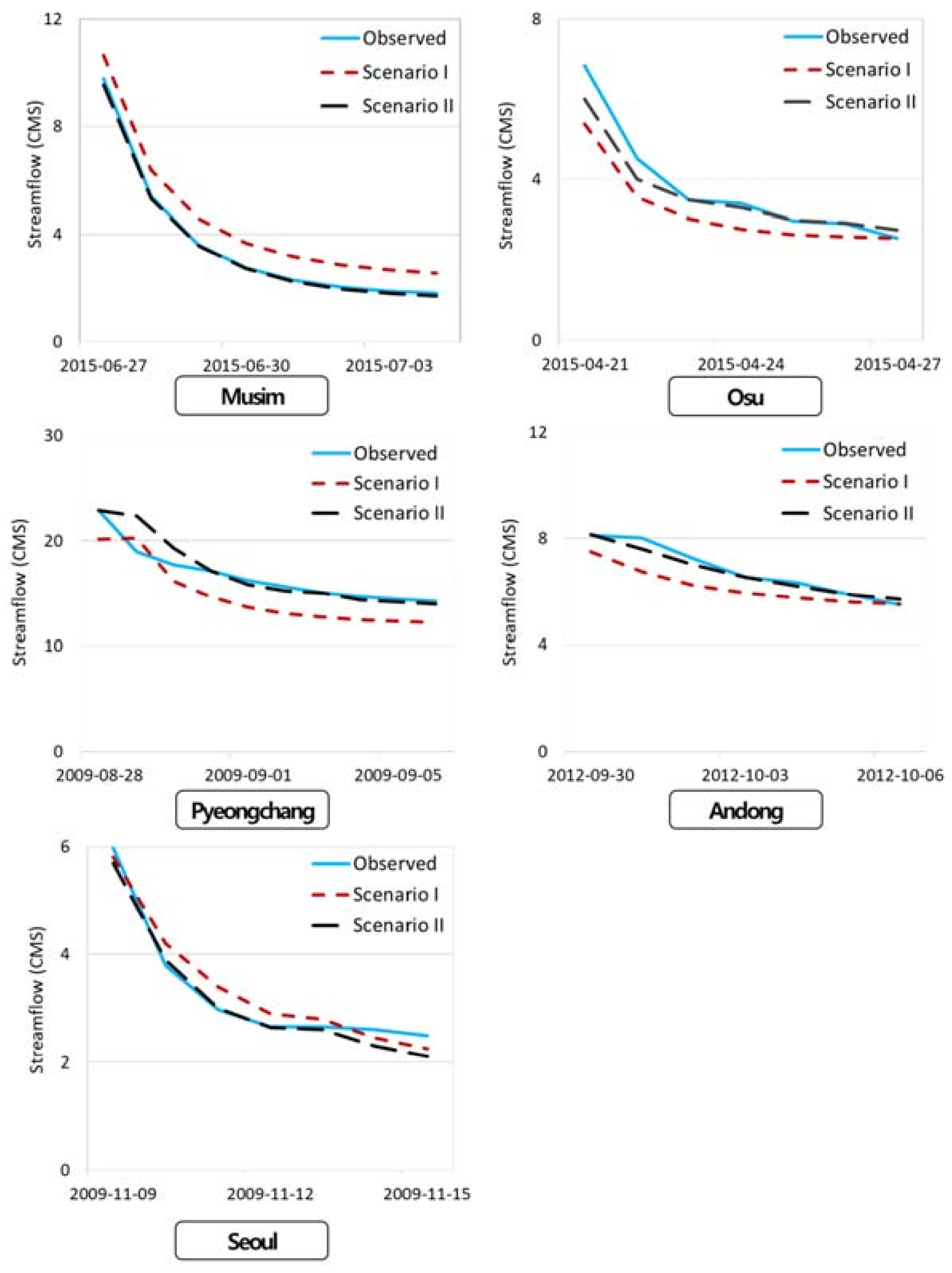
3.2. Comparison of Baseflow and Recession Estimates in Scenarios I and II

The recession curves were manually extracted from the simulated streamflow in Scenarios I and II. According to the SWAT performance rating shown in Table 3, the acceptable NSE and R² criteria ensuring satisfactory calibration are NSE > 0.5 and R² > 0.5 [52,53,54]. As shown in

Table 4. Comparison of streamflow recessions for Scenarios I and Scenarios II for study watersheds.

Recession Curve	Scenario I					Scenario II
	NSE	R2	RMSE	MAE	d	NSE	R2	RMSE	MAE	d
Seoul	0.534	0.723	30.585	7.920	0.766	0.537	0.725	30.480	7.751	0.768
Musim	0.969	0.971	1.089	0.893	0.981	0.988	0.989	0.288	0.169	0.992
Osu	0.745	0.752	18.031	5.233	0.916	0.746	0.752	18.010	5.202	0.917
Andong	0.604	0.639	34.276	12.066	0.834	0.606	0.640	34.183	12.026	0.836
Pyeongchang	0.696	0.794	38.180	13.206	0.876	0.704	0.797	37.678	12.711	0.881

, the effect of recession in Scenario II is simulated better than in Scenario I. In particular, the Musim watershed has the biggest difference (improvement) of NSE, RMSE, and MAE between Scenarios I and II among the five watersheds. The reason is that the average annual precipitation is the lowest (869 mm/year) in the Musim watershed compared to the other four study watersheds. This means that the baseflow had a greater effect than the peak flow effect when calibrating SWAT.

Figure 6 shows the observed and simulated streamflow recessions (extracted) for Scenarios I and II as an example of comparison of the recession curves. It shows that the recession simulations were in better agreement with the observed recessions for Scenario II when compared to Scenario I. Although trends in the recession curves are not consistent in each study watershed, Scenario II provides more accurate prediction for the recession curve than that of Scenario I in general.

BFI (Baseflow index) was analyzed based on measured streamflow of five study watersheds using Bflow. The BFI represents the characteristics of aquifers in the watershed and plays an important role in determining the characteristics of the runoff. The BFI results of five study watersheds were calculated (Seoul 0.52; Osu 0.58; Musim 0.68; Andong 0.58; Pyeongchang 0.60). Among the five study watersheds, Musim, where the baseflow rate is highest when compared to the direct runoff rate, has the largest value of BFI, while Seoul has the smallest value of BFI. The land use in Seoul is impervious due to urbanization relative to other watersheds. This means that the direct runoff ratio is larger than other watersheds.

Table 5. Comparison of baseflow results for Scenarios I and II after separation of baseflow from SWAT-modeled streamflow using Bflow.

Baseflow	Scenario I					Scenario II
	NSE	R2	RMSE	MAE	d	NSE	R2	RMSE	MAE	d
Seoul	0.479	0.853	5.449	2.397	0.738	0.503	0.853	5.324	2.387	0.758
Musim	0.902	0.932	0.512	0.384	0.961	0.982	0.987	0.156	0.143	0.996
Osu	0.509	0.511	3.159	2.134	0.824	0.586	0.589	2.900	2.051	0.863
Andong	0.622	0.689	6.057	4.657	0.904	0.627	0.691	6.022	4.067	0.906
Pyeongchang	0.788	0.791	6.473	4.524	0.934	0.810	0.811	6.134	4.179	0.946

shows the results obtained by separating the baseflow from streamflow using Bflow. Since the influence of low flow rate is bigger than that of the high flow rate, the result of Scenario II is more accurate than that of Scenario I on prediction of baseflow. The highest values of NSE, R², RMSE, MAE, and d were found for the Musim watershed for the baseflow results. In addition, the difference between Scenarios I and II of the Musim watershed was great. This is because the Musim watershed has less influence from precipitation than other watersheds as it has the lowest precipitation. This indicates that the influence of low flow is greater than the influence of specific high flow, such as during the flood season, and the low flow is sensitive to the baseflow.

However, in the Andong area, the difference between NSE and R² for Scenario I and Scenario II was small likely because the average slope of the Andong area is steepest at 27 (%), and it has the highest elevation, 1560 (m). Therefore, direct runoff is expected to have greater influence than that of baseflow. The baseflow is sensitive to time and space variations, and it is influenced by various conditions such as variability in weather or geography.

Thus, our findings show that if SWAT is calibrated for recession periods and baseflow with the alpha factor (Scenario II), streamflow recession, and baseflow were more accurately predicted. These findings indicate that the SWAT model with this new approach for baseflow estimation will be useful for planning of sustainable groundwater management.

4. Conclusions

In this study, we calculated alpha factors reflecting the characteristics of five study watersheds and analyzed baseflow when comparing the method proposed by Arnold and Allen (Scenario I) with a new approach proposed here (Scenario II). The method proposed by Arnold and Allen was used to calculate the alpha factor when considering the recession characteristics and applied in the SWAT model as Scenario I, and then the alpha factor was recalibrated to reflect recessions more precisely in SWAT in Scenario II. From the results, we found that the method that is proposed by Arnold and Allen could not more precisely reflect the alpha factor considering recession characteristics in SWAT. If the alpha factor was applied to the SWAT-CUP calibration after multiplying the calculated alpha factor from the measured streamflow data by approximately 2.0 (recalibration ratio) proposed in Scenario II of this study, baseflow prediction in SWAT could be improved taking account of the recession characteristics correctly. Although the differences between the results (NSE, R², RMSE, MAE, d) of Scenario I and Scenario II were small, the Scenario II method more accurately reflected the recession characteristics than the Scenario I method.

The baseflow analysis approach proposed in this study that considers recession characteristics can be used to validate and evaluate baseflow in other study watersheds. Since considering recession characteristics is important to baseflow analysis, the approach developed can be used not only in this study, but also in other studies regarding baseflow. These outputs will pave the way and contribute to the water management of watersheds in an efficient manner and help us to predict upstream runoff phenomenon with more accuracy.

Due to the lack of streamflow observation data in the study watersheds, only one alpha factor was applied to the entire watershed. Therefore, future studies should be conducted when considering the influence of the baseflow of each sub basin.

References

1. Hong, J.; Lim, K.J.; Shin, Y.; Jung, Y. Quantifying Contribution of Direct Runoff and Baseflow to Rivers in Han River System, South Korea. J. Korea Water Resour. Assoc. 2015, 48, 309–319. [Google Scholar] [CrossRef]
2. Eckhardt, K. A comparison of baseflow indices, which were calculated with seven different baseflow separation methods. J. Hydrol. 2008, 352, 168–173. [Google Scholar] [CrossRef]
3. Cherkauer, D.S.; Ansari, S.A. Estimating groundwater recharge from topography, hydrogeology, and land cover. Groundwater 2005, 43, 102–112. [Google Scholar] [CrossRef]
4. Santhi, C.; Allen, P.; Muttiah, R.; Arnold, J.; Tuppad, P. Regional estimation of baseflow for the conterminous United States by hydrologic landscape regions. J. Hydrol. 2008, 351, 139–153. [Google Scholar] [CrossRef]
5. Joo, S.W.; Park, Y.S.; Kim, J.G.; Heo, S.G.; Choi, J.D.; Lim, K.J. Estimation of BFI max value for accurate baseflow separation using WHAT system. J. Agric. Sci. Kangwon Natl. Univ. 2007, 18, 155–162. [Google Scholar]
6. Ahiablame, L.; Chaubey, I.; Engel, B.; Cherkauer, K.; Merwade, V. Estimation of annual baseflow at ungauged sites in Indiana USA. J. Hydrol. 2013, 476, 13–27. [Google Scholar] [CrossRef]
7. Lin, K.R.; Guo, S.L.; Zhang, W.H.; Liu, P. A new baseflow separation method based on analytical solutions of the Horton infiltration capacity curve. Hydrol. Process. 2007, 21, 1719–1736. [Google Scholar] [CrossRef]
8. Datta, A.R.; Bolisetti, T.; Balachandar, R. Automated linear and nonlinear reservoir approaches for estimating annual baseflow. J. Hydrol. Eng. 2011, 17, 554–564. [Google Scholar] [CrossRef]
9. Cheng, Q.B.; Chen, X.; Xu, C.Y.; Imjela, C.R.; Schulte, A. Improvement and comparison of like likelihood functions for model calibration and parameter uncertainty analysis within a Markow chain Monte Carlo scheme. J. Hydrol. 2014, 519, 2202–2214. [Google Scholar] [CrossRef]
10. Evenson, G.R.; Golden, H.E.; Lane, C.R.; D’Amico, E. Geographically isolated wetlands and watershed hydrology: A modified model analysis. J. Hydrol. 2015, 529, 240–256. [Google Scholar] [CrossRef]
11. Leta, O.T.; El-Kadi, A.I.; Dulai, H.; Ghazal, K. Assessment of climate change impacts on water balance components of Heeia watershed in Hawaii. J. Hydrol. Reg. Stud. 2016, 8, 182–197. [Google Scholar] [CrossRef]
12. Thomas, B.F.; Vogel, R.M.; Famiglietti, J.S. Objective hydrograph baseflow recession analysis. J. Hydrol. 2015, 525, 102–112. [Google Scholar] [CrossRef]
13. Sposito, G. Topological groundwater hydrodynamics. Adv. Water Resour. 2001, 24, 793–801. [Google Scholar] [CrossRef]
14. Jung, Y.; Shin, Y.; Won, N.; Lim, K.J. Web-Based Bflow system for the Assessment of Streamflow characteristics at National Level. Water 2016, 8, 384. [Google Scholar] [CrossRef]
15. Lim, K.J.; Park, Y.S.; Kim, J.G.; Shin, Y.C.; Kim, N.W.; Jeon, J.H.; Engel, B.A.; Kim, S.J.; Jeon, J.H. Development of Genetic Algorithm-Based Optimization Module in WHAT System for Hydrograph Analysis and Model Application. Comput. Geosci. 2010, 36, 936–944. [Google Scholar] [CrossRef]
16. Lee, J.; Park, Y.S.; Jung, Y.; Cho, J.; Yang, J.E.; Lee, G.; Kim, K.S.; Lim, K.J. Analysis of spatio-temporal changes in groundwater recharge and baseflow using SWAT and Bflow models. J. Korean Soc. Water Environ. 2014, 30, 549–558. [Google Scholar] [CrossRef]
17. Rutledge, A.T.; Mesko, T.O. Estimated Hydrologic Characteristics of Shallow Aquifer Systems in the Valley and Ridge, the Blue Ridge, and the Piedmont Physiographic Provinces Based on Analysis of Streamflow Recession and Base Flow; U.S. Geological Survey: Reston, VA, USA, 1996; pp. 1–58.
18. Molugaram, K.; Rao, G.S.; Shah, A.; Davergave, N. Chapter 5—Curve Fitting. In Statistical Techniques for Transportation Engineering; Butterworth-Heinemann: Woburn, MA, USA, 2017; pp. 281–292. [Google Scholar]
19. Healy, R.W.; Cook, P.G. Using groundwater levels to estimate recharge. Hydrogel. J. 2002, 10, 91–109. [Google Scholar] [CrossRef]
20. Sloto, R.A.; Crouse, M.Y. HYSEP: A Computer Program for Streamflow Hydrograph Separation and Analysis; No. 96–4040; U.S. Geological Survey Water-Resources Investigations Report; U.S. Geological Survey: Reston, VA, USA, 1996; pp. 1–54.
21. Rutledge, A. Computer Programs for Describing the Recession of Ground-Water Discharge and for Estimating Mean Ground-Water Recharge and Discharge from Stream-flow Records: Update; U.S. Geological Survey Water-Resources Investigations Report; U.S. Geological Survey: Reston, VA, USA, 1998; pp. 98–4148.
22. Arnold, J.G.; Allen, P.M. Automated Methods for Estimating Baseflow and Groundwater Recharge from Streamflow Records. J. Am. Water Resour. Assoc. 1999, 35, 411–424. [Google Scholar] [CrossRef]
23. Arnold, J.G.; Allen, P.M.; Muttiah, R.; Bernhardt, G. Automated Base Flow Separation and Recession Analysis Techniques. Groundwater 1995, 33, 1010–1018. [Google Scholar] [CrossRef]
24. Lim, K.J.; Engel, B.A.; Tang, Z.; Choi, J.; Kim, K.; Muthu, K.S.; Tripathy, D. Automated Web GIS Based Hydrograph Analysis Tool, WHAT 1. J. Am. Water Resour. Assoc. 2005, 41, 1407–1416. [Google Scholar] [CrossRef]
25. Yang, J.S.; Chi, D.K. Correlation Analysis between Groundwater Level and Baseflow in the Geum River Water-shed, Calculated Using the WHAT System. J. Eng. Geol. 2011, 21, 107–116. [Google Scholar] [CrossRef]
26. Chapman, T.G.; Maxwell, A.I. Baseflow Separation Comparison of Numerical Methods with Tracer Experiments. In Proceedings of the 23rd Hydrology and Water Resources Symposium, Hobart, Tasmania, Australia, 21–24 May 1996; Volume 96, pp. 539–545. [Google Scholar]
27. Brutsaert, W.; Nieber, J.L. Regionalized drought flow hydrographs from a mature glaciated plateau. Water Resour. 1977, 13, 637–643. [Google Scholar] [CrossRef]
28. Navarro, E.M.; Alegria, M.H.; Perez, S.M.; Hernandez, J.R.; Moctezuma, A.M.; Merlin, A.S. Hydrological modeling and climate change impacts in an agricultural semiarid region. Case study: Guadalupe river basin, Mexico. Agric. Water Manag. 2016, 175, 29–42. [Google Scholar] [CrossRef]
29. Mehran, N.; Christopher, O.; Robert, M. Pathogen transport and fate modeling in the upper Salem river watershed using SWAT model. J. Environ. Manag. 2015, 151, 167–177. [Google Scholar]
30. Lee, J.E.; Heo, J.H.; Lee, J.; Kim, N.W. Assessment of Flood frequency alteration by Dam construction via SWAT simulation. Water 2014, 9, 264. [Google Scholar] [CrossRef]
31. Ligaray, M.; Kim, H.; Sthiannopkao, S.; Lee, S.; Cho, K.H.; Kim, J.H. Assessment on Hydrologic Response by climate change in the Chao Phraya river basin, Thailand. Water 2015, 7, 6892–6909. [Google Scholar] [CrossRef]
32. Lee, J.; Park, Y.S.; Kum, D.; Jung, Y.; Kim, B.; Hwang, S.J.; Kim, H.B.; Kim, C.; Lim, K.J. Assessing the effect of watershed slopes on recharge/baseflow and soil erosion. Paddy Water Environ. 2014, 12 (Suppl. 1), S169–S183. [Google Scholar] [CrossRef]
33. Arnold, J.G. Spatial Scale Variability in Model Development and Parameterization. Ph.D. Thesis, Purdue University, West Lafayette, IN, USA, 1992; pp. 1–186. [Google Scholar]
34. Arnold, J.G.; Srubuvasan, R.; Muttiah, R.; Muttiah., R.S.; Williams, J.R. Large area hydrologic modeling and assessment, part I: Model development. J. Am. Water Resour. Assoc. 1998, 34, 73–89. [Google Scholar] [CrossRef]
35. Lee, G.; Shin, Y.; Jung, Y. Development of WEB-Based RECESS model for estimating baseflow using SWAT. Sustainability 2014, 6, 2357–2378. [Google Scholar] [CrossRef]
36. Abbaspour, K.C. SWAT-CUP4: SWAT Calibration and Uncertainty Programs—A User Manual; EAWAG Swiss Federal Institute of Aquatic Science and Technology: Dubendorf, Switzerland, 2011; pp. 1–103. [Google Scholar]
37. Abbaspour, K.C.; Yang, J.; Maximov, I.; Siber, R.; Bonger, K.; Mieleitner, J.; Zobrist, J.; Srinivasan, R. Modeling hydrology and water quality in the pre-alpine Thur watershed using SWAT. J. Hydrol. 2007, 332, 413–430. [Google Scholar] [CrossRef]
38. Van Griensven, A.; Meixner, T. Methods to quantify and identify the sources of uncertainty for river basin water quality models. J. Water Sci. Technol. 2006, 53, 51–59. [Google Scholar] [CrossRef]
39. Beven, K.J.; Binley, A.M. The future of distributed models: model calibration and uncertainty prediction. J. Hydrol. Process. 1992, 6, 273–298. [Google Scholar] [CrossRef]
40. Eberhart, R.; Kennedy, J. A New optimizer using particle swarm theory. In Proceedings of the Sixth International Symposium on Micro Machine and Human Science, Nagoya, Japan, 4–6 October 1995; pp. 39–43. [Google Scholar]
41. Kuczera, G.; Parent, E. Monte Carlo assessment of parameter uncertainty in conceptual catchment models: The Metropolis algorithm. J. Hydrol. 1998, 211, 69–85. [Google Scholar] [CrossRef]
42. Paul, S.; Cashman, M.A.; Szura, K.; Pradhanang, S.M. Assessment of nitrogen inputs into Hunt river by onsite wastewater treatment system via SWAT simulation. Water 2017, 9, 610. [Google Scholar] [CrossRef]
43. Gebiaw, T.A.; Engidasew, Z.T.; Bofu, Y.; Ian, D.R.; Jaehak, J. Streamflow and sediment yield prediction for watershed prioritization in the upper Blue Nile river basin, Ethiopia. Water 2017, 9, 782. [Google Scholar]
44. Gokhan, C.; Karim, C.A.; Izzet, O. Assessing the water-resource potential of Istanbul by using a soil and water assessment tool (SWAT) hydrological model. Water 2017, 9, 814. [Google Scholar]
45. Lyne, V.D.; Hollick, M. Stochastic Time-Variable Rainfall Runoff Modeling. In Proceedings of the Institute of Engineers Australia National Conference, Perth, Australia, 10–12 September 1979; pp. 89–92. [Google Scholar]
46. Schwartz, S.S.; Smith, B.; McGuire, M. Baseflow Signatures of Sustainable Water Resources; Final Report to the Hughes Center for Agroecology; Hughes Center for Agroecology: Queenstown, MD, USA, 2012. [Google Scholar]
47. Willmott, C.J.; Wicks, D.E. An empirical method for the spatial interpolation of monthly precipitation within California. Phys. Geogr. 1980, 1, 59–73. [Google Scholar]
48. Willmott, C.J. On the validation of models. Phys. Geogr. 1981, 2, 184–194. [Google Scholar]
49. Moriasi, D.N.; Arnold, J.G.; Van Liew, M.W.; Binger, R.L.; Harmel, R.D.; Veith, T.L. Model evaluation guidelines for systematic quantification of accuracy in Watershed simulations. Am. Soc. Agric. Biol. Eng. 2007, 50, 885–900. [Google Scholar]
50. Singh, J.; Knapp, H.V.; Demissie, M. Hydrologic Modeling of the Iroquois River Watershed Using HSPF and SWAT; ISWS CR 2004-08; Illinois State Water Survey: Champaign, IL, USA, 2004; pp. 1–24. [Google Scholar]
51. Saleh, A.; Arnold, J.; Gassman, P.W.A.; Huack, L.; Rosenthal, W.; Williams, J.; McFarland, A. Application of SWAT for the upper north Bosque river watershed. Am. Soc. Agric. Biol. Eng. 2000, 43, 1077–1087. [Google Scholar] [CrossRef]
52. Ramanarayanan, T.S.; Wiliams, J.R.; Dugas, W.A.; Hauck, L.M.; McFarland, A.M.S. Using APEX to Identify Alternative Practices for Animal Waste management. In Proceedings of the ASAE International Meeting, Minneapolis, MN, USA, 10–14 August 1997; pp. 97–2209. [Google Scholar]
53. Santhi, C.; Arnold, J.G.; Williams, R.; Dugas, W.A.; Srinivasan, R.; Hauck, L.M. Validation of the SWAT model on a large river basin with point and nonpoint sources. J. Am. Water Resour. Assoc. 2001, 37, 1169–1188. [Google Scholar] [CrossRef]
54. Van Liew, M.W.; Arnold, J.G.; Garbrecht, J.D. Hydrologic simulation on agricultural watershed: Choosing between two models. Trans. ASAE 2003, 46, 1539–1551. [Google Scholar] [CrossRef]
Figure 1. Locations of the five study watersheds (Seoul, Musim, Osu, Pyeongchang, Andong) in South Korea. Symbols and letters denote the locations of streamflow measurement stations.
Water 10 00371 g001
Figure 2. Land use of the five study watersheds (Seoul, Musim, Osu, Pyeongchang, Andong).
Water 10 00371 g002
Figure 3. Overview of Soil and Water Assessment Tool -Calibration and Uncertainty Programs (SWAT-CUP) for automated calibration of SWAT [36].
Water 10 00371 g003
Figure 4. SWAT application procedure for accurate prediction of hydrograph recession.
Water 10 00371 g004
Figure 5. Recalibration of alpha factor for the recession curve for five study watersheds. The values in red represent the differences between the alpha factors calculated from measured and simulated (calibrated) streamflow in Scenario I and the recalibration ratio applied in Scenario II. The blue color in Scenario I is a calculated alpha value by Bflow. The blue in Scenario II is a calculated Alpha value by Bflow after applying the recalibrated alpha to SWAT.
Water 10 00371 g005
Figure 6. Observed and simulated streamflow recessions for five study watersheds.
Water 10 00371 g006