Article

Near-Bed Monitoring of Suspended Sediment during a Major Flood Event Highlights Deficiencies in Existing Event-Loading Estimates

1
School of Civil Engineering, The University of Queensland, Brisbane, QLD 4072, Australia
2
The Port of Brisbane Pty Ltd., Brisbane, QLD 4178, Australia
*
Author to whom correspondence should be addressed.
Water 2018, 10(2), 34; https://doi.org/10.3390/w10020034
Submission received: 15 November 2017 / Revised: 16 December 2017 / Accepted: 17 January 2018 / Published: 23 January 2018

Abstract

:
Rates of fluvial sediment discharge are notoriously difficult to quantify, particularly during major flood events. Measurements are typically undertaken using event stations requiring large capital investment, and the high cost tends to reduce the spatial coverage of monitoring sites. This study aimed to characterise the near-bed suspended sediment dynamics during a major flood event using a low-cost approach. Monitoring nodes consisted of a total suspended sediment (TSS) logger, a single stage sampler, and a time-lapse camera for a total cost of less than US$420. Seven nodes were deployed across an elevation gradient on the stream bank of Laidley Creek, Queensland, Australia, and two of these nodes successfully characterised the near-bed suspended sediment dynamics across a major flood event. Near-bed TSS concentrations were closely related to stream flow, with the contribution of suspended bed material dominating the total suspended load during peak flows. Observed TSS concentrations were orders of magnitude higher than historical monitoring data for this site collected using the State government event station. This difference was attributed to the event station pump inlet screening the suspended bed material prior to sample collection. The ‘first flush’ phenomenon was detected and attributed to a local resuspension of muddy crusts immediately upstream of the study site. This low-cost approach will provide an important addition to the existing monitoring of fluvial sediment discharge during flood events.

1. Introduction

Quantifying fluvial suspended sediment discharge is critical to understanding the sustainability of agricultural practice, the water quality of downstream systems, and carbon export from terrestrial systems [1,2]. Total suspended sediment loads carried during high flow events are a combination of washload and suspended bed material. Washload is usually dominated by silt and clay particles (<63 µm) and its vertical concentration profile is relatively constant. In contrast, suspended bed material is enriched in coarser sand particles and its vertical profiles are characterised by greatly increased concentrations near the sediment bed. To quantify downstream sediment loading rates, it is important to characterise both components of total suspended loads [3].
Erosion of river channels during major flow events represents the dominant erosion process in the cleared catchments of South East Queensland, Australia [4,5]. As a result of wide-scale clearing of upper catchments for agricultural land use, increases in fluvial sediment loading are evident in receiving water bodies [6]. This is exemplified in the receiving coastal water body of Moreton Bay, Queensland, where areal coverage by terrestrial muds has increased by more than 50% in less than 45 years [7]. Quantifying sediment discharge from these catchments is challenging due to the irregular nature of rainfall patterns and resultant flashy, high flow events as well as the large spatial coverage required to effectively monitor the 21,000 km2 Moreton Bay catchment.
Existing event monitoring approaches focus on capturing samples across the hydrograph and on the post-processing of samples after collection. There is little consideration given to the sampling inlet design and placement, which is a critical consideration given the high gradients in total suspended sediment (TSS) concentrations that occur in the near-bed zone. There is a need to develop monitoring systems to capture the near-bed gradients in TSS concentrations in order to better understand rates of sediment transport in fluvial systems. One major limitation of current event monitoring stations is the high costs associated with the installation and maintenance of systems: the capital costs associated with establishing a new station are in excess of US$75,000. This is primarily due to the need to ensure that sample collection occurs across major flood events and, therefore, monitoring stations require large investment in infrastructure to house the pump inlet and sample collection and storage facilities (Figure 1).
This study monitored the near-bed suspended sediment concentrations during a major flood event in a channel erosion hotspot. This addresses a gap in the knowledge of existing event-monitoring programs, where it is unclear where the primary area of uncertainty lies in estimating sediment loading during flood events. Does it lie in capturing changes in sediment concentration at a single point across the hydrograph, or does it lie in characterising the near-bed concentration gradient? To provide for a balance between temporal and spatial sampling, we utilized commercially available washing machine turbidity sensors as this allows for a truly low-cost approach.

2. Materials and Methods

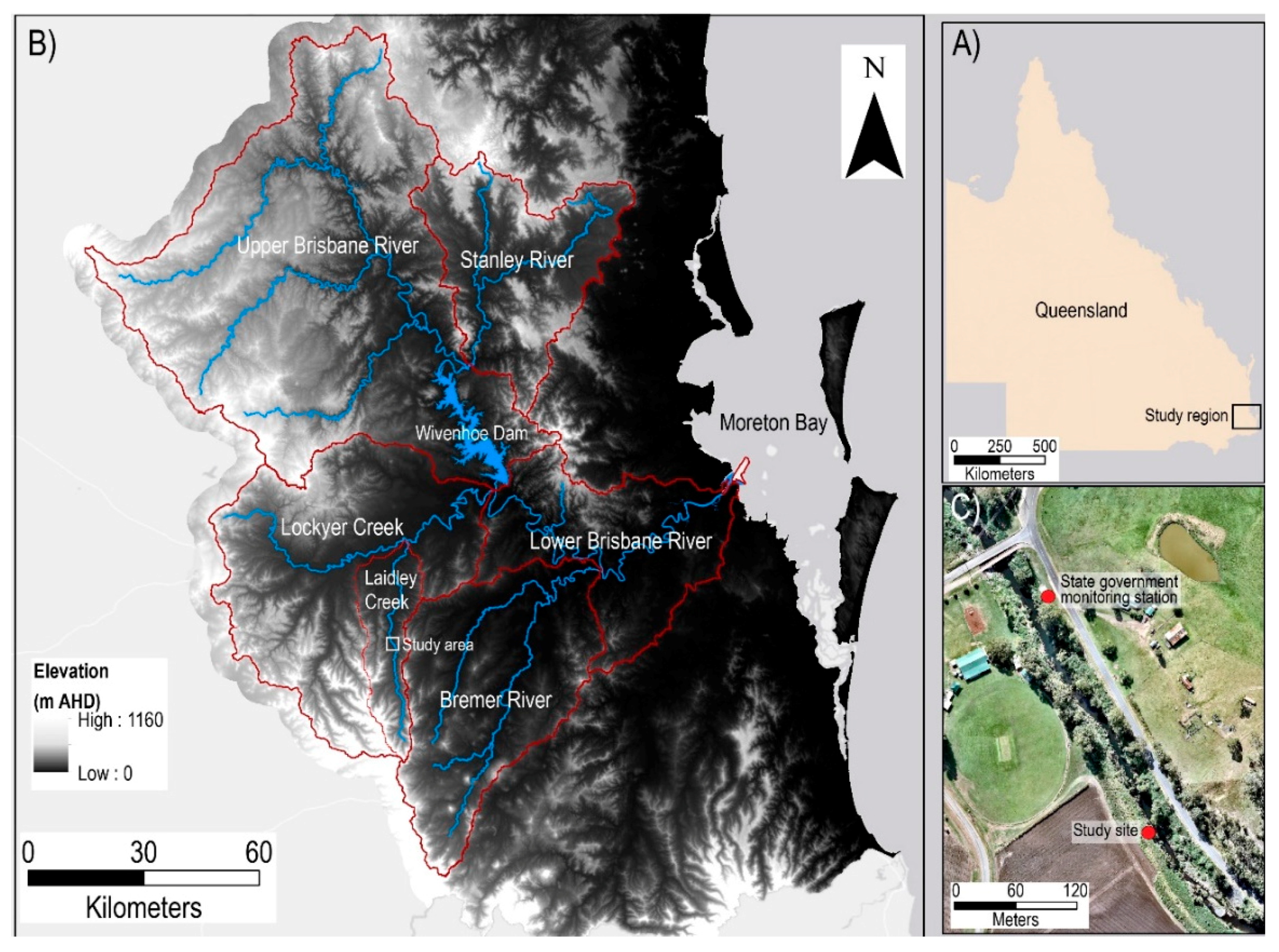
2.1. Study Site Description

Laidley Creek is located in South East Queensland, Australia (Figure 2A), a sub-tropical region prone to large, irregular rainfall events [8]. The creek has a catchment surface area of 462 km2 and runs for approximately 60 km, with much of the course through highly erodible alluvium plains. The original vegetation cover was dominated by dry sclerophyll forest and the riparian vegetation cover is typically mixed eucalypt, casuarina, and wattle forest [9]. However, the catchment is highly modified, with a large-scale clearing of forest trees in the late 1800s resulting in present day landuse dominated by grazing and high intensity agriculture [4]. It is a sub-catchment of the larger Lockyer catchment, and previous studies of both the Laidley Creek and Lockyer Creek systems have clearly demonstrated that the erosion processes are dominated by gulley and channel erosion [10,11]. The creek banks are highly degraded, with limited riparian vegetation remaining and very steep channel profiles. During flood events, large sections of the channel are eroded, resulting in the loss of huge quantities of sediment from the upper catchments. The finer sediment fractions (silts and clays) of this material are transported several hundred kilometers downstream to Moreton Bay [4]. The Lockyer catchment is part of the Brisbane River system, which drains over 13,000 km2 into the coastal embayment, Moreton Bay (Figure 2B). The gulley and channel erosion of the upper catchments has resulted in rapid infilling of the Moreton Bay with terrestrial silts and clays [6,7].
The deployment of a low-cost monitoring network was undertaken upstream of the Beckman Rd Bridge across Laidley Creek at Mulgowie, Queensland, Australia (Figure 2C). Initial aerial surveys of the study sites were undertaken in July 2016, shortly after extensive streambank works were undertaken to rehabilitate the western bank (Figure S1). The long-term streamflow monitoring at Mulgowie gauging station (1967–present) recorded a median of 0.08 m3/s, a mean of 0.83 m3/s, and a maximum of 349 m3/s. These highly variable flow rates indicate that the system is event-driven, with 90% of the annual flow occurring during the summer rainfall period [12]. The low-cost monitoring network was deployed between 29 March 2017 and 1 April 2017 to capture a major flood event resulting from the passage of Ex-Tropical Cyclone Debbie across the study region. On 30 March 2017, over 170 mm of rainfall was recorded in 24 h at Laidley Creek at the Stony Creek Rd monitoring station located 16 km upstream of the study site [13], and the peak water level of 9.35 m was the second-highest on record, just below the maximum of 9.37 m in January 2013 [12].

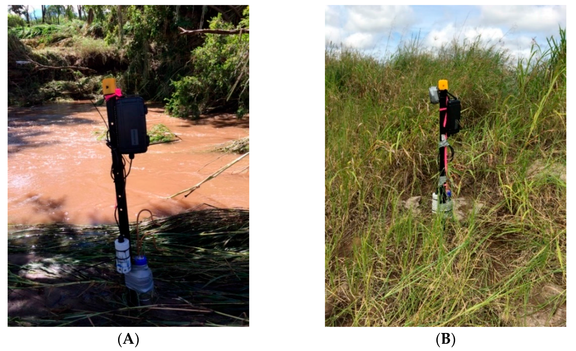
2.2. Field Monitoring

The low-cost monitoring of TSS concentration was undertaken using custom-built sensors as described in Appendix A, and each sensor has a total parts cost under US$150 (Table A1, Appendix A). Raw sensor output was converted directly to TSS concentration following the methodology in (Figure A5) [14]. In addition to the low-cost sensors, single stage samplers were deployed in parallel to collect discrete samples for analysis of suspended sediment particle size distribution and total nutrient concentrations. Time-lapse cameras (Panda UV535 trail camera, UOVision Australia, Oakleigh South, VIC, Australia) were utilized to record changes in water level and colour at 5-min intervals. The total cost of a single monitoring node, consisting of one 1.8 m star picket (US$9), one low-cost sensor (US$148), one single stage sample (US$35), and one time-lapse camera (US$190), was less than US$400.
Monitoring nodes were deployed along an elevation gradient up the streambank to capture changes in sediment loading across different stages of the hydrograph (Figure 3). The deployment configurations were mounted on star pickets driven into the bank and followed the methodology outlined in [3]. A total of seven monitoring nodes were deployed across the site with sensor heights ranging from 0.2 m to 9.5 m above local water level, which were then referenced to the State Government gauging station (Figure 2C). Local stream height changes were recorded using a non-vented underwater pressure transducer (Level TROLL 400 Data Logger, In-situ, Fort Collins, CO, USA), which was deployed immediately adjacent to the lowest monitoring node. The pressure transducer was anchored in a 0.3 m water depth using a star picket and the water level was logged at 1-min intervals for the duration of the deployment. During zero flow conditions, surface and sub-surface (10 cm depth) sediment samples were collected within the creek bed for analysis of particle size distribution. The surface extent of bed material deposits was estimated immediately upstream of the study site by visual inspection of a series of holes dug across the deposit at 5-m intervals.

2.3. Laboratory Analysis

Water samples from single stage samplers were retrieved within 24 h of peak flows. A total nitrogen and total phosphorus analysis was undertaken on these samples using standard methods [15] by the National Association of Testing Authorities, Australia (NATA)-accredited laboratory Environmental Analysis Laboratory at the Southern Cross University. To better understand the relative contribution of washload to downstream nutrient loading, subsamples from two single stage samplers were sieved through a 63 µm sieve to remove the sand fraction and the filtrate was analysed for total phosphorus and total nitrogen.
Samples of suspended and bed material for analysis of particle size distribution were sonicated for one minute prior to measurement to separate aggregated particles, allowing the true particle size to be calculated [16]. Particle sizing was undertaken using laser diffraction (Malvern Mastersizer 2000E, Malvern Instruments Ltd., Malvern, UK), and five measurement cycles were performed for each sample. Sediments were classified according to the Wentworth scale, with mud fractions defined as sediment particles with a diameter of <63 µm [17].
Given the extreme TSS concentrations as well as the obvious sand fractions in the single stage samples collected during high flows, a whole-water test was undertaken to determine how representative the TSS particle size distribution estimated by laser diffraction was. The issue of obtaining representative sub-samples for particle size distribution or TSS concentration from samples with significant sand fractions has been well-established [18]. The whole-water test followed the methodology outlined in [19], where a 12:10 p.m. single stage sample was wet sieved through a 63 µm micron sieve and the sand and mud fractions were dried at 105 °C. The relative sand and mud fractions were determined gravimetrically and expressed as a percentage. TSS concentrations were determined gravimetrically, where samples were filtered using a dried pre-weighed 0.7 µm filter (Whatman glass microfiber filter GF/F grade) and then dried at 105 °C to a constant weight. Filters were reweighed and the TSS concentration (mg/L) was then calculated from the filter weight difference and normalized to the sample volume.

2.4. Imagery Analysis

To obtain high-resolution imagery of the study site before and after a flood event, a series of drone flights were undertaken in July 2016, one day before the flood event (29 March 2017) and one day after the flood event (31 March 2017). The DJI Phantom 3 Pro platform was utilized with the camera (DJI FC300X with a 12 megapixel RGB sensor) in a nadiral orientation for mapping flights. Georeferenced imagery was downloaded from the drone and images selected for photogrammetric data processing. Data processing was undertaken using dedicated processing software (Pix4D Promapper, Pix4D SA, Lausanne, Switzerland), and the resulting mosaics were visualized using the geographical information system ArcGIS (Version 10.3, ESRI Inc., Redlands, CA, USA).

3. Results

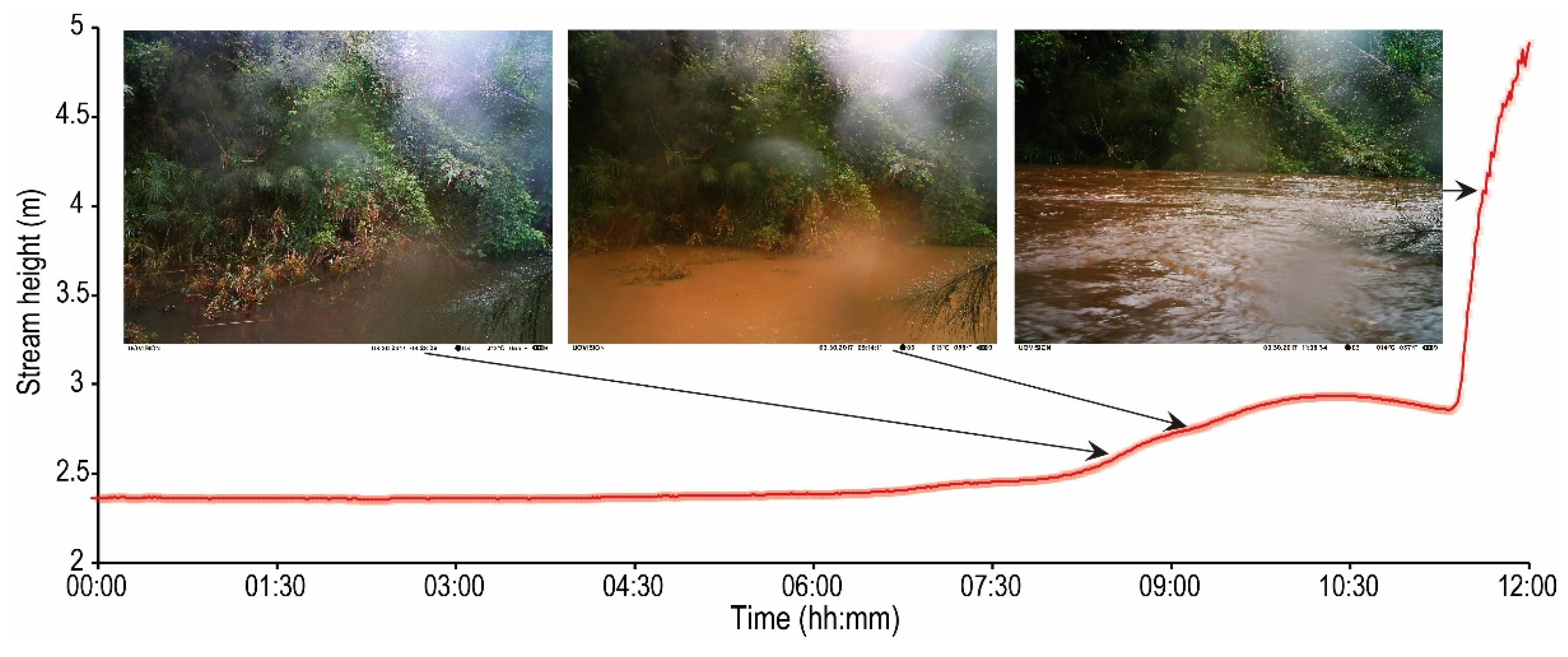
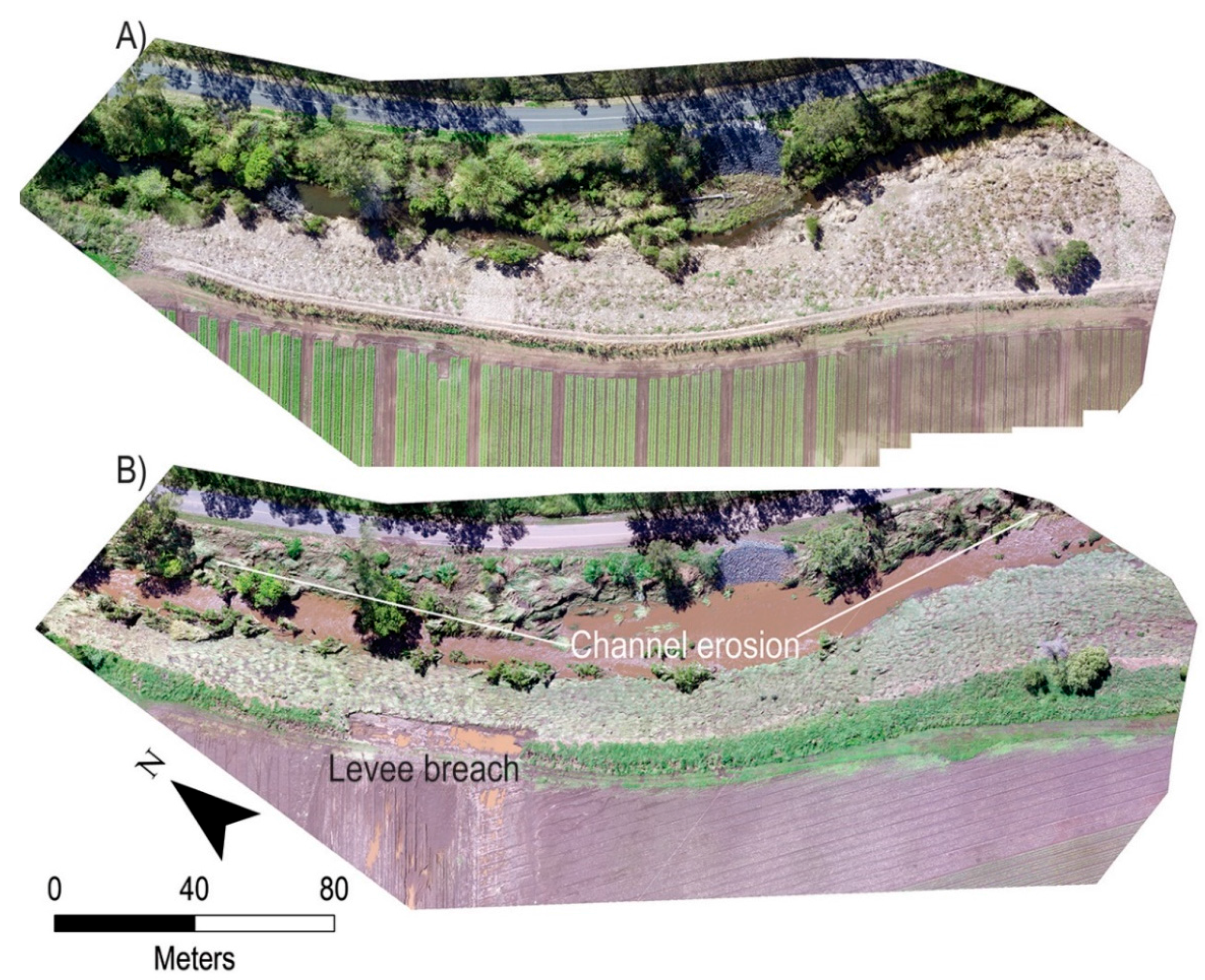
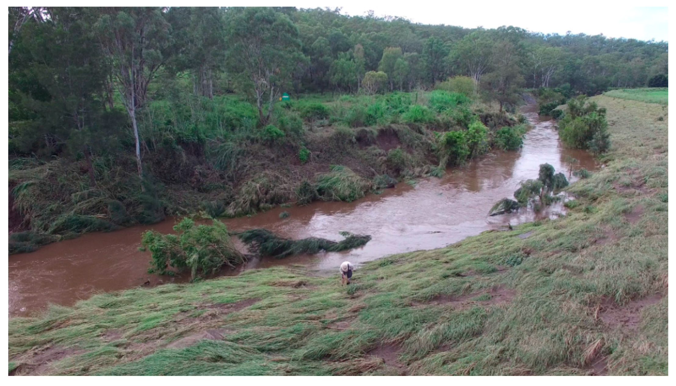
3.1. Time-Lapse and Drone Imagery

High-resolution drone mosaics before and after the event provided a detailed picture of the impact of this flood event, with clear signs of erosion on the natural eastern bank as well as the levee breach on the rehabilitated western bank (Figure 4A,B; Video S1; Video S2). Erosion of the natural bank occurred along at least 250 m of the creek channel upstream from the study site, with slope failures resulting in up to 3 m (horizontal) and 4 m (vertical) of bank loss (Figure 4B; Video S3). The levee breach on the rehabilitated bank highlighted the extreme nature of the flood event, as this was designed to withstand major floods (Figure 4B; Video S4).
Oblique imagery from the site highlighted the contrast between the natural bank and the rehabilitated bank (Figure 5). Despite being on the inside bend, the natural bank experienced substantial erosion, whilst the rehabilitated bank on the outside of the bend was largely stable (Figure 5). This further highlights the potential for streambank rehabilitation to reduce sediment loading from channel erosion, a critical sediment loading source to Moreton Bay [6,11].

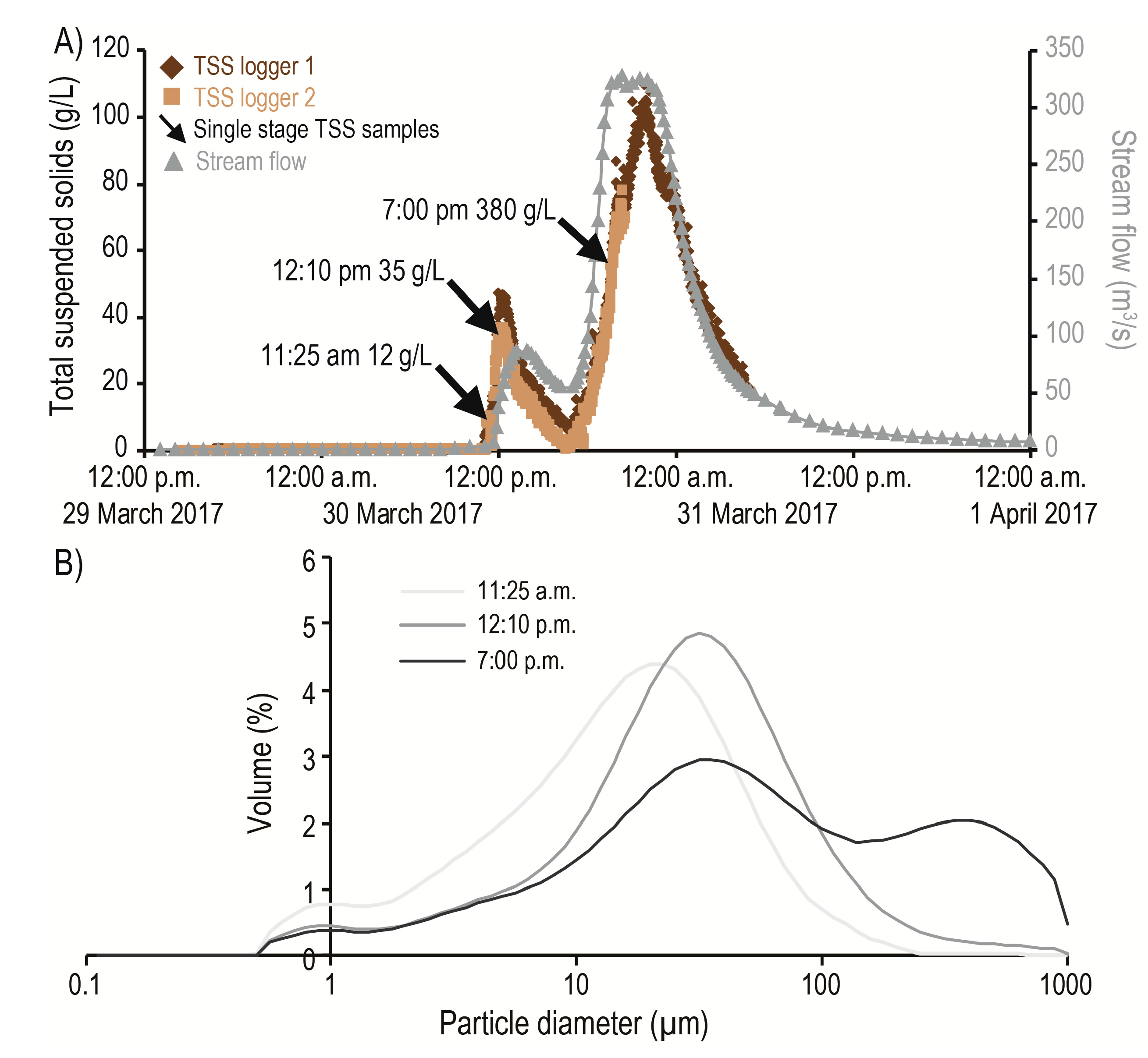
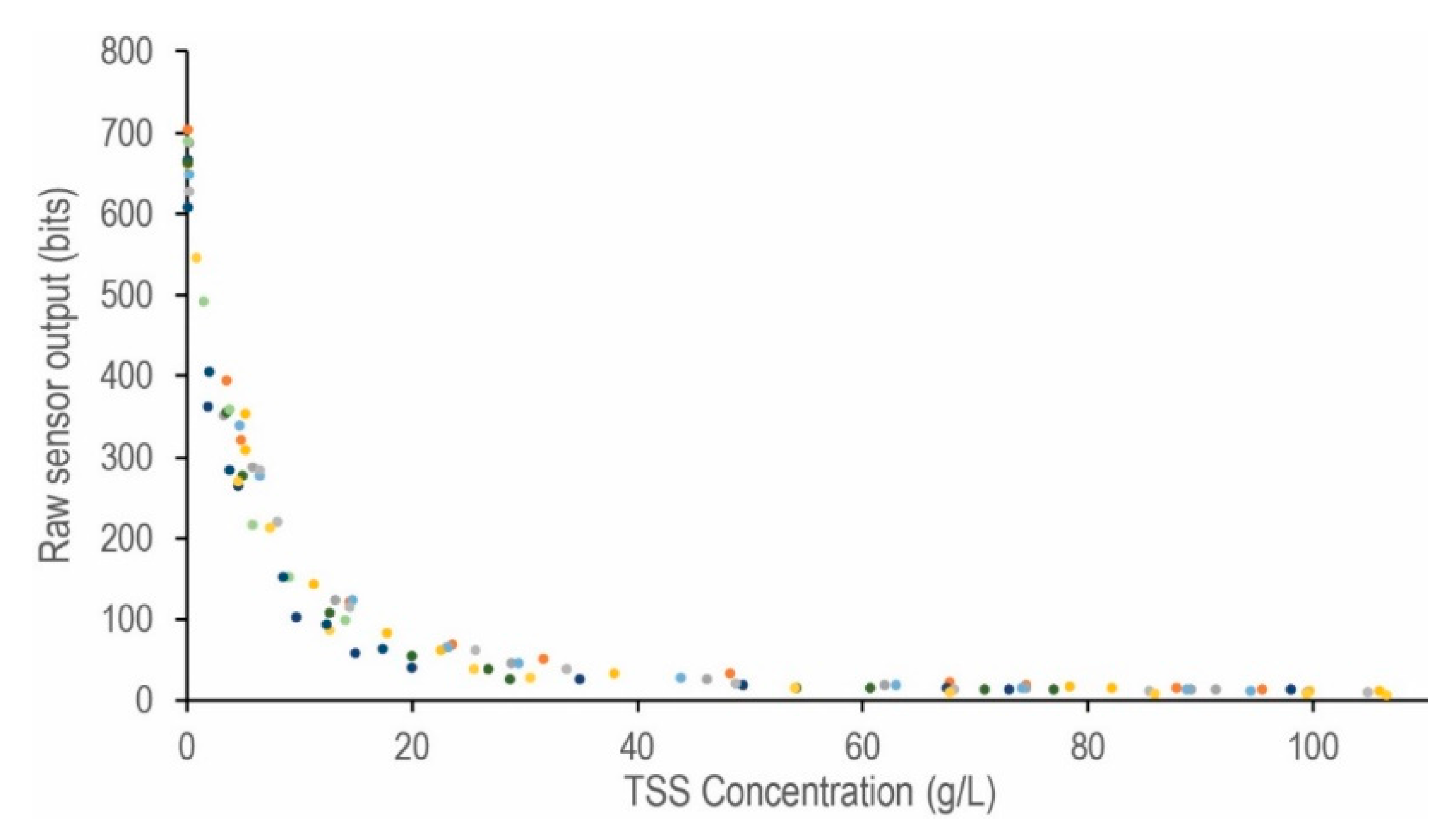
3.2. Suspended Sediment Dynamics

The stream flow across this major flood event consisted of a relatively small initial peak of 86 m3/s occurring at 1:00 p.m. followed by the far larger peak of over 320 m3/s occurring after 8:00 p.m. on 30 March 2017 (Figure 6A). Due to the extremity of the flood event, only two of the seven sensors deployed were recovered (Figure S2). Logged TSS concentrations were strongly correlated to streamflow across the event; however, the timing of peaks in the TSS and streamflow differed slightly. The initial flows were characterised by a peak in the TSS that preceded the peak flow; this was followed by a lag in the TSS peak with the much higher secondary peak in streamflow (Figure 6A). Changes in TSS concentrations were mirrored by both loggers recovered, although logger 2 lost its sensor just prior to the major peak flow. The majority of suspended sediment transport occurred at high flow rates, with TSS concentrations recorded above 80 g/L by both TSS loggers as well as by a single stage sampler. A large discrepancy was observed between the TSS concentration of the 7 p.m. single stage sample (384 mg/L) and that of the logged values (57 and 59 mg/L) recorded at this time (Figure 6A). Overall, these data are in contrast to the long-term event monitoring undertaken by the State Government, where event mean concentrations from 203 samples collected between 2002 and 2015 averaged 0.272 g/L and ranged between 0.094 and 0.762 g/L [20,21]. Whilst these data include a number of small flow events, there were at least two major floods (in 2011 and 2013) that occurred in this time period and that recorded similar peaks to this 2017 event.
The suspended sediment particle size distribution across the event clearly showed an increasing contribution from sand particles during higher flows (Figure 6B). Relatively low flows were almost exclusively composed of fine silt and clay sediment particles (D10% 2.3 µm; D50% 14.8 µm; D90% 50.4 µm). The increasing contribution from sandy particles is observed in the D90% particle diameter, which increased from 50.4 µm (coarse silt) at 11:25 a.m. to 92.5 µm (very fine sand) at 12:10 p.m. and 448 µm at 7:00 p.m. (medium sand). Particle sizing using laser diffraction heavily favoured the fine particles. At 12:10 p.m., the mud fraction was estimated to be 80%; however, the sieve analysis of the whole sample estimated the mud fraction to be 40%. This is likely due to the difficulty associated with taking a truly representative sample for laser diffraction with slurries containing such a high sand fraction. The issue of obtaining representative sub-samples applied to quantifying TSS concentrations in the single stage as well, with sub-samples approximately 10% lower than whole-sample estimates.

3.3. First Flush Phenomenon

The first flush is often defined as the disproportionate increase in concentration of soluble and particulate materials during the rising stage of a flow event [21]. The initial flows observed in this study underwent a first flush phenomenon, as water colour rapidly changed from transparent to highly coloured with a very small rise (approximately 20 cm) in water level (Figure 7; Video S4). The cause of this rapid colour change was a large increase in suspended clay and silt particles (Figure 6B). The water discoloration persisted with the subsequent flows across the whole event (Video S5). Together with the rapid increase in TSS preceding the initial peak (Figure 6A), these data suggest the importance of this ‘first flush’ phenomenon and that even low streamflow events may be important contributors to downstream sediment loading.
A large sandy deposit was observed within the creek channel immediately upstream of the study site with a surface area of approximately 174 m2 and a minimum deposit depth of 70 cm (Figure 8A). The entire surface of this deposit was covered in a thin crust between 1 and 3 cm deep, which was greatly enriched in silt and clay fractions (50% mud) relative to the underlying sandy bed material (10% mud) (Figure 8B).
Total nutrient concentrations were highly elevated in both the single stage samples collected at relatively low flows and relatively high flows (Table 1). In addition, there was relatively little change between total nutrient concentrations of total and sieved samples, which suggests that much of the nitrogen and phosphorus species was associated with the washload (Table 1). The association of phosphorus with fine sediment particles in washload has been observed during high flow events in this region [22]. Total nitrogen concentrations during the high flows at 7:00 p.m. were lower concentrations after sieving (Table 1). In this region, total nitrogen is dominated by the particulate organic nitrogen fractions during high flows [23], and larger fragments may have been trapped by the sample sieving, reducing the concentration of total nitrogen. Long-term event monitoring total nutrient concentrations from the State Government event station were approximately one order of magnitude lower than those found in the single stage samples (Table 1).

4. Discussion

This study successfully captured changes in near-bed TSS concentrations across a major flood event using a low-cost approach. Changes in suspended sediment particle size distribution clearly showed the increasing contribution of sandy fractions to TSS as the flood event developed. Total nitrogen and phosphorus fractions were closely associated with washload, suggesting that the majority of nutrient load was exported from this system to downstream receiving water bodies. The near-bed TSS concentrations were in excess of that required to hinder settling (5 to 10 g/L) of suspended sand particles [24]; this would reduce the settling rates of these particles and, therefore, increase their time in suspension and subsequent transport distances downstream [25].
We suggest that the first flush phenomenon observed in this study is a result of local resuspension of muddy crusts immediately upstream of the monitoring site. Whilst this resulted in relatively high TSS concentrations in the near-bed, the higher flows experienced subsequently entrained the underlying sandy bed, which resulted in the extreme TSS concentrations during peak flows. The widespread channel erosion occurring throughout the creek system would likely result in a continuous sediment supply across the event. The finer mud fractions would settle more slowly than the sandy particles as the flood event recedes, reforming the muddy crusts observed in the stream bed. This behavior has been clearly demonstrated in laboratory experiments examining sand-mud suspensions [26].
The discrepancy in TSS concentration between the 7 p.m. single stage sample and the logged values was likely due to the shroud structure surrounding the low-cost sensors (Figure A1). This shroud would shield the sensor face from direct water flows, slowing the near-field water velocities and allowing larger sand particles to rapidly settle in this zone [27]. The net effect would reduce the concentration of sand particles passing the sensor face and greatly reduce the observed TSS concentrations [28]. The lower flows during the initial stage of the flood event were dominated by silt and clay fractions which would not settle as quickly and showed good agreement between single stage measurements and logged values. In addition, the extremely high TSS concentrations during peak flows resulted in the sensors approaching their upper detection limits (Figure A5) [14]. These limitations will form the basis of future research to improve the shroud design and sensor signal-to-noise ratio at extreme TSS concentrations.
The TSS and total nutrient concentrations observed in this study were greatly elevated compared to the long-term monitoring data from the State Government event station located approximately 250 m downstream. The pump inlet for the event station was located on the stream bed and would have been exposed to similarly high concentrations of suspended bed material and washload as the low-cost sensors. One explanation for this discrepancy lies in the protective cover surrounding the pump inlet (Figure 1C) as well as the 500-μm screen on the inlet pipe. This would greatly reduce water flow in the immediate vicinity of the inlet as well as physically filter out much of the coarser fraction of the suspended bed material prior to collection. Sediment particle fractions that were able to pass through these would likely be limited to very fine particles, which would lead to significant undersampling of the actual sediment load [27]. This highlights an area of uncertainty in current event-monitoring practices; standardisation of the inlet structure and its elevation above the bed should be considered in standard operating procedures in order to ensure comparable results are obtained. For instance, sample collection systems that integrate over the entire water column as described in [29] should be considered.
These findings have direct relevance to understanding and analysing sediment budgets, e.g., the contribution of catchment-wide sediment yield, erosion from upstream channel regions or floodplain sources, and changes to the volume and residence time within the system [30]. Particularly in larger catchment areas, the quantification of these processes is complex [31]. Careful and extensive monitoring is required [32,33], which poses a logistical and financial challenge in many river systems from mountainous streams to the ocean. In addition, the variation of suspended sediment concentration during flood events as reported here and in numerous other studies [34,35,36,37,38,39] adds to the difficulty and uncertainty of an efficient and robust monitoring strategy.
The development of a truly low-cost approach to monitoring sediment dynamics during flood events will provide an opportunity for spatially intense regional monitoring programs as well as a cost-effective method to quantify vertical TSS gradients at single sites. This is of particular importance to guide catchment rehabilitation management actions where it will be critical to separate the effects of regional landuse changes from local stream bed effects. In addition, as climate-induced changes in rainfall patterns increase the likelihood of extreme flood events [40], this low-cost approach will provide an important addition to the existing monitoring of these events. The simplicity of the approach will also provide opportunities globally to deploy these sensors in areas currently lacking any formal monitoring system.

Supplementary Materials

The following are available online at https://www.mdpi.com/2073-4441/10/2/34/s1, Figure S1: Drone images facing upstream from study site showing: (A) Recently completed earth works on rehabilitated left hand bank in July 2016; and (B) successful revegetation of rehabilitated bank one day prior to flood event in March 2017. Figure S2. (A) High resolution drone mosaic of study site immediately after the major flood event, showing the recovery status of deployed nodes at the study site and the upstream site. Image collected on 31 March 2017. (B) Creek cross-section transect prior to flow event from study site and the relative position of deployed nodes. Note that two nodes were placed at the lowest position. (C) Zoomed image of a tree trunk deposited during peak flows; the trunk was 9 m long and 1.3 m in diameter. Video S1: One_Day_Before_Flood, Video S2: One_Day_After_Flood, Video S3: Channel_Erosion, Video S4: Mulgowie_High_Camera_9_m, Video S5: Mulgowie_Low_2_m, Computer code folder 1: S1_Sensor_Code, Computer code folder 2: S2_Sensor_Code.

Acknowledgments

We acknowledge The University of Queensland and Port of Brisbane Pty Ltd. Research Partnership for providing financial support to this study. Graham Lancaster from the EAL, Southern Cross University is gratefully acknowledged for advice on appropriate analysis techniques.

Author Contributions

P.F., A.G., and N.D. conceived and designed the low-cost sensors; all authors contributed to study design and data analysis; S.A., N.D., and A.G. undertook field deployments; M.L. contributed background information and facilitated access; A.G., N.D., S.A., and R.C. wrote the paper.

Conflicts of Interest

The authors declare no conflict of interest.

Appendix A

To develop a regional monitoring network of fluvial suspended sediment discharge during high flow events, a low-cost sensing solution was required. The low-cost system is manufactured from a commercial washing machine turbidity sensor (TSD-10 Turbidity Sensor, Amphenol Advanced Sensors, Wallingford, CT, USA) calibrated to total suspended sediment concentration. The sensor system is assembled in three parts: the electronics board, the housing and battery assembly, and the sensor assembly (Figure A1). The total cost of the parts, outlined in Table A1, is US$147.66.
Figure A1. Example of a completed low-cost sensor and housing layout.
Water 10 00034 g0a1

Appendix A.1. Sensor Assembly

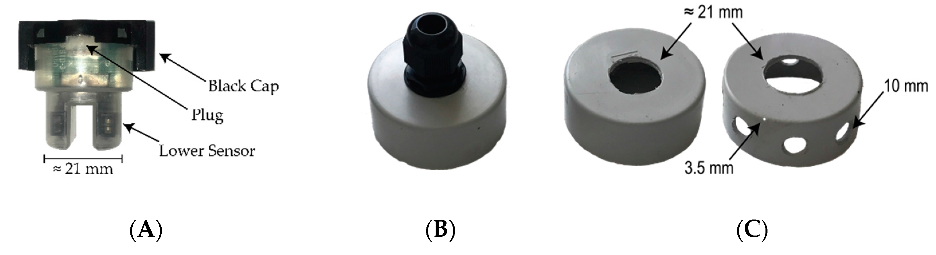
  • Drill a 21 mm hole in the top of two 50 mm PVC caps (Figure A2C) corresponding to the diameter of the lower section of the Amphenol Sensor (Figure A2A). Then, drill eight (10 mm) holes evenly spaced around the cap flange and four holes (3.5 mm) in the inner edges of one cap, cleaning all burrs. Ensure both caps are clean and glue the two caps back to back with PVC cement/glue.
    Figure A2. (A) Amphenol sensor. (B) Third PVC cap and cable gland. (C) Two caps produced in step 1 for forming the bottom of the sensor assembly.
    Figure A2. (A) Amphenol sensor. (B) Third PVC cap and cable gland. (C) Two caps produced in step 1 for forming the bottom of the sensor assembly.
    Water 10 00034 g0a2
  • Measure the diameter of the waterproof cable glands threaded section (≈19 mm) and drill the corresponding size hole in the centre of the third 50 mm PVC Cap. Clean the edges of the hole, ensuring there is no burr or raised markings. Secure the cable gland in the drilled hole (Figure A2B). Hot glue can be used on the nut of the gland to provide additional support when tightening.
  • Cut a 75 mm length of 50 mm diameter PVC pipe, clean the edges of the cut.
  • Cut the appropriate length of cable for the proposed deployment, noting that the length should be 500 mm greater than required.
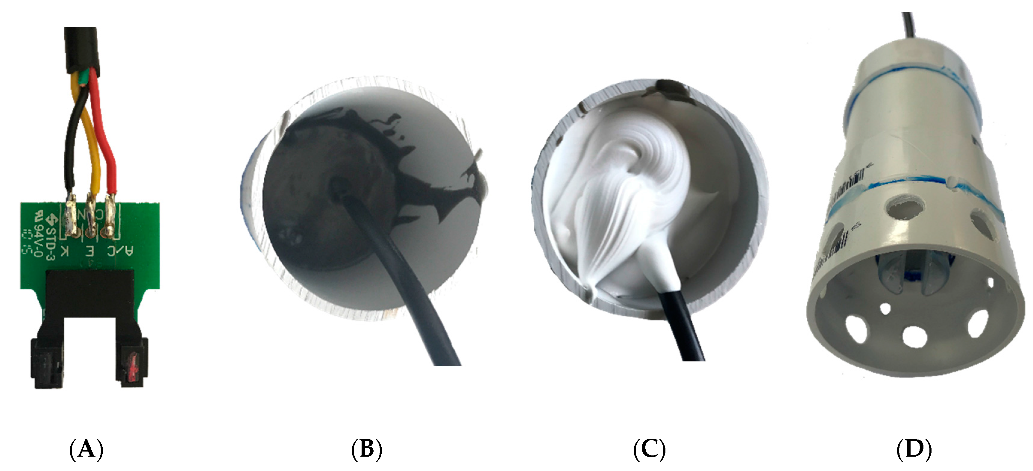
  • Strip 50 mm of outer black coating from both ends of the sensor cable. Then, strip a small amount (≈10 mm) from the red, yellow, and internal black wire covers. Cut the green cable off to the same level at the outer black coating (Figure A3A).
  • Twist the ends of the exposed wires separately and apply lead-free solder.
  • Remove the black cap from the Amphenol Sensor and then remove the sensor board from the clear housing. Cut the white plastic plug off the sensor board, and then solder the sensor cable wires to the uncovered pins (Figure A3A), covering connections in heat-shrink or electrical tape. Place the sensor board back into the housing and reattach the black cap, ensuring that the sensor cable exits through the hole. Seal the cable gap with hot glue.
    Figure A3. (A) Illustrating the cable soldered on the sensor board, ensuring the solder does not bridge between the sensors. The wires connected as; Red to A/C, Black to K, and Yellow to E. (B) Epoxy-filled sensor housing. The harder epoxy is first to provide a dense base, and hold the cable firmly in place to prevent movement of the soldered joint. (C) Silicon filling is used in the top to provide a more flexible housing fill so the cable can be positioned for the top cap. (D) Completed sensor assembly.
    Figure A3. (A) Illustrating the cable soldered on the sensor board, ensuring the solder does not bridge between the sensors. The wires connected as; Red to A/C, Black to K, and Yellow to E. (B) Epoxy-filled sensor housing. The harder epoxy is first to provide a dense base, and hold the cable firmly in place to prevent movement of the soldered joint. (C) Silicon filling is used in the top to provide a more flexible housing fill so the cable can be positioned for the top cap. (D) Completed sensor assembly.
    Water 10 00034 g0a3
  • Place the sensor into the glued caps assembled in Step 1, ensuring that the lower section of the sensor is the on the side of shroud. Hot glue the sensor in this position, and slide the pipe down the cable. Glue the lower caps and the pipe together with PVC cement/glue (Figure A3D).
  • Position so the opening in the pipe is facing up, and prepare the Araldite epoxy as per the manufacturer’s instructions. Pour epoxy into the pipe until 10–20 mm above the black cap, and agitate to remove the air voids while topping up with epoxy as required. Sit for 24–48 h until epoxy is fully set (Figure A3B).
  • Fill the remaining void area with waterproof silicon (Figure A3C), and then pull the sensor cable through the cable gland. Use PVC cement/glue to affix the top cap to the pipe, and then tighten the gland around the cable to seal the assembly.

Appendix A.2. Case and Power Supply Assembly

11.
Drill a hole corresponding to the diameter of the cable gland threaded section in the acrylonitrile butadiene styrene (ABS) case on the opposite side to the attachment strap. Clean burrs and remove the inner foam lining around the hole. Affix the second cable gland in the hole using hot glue to prevent excessive spinning of the nut.
12.
Collect the battery holder and solder the red jumper wire to the red battery holder wire and the black jumper wire to the black battery holder wire. Cover the joints in heat-shrink or electrical tape.
13.
Place batteries in the holder and test the voltage (7.2 V).

Appendix A.3. Electronics Board Assembly

14.
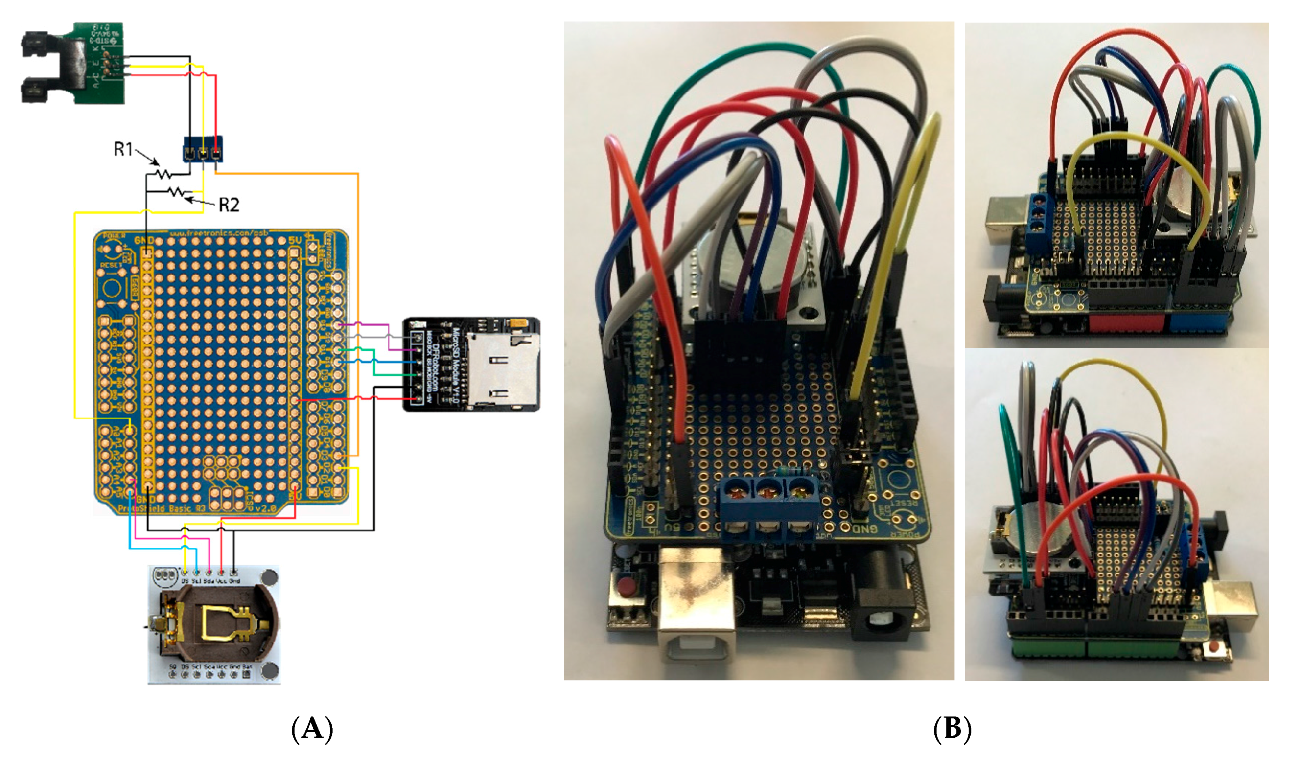
Solder the stacking header to the outer holes in the prototyping board, and ensure that this can bridge to a DRFudino board (Figure A4B).
15.
Once the stacking headers are in place, the inner headers are soldered in an upright orientation; this allows for easy wiring of the circuit.
16.
Finally, the electronic components are added following the wiring pattern in Figure A4A.
Figure A4. (A) Electronics wiring schematic for the electronics board applicable for the code provided. For the Amphenol TSD-10 sensor used, the R1 resistor is 4700 Ohms and R2 is 470 Ohms. (B) Preassembled board and recommended configuration.
Water 10 00034 g0a4

Appendix A.4. Final Assembly

17.
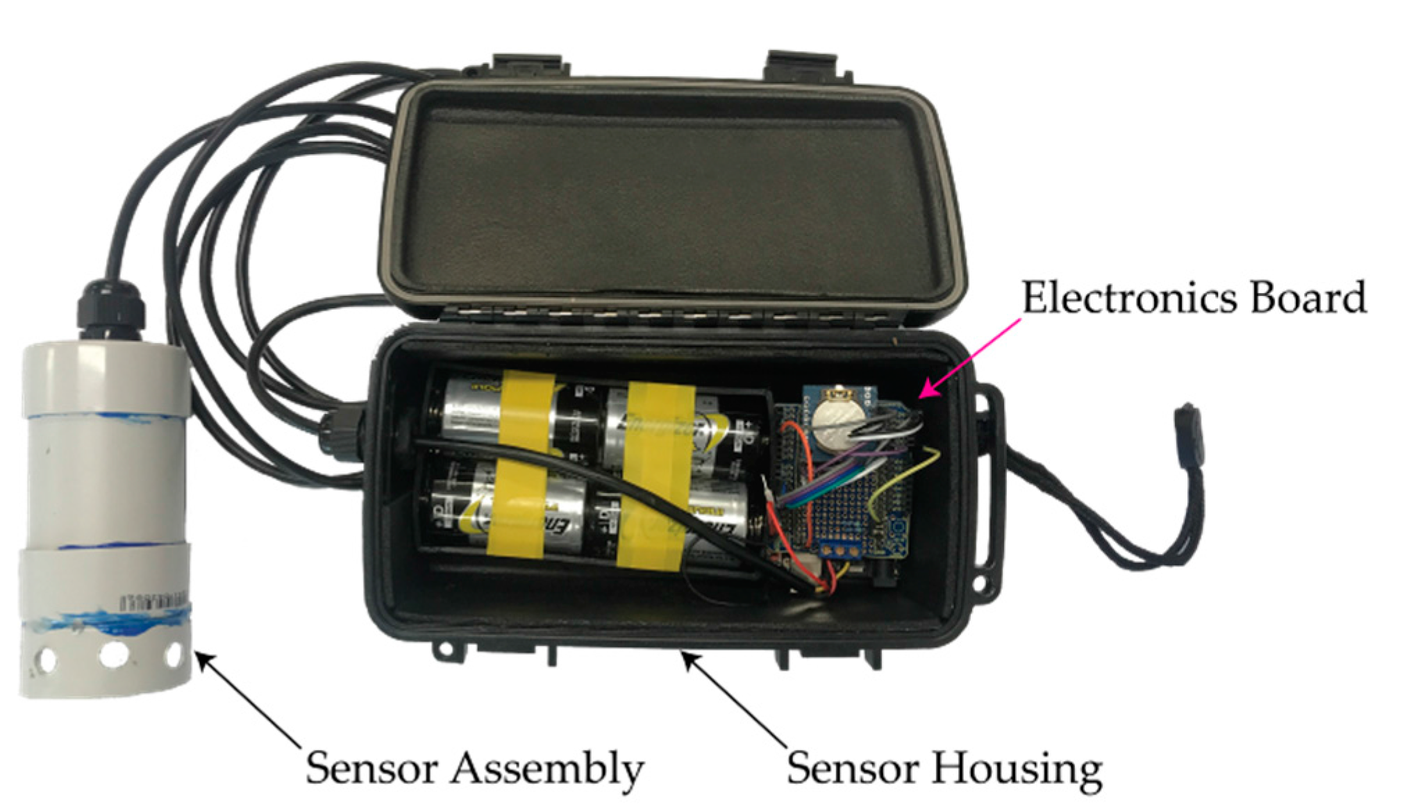
Place components in the ABS housing case (Figure A1).
18.
Connect the battery to the electronics board by plugging the red wire from the battery pack to Vin and the black wire to ground pin (GND). Ensure the red light on the electronics board lights up, then remove the battery wires until deployment.
19.
Run the sensor cable through the cable gland in the housing and connect the wires as shown (Figure A4A). Before tightening the gland around the cable, ensure that there is extra cable length for board movement within the case.

Appendix A.5. Programing

20.
Download the Arduino program from the Arduino website.
21.
Install the relevant libraries, outlined in Code S1.
22.
Connect the electronics board to the computer.
23.
Set the real-time clocks using the corresponding code (Code S2).
24.
Upload the sensor code to the board (Code S1). Note that the monitoring frequency can be adjusted within the code, the default is 10 s of monitoring.
25.
Check that the code is running, the time is correct, and the sensor functions correctly (bits reduce when the sensor is blocked) by opening the serial monitoring portal.

Appendix A.6. Deployment

26.
Connect the battery pack to the electronics board (Red: Vin, Black: Ground)
27.
To check that the sensor is functioning correctly, log 3–5 monitoring intervals. Disconnect the battery, remove the storage device (SD) card, and check readings. If functioning correctly, reinsert the SD card and then reattach the battery.

Appendix A.7. Calibration

Low-cost sensor laboratory calibration was undertaken using a silica-based slurry at increasing concentration across the sensor measurement range (200 mg/L to 120 g/L). After each increase in TSS concentration, the sensor signal was monitored until this stabilised, usually after a period of one minute, until no further change in signal was detected. The concentrations observed during the higher flow stages mean that the sensor itself was likely to be at or above its detection limit. The sensor appears to have a reasonable signal-to-noise ratio at concentrations below 30 g/L; however, the peak concentrations recorded were well above this threshold (Figure A5). The single stage TSS estimates at lower flow rates agreed well with the logged data; however, at high flows the single stage TSS concentration was almost 5 times higher compared with the logged values. Future research will trial higher-range sensors to better quantify the loads during high flows.
Figure A5. Sensor signal-to-noise ratio from increasing suspended sediment concentrations under controlled laboratory conditions [14].
Water 10 00034 g0a5

Appendix A.8. Required Parts

Table A1. A complete list of required parts, consumables, and tools required for the assembly of a low-cost sensor, prices as of November 2017.
QtySupplierPart #Cost (US$)
Electronics Board
DFRduino UNO R3—Arduino Compatible1DFRobotDFR0216$15.19
MicroSD card module for Arduino1DFRobotDFR0229$3.97
Real Time Clock Module (DS1307) V1.11DFRobotDFR0151$3.36
10 Pcs 40 pin Headers Straight1DFRobotFIT0084$2.37
4.7 k Ohm 0.5 Watt Metal Film Resistor1JaycarRR0588$0.42
470 Ohm 0.5 Watt Metal Film Resistor1JaycarRR0564$0.42
2 GB Class 4 microSD Card1JaycarXC4998$7.60
3 Way PCB Mount Screw Terminal—5 mm Pitch1JaycarHM3173$1.18
ProtoShield Basic for Arduino1FreetronicsPSB$2.29
Shield stacking headers for arduino (R3 compatible)1Adafruit85$1.49
Sub-total$38.28
Sensor Assembly
Amphenol Advanced Sensors TSD-101Mouser ElectronicsTSD-10$8.24
50 mm PVC DWV Pipe1 mBunnings4770087$5.40
50 mm PVC Caps3Bunnings4750164$6.30
Multipurpose Water Proof Silicon1Bunnings1232705$4.08
5–10 mm DIA IP68 Waterproof Cable Glands—Pk.21JaycarHP0727$4.54
Sealer Araldite Epoxy K1061Blackwoods00405455$22.14
14/0.20 Black 4 Core Security Cable5 mAltronicsW2355$8.40
Sub-total$59.11
Housing and Power Supply
Case Abs Blk IPX8 210 × 120 × 90 mm1JaycarHB6425$26.68
4 × D CELL 2 Rows of 2 battery holder1JaycarPH9222$2.25
D cell Alkaline Batteries4 $6.07
Sub-total$35.00
Consumables
Hot glue
Lead free solder
PVC cement for pressurised pipes
Jumper shunts (links)2JaycarHM3240
Premium Female/Male ‘Extension’ Jumper Wires—40 × 3′′ (75 mm)1Adafruit825
Premium Female/Female Jumper Wires—40 × 3′′ (75 mm)1Adafruit794
Heat-shrink or electrical tape
Sub-total$15.27
Total$147.66
Required Tools
Soldering iron
Hack saw
Drill
Drill bit (3.5 mm, 10 mm, 19 mm, and 21 mm)
Wire strippers and cutters
Phillips head screw driver #1, 2.5 mm shaft
Snap-off or retracting knife (9 or 18 mm)
Measurement tools (Ruler, Calipers)
Multimeter

References

  1. Pelletier, J.D. A spatially distributed model for the long-term suspended sediment discharge and delivery ratio of drainage basins. J. Geophys. Res. Earth Surf. 2012, 117. [Google Scholar] [CrossRef]
  2. Galy, V.; Peucker-Ehrenbrink, B.; Eglinton, T. Global carbon export from the terrestrial biosphere controlled by erosion. Nature 2015, 521, 204–207. [Google Scholar] [CrossRef] [PubMed]
  3. Shellberg, J.G.; Brooks, A.P.; Rose, C.W. Sediment production and yield from an alluvial gully in northern Queensland, Australia. Earth Surf. Process. Landf. 2013, 38, 1765–1778. [Google Scholar] [CrossRef]
  4. Wallbrink, P.J. Quantifying the erosion processes and land-uses which dominate fine sediment supply to Moreton Bay, Southeast Queensland, Australia. J. Environ. Radioact. 2004, 76, 67–80. [Google Scholar] [CrossRef] [PubMed]
  5. Olley, J.; Burton, J.; Smolders, K.; Pantus, F.; Pietsch, T. The application of fallout radionuclides to determine the dominant erosion process in water supply catchments of subtropical South-east Queensland, Australia. Hydrol. Process. 2013, 27, 885–895. [Google Scholar] [CrossRef]
  6. Coates-Marnane, J.; Olley, J.; Burton, J.; Sharma, A. Catchment clearing accelerates the infilling of a shallow subtropical bay in east coast Australia. Estuar. Coast. Shelf Sci. 2016, 174, 27–40. [Google Scholar] [CrossRef]
  7. Lockington, J.R.; Albert, S.; Fisher, P.L.; Gibbes, B.R.; Maxwell, P.S.; Grinham, A.R. Dramatic increase in mud distribution across a large sub-tropical embayment, Moreton Bay, Australia. Mar. Pollut. Bull. 2016, 116, 491–497. [Google Scholar] [CrossRef] [PubMed]
  8. Grinham, A.; Gibbes, B.; Gale, D.; Watkinson, A.; Bartkow, M. Extreme rainfall and drinking water quality: A regional perspective. In Water Pollution XI; Brebbia, C.A., Ed.; WIT: Southampton, UK, 2012; Volume 164, pp. 183–194. [Google Scholar]
  9. Hubble, T.; Docker, B.; Rutherfurd, I. The role of riparian trees in maintaining riverbank stability: A review of Australian experience and practice. Ecol. Eng. 2010, 36, 292–304. [Google Scholar] [CrossRef]
  10. Olley, J.; Wilkinson, S.; Caitcheon, G.; Read, A. Protecting Moreton Bay: How can we reduce sediment and nutrient loads by 50%. In Proceedings of the 9th International River Symposium, Brisbane, Australia, 4–7 September 2006; Volume 47, p. 19. [Google Scholar]
  11. Kemp, J.; Olley, J.M.; Ellison, T.; McMahon, J. River response to european settlement in the subtropical Brisbane River, Australia. Anthropocene 2015, 11, 48–60. [Google Scholar] [CrossRef]
  12. Department of Natural Resource Management. Water Monitoring Information Portal. Available online: https://watermonitoring.information.qld.gov.au (accessed on 25 April 2017).
  13. Australian Government Bureau of Meteorology (BOM). Queensland Rainfall and River Height Data, Stony Creek rd Gauge. Available online: http://www.bom.gov.au/qld/flood/rain_river.shtml (accessed on 2 April 2017).
  14. Gian, J. Improving the Testing of Sedimentation Processes—Development of a Large Column Test and Observations of Solid Concentration Using Turbidity Measurements. Bachelor’s Thesis, The Unversity of Queensland, Brisbane, Australia, 2016. [Google Scholar]
  15. American Public Health Association; American Water Works Association; Water Pollution Federation. Standard Methods for the Examination of Water and Wastewater, 22nd ed.; American Public Health Association: Washinton, DC, USA, 2012. [Google Scholar]
  16. Sperazza, M.; Moore, J.; Hendrix, M. High-resolution particle size analysis of naturally occurring very fine-grained sediment through laser diffractometry. J. Sediment. Res. 2004, 74, 736–743. [Google Scholar] [CrossRef]
  17. Folk, R.L. Petrology of Sedimentary Rocks; Hemphill Pub. Co.: Austin, TX, USA, 1974. [Google Scholar]
  18. Horowitz, A.J. A review of selected inorganic surface water quality-monitoring practices: Are we really measuring what we think, and if so, are we doing it right? Environ. Sci. Technol. 2013, 47, 2471–2486. [Google Scholar] [CrossRef] [PubMed]
  19. Gray, J.R.; Glysson, G.D.; Turcios, L.M.; Schwarz, G.E. Comparability of suspended-sediment concentration and total suspended solids data. In US Geological Survey Water-Resources Investigations Report 00-4191; U.S. Geological Survey: Reston, VA, USA, 2000. [Google Scholar]
  20. Orr, D.N.; Turner, R.D.R.; Thomson, B.; Ferguson, B.; Newham, M.; Wallace, R.; Huggins, R.; Severino, Z. South East Queensland Water Quality Statistics for Event Flow and Base Flow Conditions: 2002–2015; Department of Science, Information Technology and Innovation.: Brisbane, Australia, 2017. [Google Scholar]
  21. Obermann, M.; Rosenwinkel, K.-H.; Tournoud, M.-G. Investigation of first flushes in a medium-sized mediterranean catchment. J. Hydrol. 2009, 373, 405–415. [Google Scholar] [CrossRef]
  22. Kerr, J.G.; Burford, M.; Olley, J.; Udy, J. Phosphorus sorption in soils and sediments: Implications for phosphate supply to a subtropical river in Southeast Queensland, Australia. Biogeochemistry 2011, 102, 73–85. [Google Scholar] [CrossRef]
  23. Garzon-Garcia, A.; Olley, J.M.; Bunn, S.E. Controls on carbon and nitrogen export in an eroding catchment of South-eastern Queensland, Australia. Hydrol. Process. 2015, 29, 739–751. [Google Scholar] [CrossRef]
  24. Dankers, P.J.T. On the Hindered Settling of Suspensions of Mud and Mud-Sand Mixtures. Ph.D. Thesis, Delft University of Technology, Delft, The Netherlands, 2006. [Google Scholar]
  25. Rijn, L.C.V. Principles of Sedimentation and Erosion Engineering in Rivers, Estuaries and Coastal Seas Leo C. van Rijn; Aqua Publications: Amsterdam, The Netherlands, 2005. [Google Scholar]
  26. Amy, L.A.; Talling, P.J.; Edmonds, V.O.; Sumner, E.J.; Lesueur, A. An experimental investigation of sand–mud suspension settling behaviour: Implications for bimodal mud contents of submarine flow deposits. Sedimentology 2006, 53, 1411–1434. [Google Scholar] [CrossRef]
  27. Gettel, M.; Gulliver, J.S.; Kayhanian, M.; DeGroot, G.; Brand, J.; Mohseni, O.; Erickson, A.J. Improving suspended sediment measurements by automatic samplers. J. Environ. Monit. 2011, 13, 2703–2709. [Google Scholar] [CrossRef] [PubMed]
  28. Devlin, M.; Waterhouse, J.; Brodie, J. Community and connectivity: Summary of a community based monitoring program set up to assess the movement of nutrients and sediments into the Great Barrier Reef during high flow events. Water Sci. Technol. 2001, 43, 121–131. [Google Scholar] [PubMed]
  29. Selbig, W.R. Characterizing the distribution of particles in urban stormwater: Advancements through improved sampling technology. Urban Water J. 2015, 12, 111–119. [Google Scholar] [CrossRef]
  30. Trimble, S.W. A sediment budget for Coon Creek basin in the driftless area, Wisconsin, 1853–1977. Am. J. Sci. 1983, 283, 454–474. [Google Scholar] [CrossRef]
  31. Wallbrink, P.J.; Murray, A.S.; Olley, J.M.; Olive, L.J. Determining sources and transit times of suspended sediment in the Murrumbidgee River, New South Wales, Australia, using fallout 137Cs and 210Pb. Water Resour. Res. 1998, 34, 879–887. [Google Scholar] [CrossRef]
  32. Dietrich, W.E. Settling velocity of natural particles. Water Resour. Res. 1982, 18, 1615–1626. [Google Scholar] [CrossRef]
  33. Beylich, A.A. Quantitative studies on sediment fluxes and sediment budgets in changing cold environments—Potential and expected benefit of coordinated data exchange and the unification of methods. Landf. Anal. 2007, 5, 9–10. [Google Scholar]
  34. Walling, D. Suspended sediment and solute response characteristics of the River Exe, Devon, England. Res. Fluv. Syst. 1978, 169–197. [Google Scholar]
  35. Walling, D. Suspended sediment and solute yields from a small catchment prior to urbanization. Fluv. Process. Instrum. Watersheds 1974, 6, 169–192. [Google Scholar]
  36. Burt, T.; Gardiner, A. The permanence of stream networks in Britain: Some further comments. Earth Surf. Process. Landf. 1982, 7, 327–332. [Google Scholar] [CrossRef]
  37. Foster, D.R. Land-use history (1730–1990) and vegetation dynamics in Central New England, USA. J. Ecol. 1992, 80, 753–771. [Google Scholar] [CrossRef]
  38. Slattery, M.C.; Burt, T.P. Particle size characteristics of suspended sediment in hillslope runoff and stream flow. Earth Surf. Process. Landf. 1997, 22, 705–719. [Google Scholar] [CrossRef]
  39. Lenzi, M.A.; Marchi, L. Suspended sediment load during floods in a small stream of the Dolomites (Northeastern Italy). Catena 2000, 39, 267–282. [Google Scholar] [CrossRef]
  40. Cai, W.; Rensch, P. The 2011 Southeast Queensland extreme summer rainfall: A confirmation of a negative pacific decadal oscillation phase? Geophys. Res. Lett. 2012, 39. [Google Scholar] [CrossRef]
Figure 1. Typical arrangement for current event monitoring stations in the South East Queensland network: (A) Monitoring equipment housed in a large infrastructure facility located above a streambank; (B) Inset showing the location of a pump inlet for water collection; (C) Inset showing the protective cover of the pump inlet relative to the stream bed. The pump inlet has an additional screen (500 µm) within this cover.
Water 10 00034 g001
Figure 2. Study site location relative to (A) Queensland, Australia; (B) Brisbane River catchment in South East Queensland (sub-catchments indicated in red outlines) and (C) long-term State Government monitoring station: Laidley Creek at Mulgowie gauging station (No. 143209B). Elevation referenced to Australian Height Datum (AHD).
Water 10 00034 g002
Figure 3. Field installation of low-cost total suspended sediment (TSS) sensors and single stage samplers on star pickets. (A) Installation directly adjacent to stream. (B) Upslope installation on a rehabilitated bank 7 m above the stream bed; note that this installation has a time-lapse camera on top of the star picket.
Water 10 00034 g003
Figure 4. High-resolution mosaic imagery (pixel resolution <2 cm) of the study area collected (A) prior to the major flood event on 16 July 2016 and (B) immediately after the event, 31 March 2017, showing the widespread channel erosion on the natural bank and the levee breach on the rehabilitated bank.
Water 10 00034 g004
Figure 5. Drone image facing upstream from the study site clearly showing channel degradation along the far (natural) bank and the relatively intact nature of the near (rehabilitated) bank after the major flood event.
Water 10 00034 g005
Figure 6. (A) TSS measurements recorded from two low-cost sensors and stream flow during the high flow event proceeding the passage of Ex-Tropical Cyclone Debbie. Discrete single stage sample timing and concentrations are indicated with arrows. (B) Particle size distribution for samples collected by single stage samplers on 30 March 2017 during the initial phases of the flood event.
Water 10 00034 g006
Figure 7. Selected time-lapse images recorded during the initial phase of the flood event showing rapid discoloration associated with a 20 cm rise in stream height.
Water 10 00034 g007
Figure 8. (A) Image of creek bed facing upstream of the study site showing muddy crust overlying the large sandy bed deposit. (B) Particle size distribution of the muddy crust as well as the underlying sandy bed.
Water 10 00034 g008
Table 1. Total nutrient concentrations from two single stage samplers during the flow event collected at 12:10 p.m. and 7:00 p.m. on 30 March 2017. The washload refers to samples that passed through a 63-micron sieve. Total phosphorus (TP) and total nitrogen (TN) concentration units in mg/L.
StudySampleTPTN
Present study12:10 p.m.8.8318.71
12:10 p.m. washload8.3219.24
7:00 p.m.8.0419.34
7:00 p.m. washload8.0316.47
Long-term monitoring 12002–20150.82
(0.48–1.95)
1.72
(1.04–3.29)
Note: 1 Ref. [19] data summary from the State water quality monitoring program. Data is from 194 samples collected during events at the Mulgowie event monitoring station from 2002 to 2015. Values refer to the 50th percentile with the 20th to 80th in brackets.

