Abstract
The availability of very high spatial resolution (VHR) remote sensing imagery provides unique opportunities to exploit meaningful change information in detail with object-oriented image analysis. This study investigated land cover (LC) changes in Shahu Lake of Wuhan using multi-temporal VHR aerial images in the years 1978, 1981, 1989, 1995, 2003, and 2011. A multi-resolution segmentation algorithm and CART (classification and regression trees) classifier were employed to perform highly accurate LC classification of the individual images, while a post-classification comparison method was used to detect changes. The experiments demonstrated that significant changes in LC occurred along with the rapid urbanization during 1978–2011. The dominant changes that took place in the study area were lake and vegetation shrinking, replaced by high density buildings and roads. The total area of Shahu Lake decreased from ~7.64 km2 to ~3.60 km2 during the past 33 years, where 52.91% of its original area was lost. The presented results also indicated that urban expansion and inadequate legislative protection are the main factors in Shahu Lake’s shrinking. The object-oriented change detection schema presented in this manuscript enables us to better understand the specific spatial changes of Shahu Lake, which can be used to make reasonable decisions for lake protection and urban development.
1. Introduction
Urban lakes provide precious water to residents, fish and waterfowl, as well as regulate the urban environment, i.e., humidity, temperature, flood storage [1,2,3,4]. With the growing of human activity and rapid urbanization, many urban lakes in China have shrunk significantly or disappeared in recent years. Remote sensing, as an advanced technology for Earth observation and an important tool for providing spatially consistent image information, has been widely used in various applications, such as land use/land cover (LULC) change [5,6], disaster monitoring [7], urban sprawl [8], and hydrology [3,9,10]. Especially remote sensing plays an important role in water body monitoring.
In recent years, change detection is an intensive research topic, and remotely-sensed images are increasingly used as primary data sources to characterize environmental change at a variety of spatial and temporal scales [11]. In particular, since the Landsat archive was opened to the public by the U.S. Geological Survey (USGS) in 2008 [12], Many studies have focused on water change detection, lake monitoring and lakefront land use classification using multi-temporal Landsat images [1,3,4,10,13]. For example, Michishita et al. [14] examined the two decades of urbanization in the Poyang Lake area in China using a time-series Landsat-5 TM dataset, and performed a quantification and visualization of the changes in time-series urban land cover fractions through spectral unmixing. Song et al. [15] estimated the water storage changes in the lakes of the Tibetan Plateau by combining time-series water level and area data derived from optical satellite images over a long time scale, and analyzed the changes therein. W. Zhu et al. [3] monitored the fluctuation of Qinghai Lake by estimating the variations of water volume based on MODIS (moderate resolution imaging spectroradiometer) and Landsat Thematic Mapper (TM)/Enhanced Thematic Mapper Plus (ETM+) images from 1999–2009. J. Zhu [1] quantitatively analyzed the impacts of lakefront land use changes on lake areas in Wuhan, based on two Landsat TM/ETM+ images taken in 1991 and 2005. Taravat et al. [4] detected spatiotemporal changes of Lake Urmia (located in the northwest of Iran) during the period 1975–2015 using multi-temporal satellite altimetry and Landsat images, and several water classifiers were investigated for the extraction of surface water from Landsat data, e.g., the Normalized Difference Water Index-Principal Components Index (NDWI-PCs) [10], Normalized Difference Water Index (NDWI) [16], and the Automated Water Extraction Index (AWEI) [17].
All the aforementioned studies demonstrated that remote-sensing techniques play a crucial role in the monitoring of water ecosystems. However, only two dates of moderate spatial resolution satellite images were used in most change detection algorithms [18], and the detection of detailed change and the qualitative analysis of the temporal effects of the phenomenon are limited. Additionally, pixel-based change detection techniques were utilized in most of them. With the development of space information technology, the availability of high spatial resolution imagery from satellite and airborne platforms presents great challenges to these traditional change detection approaches as well [19].
In this paper, using multi-temporal high spatial resolution remote sensing images, we performed a case study for lake change detection in an urban area of Wuhan, China. As is known, most urban areas are developed and expanded through the alteration of other land types, including forests, lakes, bare soils, and agricultural fields. Thus there is an increasing necessity to understand urbanization’s dynamics, not only temporally but also spatially for the improvement of urban environments. The main objective of this study are as follows: (1) a quantitative change analysis of the shrinking of Shahu Lake and the impact of the factors over the past few decades using multi-temporal remote sensing images; (2) to demonstrate the variations in lake extent in response to human activities and rapid urbanization. To achieve the object, we applied object-oriented land-cover classification schemes to very high resolution (VHR) aerial images from 1978–2011, which offer us a new opportunity for advancing the performance of land-use classification and observing a greater range of objects and spatial patterns. The classification results are also analyzed by combining the collected corresponding policy.
This paper starts with a description of our study area and the collected datasets in Section 2. Section 3 describes our approaches to land cover classification around Shahu Lake using multi-temporal images. The classification results from the remote sensing images are presented and compared in Section 4, and a detailed change analysis and the impact of factors of this study area based on the experiment results are discussed in Section 5. Section 6 summarizes and concludes the results of this study.
2. Study Area and Data
2.1. Study Area
The study focuses on the main extent of Shahu Lake, located in the central Yangtze River basin and the urban district of Wuhan, China (30°33′36″–30°34′32″ N, 114°18′30″–114°20′42″ E, Figure 1, sources: [20] for the left map, and [21] for the right map), and covers 3.331 km2. Wuhan has a subtropical monsoon climate with abundant rainfall. One particular feature of Wuhan is the significant number of lakes inside the urban area and surroundings, such as the famous East Lake (the largest urban lake in China). Shahu Lake is the second largest urban lake in Wuhan, and it is the only lake within Wuhan’s inner ring road, with a strong storage capacity of surface water. Annual rainfall in the study area is 1150–1450 mm and is concentrated from late June to early August; Average temperature is approximately 16.5 °C.
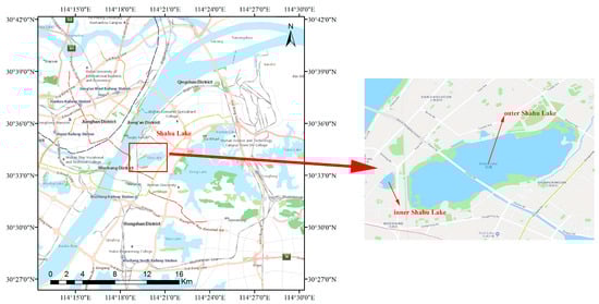
Figure 1.
The geographical location of Shahu Lake in Wuhan, China.
Shahu Lake was once part of a larger water system connected to the East Lake and the Yangtze. The Guangzhou–Wuhan railway, which was constructed in late Qing Dynasty (early 1900s), travels across the lake and physically divides it into two parts, namely the inner Shahu Lake (located in the south, 0.134 km2) and outer Shahu Lake (located in the north, 3.197 km2). The railway line still exists as part of the Beijing–Guangzhou railway, which can be seen from Figure 1 (left map). Therefore, the two parts of the original lake are managed by the local government as individual lakes with different water qualities. Only small rivers and an underground drainage pipe network hydrologically connect them for urban lake ecology.
Shahu Lake is a microcosm of the regional condition, and its centrality within the city of Wuhan brings about a particular set of problems, namely, the lake is perceived as an obstacle for communication and transit as well as an impediment for much needed city expansion. As a consequence, Shahu Lake has experienced continuous shrinking during the past three decades. In particular, the inner Shahu Lake has almost entirely vanished; its surface area is only 0.134 km2 currently. Besides the lake infill, water pollution was serious due to urban waste disposal and domestic sewage discharge. The natural ecology of Shahu Lake was seriously damaged during this period. Not only did many rare birds leave in the past, but also a lot of fish in the lake were killed by the polluted water. According to the statistics from local environmental protection departments in 2006, the water quality of Shahu Lake had the worst grade (class V) of environmental quality standard for surface water (GB3838-2002).
2.2. Data
In order to interpret the Shahu Lake surface extent and land-cover change for this study area, 35 scenes of archived high resolution aerial images covering the study area in different periods were collected from the surveying and mapping department of Hubei province in China, these images were acquired for six separate years from 1978 to 2011, and all of them are cloud free. The characteristics of these images are provided in Table 1.

Table 1.
Characteristics of different aerial images.
The digital aerial photos from 1978 to 2003 were produced from their original aerial film by means of scanning with a high-precision photogrammetric scanner. The last image was generated from digital aerial photography. The img1 was taken in June, while the other five images were acquired in September. According to the accumulated precipitation data from the National Climate Center of China, there was a similar rainfall condition in the study area, without flood and drought in the six years. Therefore, the impacts from climate change on the lake area could be largely ignored.
2.3. Data Pre-Processing
As an essential pre-processing task for image classification and change detection, geometric correction, mosaicking, co-registration, resample and image subsetting were applied to the collected aerial datasets.
Precise geometric registration to a common map reference and co-registration between individual images are crucial for ensuring the reliable detection of temporal changes of land-cover. Initially, all aerial images were geometrically corrected to the universal transverse mercator (UTM) map projection (UTM zone 49 N, WGS-84 geodetic datum). A corrected WorldView-3 satellite imagery with three visible bands (red-green-blue, RGB) at 0.3 m spatial resolution was obtained (taken in October, 2015) and then used as a reference for the image-to-image registration of all aerial images. The registration was done using selected ground control points (GCPs) for each image, and the GCPs were well dispersed throughout the whole study area and yielded root mean square errors (RMSE) of less than 0.8 pixels.
Secondly, all the geo-referenced small aerial images covering the study area of each separate year were mosaicked. In this process, a unifier ray and color of the mosaicked image for each separate year was also done, which plays an important role for further image classification. Thirdly, all the mosaicked images were resampled to the same spatial resolution (1 m). Finally, the resampled six images were then clipped by using the same area of interest (AOI) to cover the whole study area.
The processing of image correction, co-registration, mosaicking, resample and clipping were performed using ERDAS IMAGINE software package (Hexagon Geospatial, Madision, WI, USA). The processed images for each separate year are shown in Figure 2. It can be seen that the study area is characterized by classes of water bodies, built-up area, road, and vegetation (i.e., blocks of farmland on the north side of the lake in Figure 2a–e, scattered trees). There are some yellow bare lands around the lake in Figure 2f.
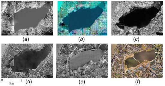
Figure 2.
The mosaicked and geo-referenced aerial images of different years: (a) 1978; (b) 1981; (c) 1989; (d) 1995; (e) 2003 and (f) 2011.
3. Methodology
The methodology of this investigation is summarized and represented in Figure 3.
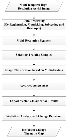
Figure 3.
Schematic representation of the methodology.
The entire workflow includes three major stages: image segmentation, classification, and change detection based on post-classification. Each major stage is subdivided into distinct processing steps, such as building training set, generating decision tree (DT), validating the classification on independent samples, etc.
In this research, object-based image analysis (OBIA) was employed for VHR aerial image classification and change detection due to its advantages over the pixel-based approach, such as adding object shape and context to spectral and textural information, avoiding a “salt-and-pepper” pattern in pixel-based classification [9,22,23]. In the following we summarize the approaches step-by-step for land cover classification and change detection of Shahu Lake with OBIA.
3.1. Multi-Resolution Segmentation
Multi-scale image segmentation is the foundational procedure of OBIA in which the digital image is transformed from discrete pixels into spectrally homogeneous, contiguous image object primitives [24]. Various segmentation techniques have been developed with different results, and the selection of the image segmentation technique may lead to different classification accuracies in OBIA [25]. In this research, all images are partitioned into homogeneous objects through the multi-resolution segmentation algorithm (MRS) within eCognition Developer® software (Trimble, Sunnyvale, CA, USA).
The MRS in eCognition is a widely accepted tool for image segmentation, yet the size of segmented objects is controlled by user-defined scale parameters [26], which means that the selection of segmentation scale parameters is often dependent on subjective trial-and-error methods [27]. As a result, the most typical errors resulting from the segmentation step are under- and over-segmentation [28].
In order to automatically identify the optimal segmentation parameters, the estimation of scale parameter (ESP) tool developed by Drǎguţ et al. is introduced [29], which is based on the idea that the local variance (LV) of object heterogeneity within a scene can indicate the appropriate scale level. The ESP tool iteratively generates image-objects at multiple scale levels in a bottom-up approach and calculates the LV for each scale. Then, variation in heterogeneity was explored by evaluating LV plotted against the corresponding scale. Finally, the thresholds in rates of change of LV (ROC-LV) indicate the scale levels at which the image can be segmented in the most appropriate manner. Moreover, the ESP tool can be integrated with eCognition software suite.
3.2. CART Classification
Over the years, a variety of methods for object-based classification have been developed. Classification and regression trees (CART), introduced by Breiman et al. [30], have become known as the fastest and most versatile predictive modeling algorithm available for analysis and classification. Therefore, this research focuses on a CART-based approach.
CART provides a foundation for important algorithms such as bagged decision trees, random forest and boosted decision trees. The method inherits all the advantages of general decision trees, and can be used to generate accurate and reliable predictive models for a broad range of applications such as image classification [31]. CART trees deliberately restrict themselves to two-way splits of the data, intentionally avoiding the multi-way splits common in other methods. These binary decision trees divide the data into small segments at a slower rate than multi-way splits and thus detect more structure before too few data are left for analysis. Since the method is essentially non-parametric, it has the additional advantage of no necessity in assuming the functional form of the statistical distribution of data.
The representation for the CART model is a binary tree, and each node of the decision tree structure makes a binary decision that separates either one class or some of the classes from the remaining classes. Creating a CART model involves selecting input variables and split points on those variables until a suitable tree is constructed. The selection of which input variable to use and the specific split or cut-point is chosen using a greedy algorithm to minimize the cost function. This is a numerical procedure where all the values are lined up and different split points are tried and tested using a cost function. Tree construction ends up with a predefined stopping criterion, such as a minimum number of training instances assigned to each leaf node of the tree.
Object-based classification in our study is performed with the CART algorithm. Salford Systems’ CART was chosen to generate rule sets for decision tree classification, as it is a robust decision tree tool for data mining, predictive modeling, and data preprocessing. This tool is able to provide reliable performance and accurate results, since there are many advantages for its methodology, such as a powerful binary-split search approach, effective pruning strategy, automatic self-test procedures, cross validation, adjustable misclassification penalties, which help to avoid the most costly errors, etc.
This procedure of CART classifiers requires a set of class-specific training objects from which the distribution of object-level features are obtained to evaluate membership functions of each class. The set of rules defined by the object attributes and their respective thresholds was identified automatically in the SPM® (Salford Predictive Modeler, Salford Systems, San Diego, CA, USA) software suite 8.2, and these rules constitute the DT. The hierarchic classification was then performed according to the DT’s set of rules inside the computational environment of the eCognition software, and a thematic map with different classes of interest was finally produced.
3.3. Change Detection
Once a DT is built it can be used to classify the unknown cases. Change vs. no-change can be treated as a binary-classification problem or a post-classification comparison can be performed to measure the changes. It is perhaps the most commonly used object-based change detection methodology that allows the creation of a change matrix indicating the “from–to” changes. Thus, object-based change detection (OBCD) based on post-classification comparison [32] was employed in this procedure. The classified multi-temporal map objects were compared for a detailed change analysis based on both the geometry and the class membership.
4. Experiment
In order to detect the land use changes at Shahu Lake in the period 1978–2011, a set of experiments on multi-temporary images were carried out using eCognition Developer 9.0 software, including image segmentation, sample selection, classification based on CART, accuracy assessment and change detection.
4.1. Image Segmentation
The optimal segment parameters of scale are defined with the help of the ESP tool. After defining the starting scale parameter as 10, and the step size of the increasing scale parameter as five, the ESP tool iteratively performs multi-scale segmentations of an image with fixed increments of the scale parameter for 200 loops. The results are then exported and analyzed in a LV and ROC-LV graph, which depicts changes in LV (solid red) and ROC (solid blue) with increasing scale parameters (see Figure 4). Finally, a threshold was defined as the first break in the ROC-LV curve after continuous and abrupt decay, i.e., 60 in Figure 4. Drǎguţ et al. [29] had proved that the peaks in an ROC-LV curve indicate the object levels at which the segments delineate their correspondents in the real world, and they tested the ESP tool on a variety of sites. By integrating the ESP tool with the eCognition software, the selection of scale parameters was performed for each scene, and we further confirmed that the selected scale parameters are appropriate by visual comparison and the assessment of different segmentation results. During the identification of suitable scale parameters in the ESP tool, the other parameters shape and compactness were set as 0.3 and 0.5 respectively according to the description in [33] and the suggestion in [29].
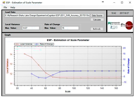
Figure 4.
ESP (estimation of scale parameter) tool output for the 2011 image.
Once the proper scale parameter for each image had been identified, the multi-resolution segmentation tool was applied to segment the six images into meaningful objects for the classification procedure. These segmentation parameters for the six images are presented in Table 2. The scale of the first image was greater than the others, mainly because there were many large homogenous areas in this image, and a high scale parameter would benefit the extraction of large features and the creation of meaningful objects for classifying specific features.
Table 2.
The optimal segment parameters used for each aerial image.
4.2. Sample Selection
To generate the independent set of training and testing samples and to ensure representative sampling coverage of the entire study area, a skilled expert classified more than 7500 samples (objects) through the visual interpretation of a temporal series of aerial images that were selected. There were a total of 2719 training samples and 5205 testing samples, including five land cover types: water (lake and river), vegetation (tree, grass and farm land), bare land, building, and road. There were fewer training objects so as to avoid redundant training samples.
The training and testing sample count of each class for these images are reported respectively in Table 3 and Table 4.
Table 3.
The training samples used for each aerial image.
Table 4.
The testing samples used for each aerial image.
4.3. CART Classification
During the classification processing, firstly the selected training samples were exported in vector format with features in an attribute table. Then, these features were used to train the CART model to identify patterns. Figure 5 illustrates an example of the binary decision tree generated by SPM CART modelling on the training set.
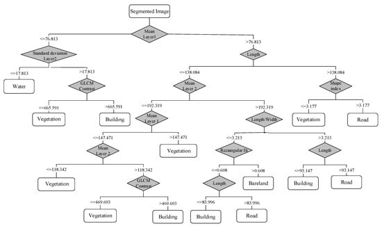
Figure 5.
A decision tree constructed for the segmented 1981 image.
Since features extracted from the image objects are often of high dimension and highly correlated, the classification algorithms frequently used in OBIA do not perform well if all object features are used in the classification. Therefore, feature selection is also important for classification. We can see that only seven dimensions of the feature space are identified to separate different classes in Figure 5, which are spectral features (mean, standard deviation), shape features (length, length/width, shape index, rectangular fit), and texture features (gray-level co-occurrence matrix (GLCM) contrast (all directions)).
It can be seen that the water class can be firstly distinguished by its spectral behavior (mean, standard deviation). Bare land could be identified by four attributes: mean, length, length/width, and rectangular fit. The classification of buildings and vegetation is difficult because they are represented by various features, so more indices such as GLCM contrast are introduced to separate them from other classes.
Different decision trees with individual sets of rules were built so as to facilitate the best discrimination of classes based on the training samples from each separate image. Then, these decision trees generated in SPM were implemented in eCognition Developer, by converting the decision rules into thresholds for various attributes. Each separate image was then classified into water, vegetation, bare land, farmland, building and road using the CART classifier. The final classification results of these images are shown in Figure 6. For the 2011 image, there were seven classes, including building shadow, which was presented in black color.
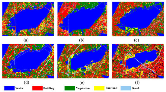
Figure 6.
The classification results based on CART (classification and regression trees): (a) 1978; (b) 1981; (c) 1989; (d) 1995; (e) 2003 and (f) 2011.
4.4. Accuracy Assessment
In order to evaluate the classification accuracy in a more objective manner, an accuracy assessment was carried out. The accuracy of these images was estimated based on testing samples carefully selected from each individual image. The validation samples were partitioned to 10 × 10 pixels size with a chessboard segmentation algorithm, these small objects were then applied to calculate the confusion matrix.
The classification result of each separate image was quantitatively assessed through the overall accuracy and Kappa coefficients, both extracted from the confusion matrix. The quantitative statistic was reported in Table 5, and it can be seen that an average of 92.07% overall accuracy was achieved, and the mean Kappa coefficient was 0.8909.
Table 5.
Overall accuracy for each aerial image.
4.5. Change Detection
The six independently classified images were then run for post classification comparison in order to produce a change detection analysis, which was conducted using ArcGIS 10.3. The outputs of the decision tree classifier were overlaid to produce the land use changes in a time-series starting from 1978 to 2011. The surface area change of Shahu Lake between different periods is reported in Table 6, and the last column indicates the change in total area with respect to the previous year. Since there is a bridge across the lake in the last image, the portion of the bridge over the lake was considered as water while computing the lake area. The results show that the total area of Shahu Lake has been reduced from ~7.64 km2 to ~3.60 km2 over the past 33 years, which indicates that this lake had experienced rapid shrinking during this period. The most intense changes in Shahu Lake were detected between 1995 and 2003, during which the lake lost ~34.83% of its surface area in comparison with the year 1978 and 33.40% of its surface area in comparison with the year 1995. From 2003 to 2011, the shrinking of this lake can also not be ignored, as there was more than 1.38 km2 of lake area lost in this period. The outer lake lost 49.17% (3.4186 km2) of its original surface extent from 1978 to 2011, whereas 90.81% (0.6219 km2) of the inner lake surface was damaged during these years, and it has almost disappeared.
Table 6.
The area statistics of Shahu Lake.
In order to investigate what led to the intense shrink of Shahu Lake between 1995 and 2003, a “from–to” change map was obtained based on the two classification results, which is shown in Figure 7a. The post-classification comparison showed that the lost lake surface area has been replaced by a large number of buildings, bare lands, vegetation, and roads. Similarly, another land cover change map of the Shahu Lake surface from 1978 to 2011 is presented in Figure 7b, which indicates that the built-up area, including buildings and roads, had the maximum impact on the losses of lake areas during this period.
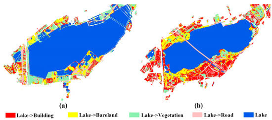
Figure 7.
The post-classification change detection results in different periods: (a) 1995–2003, and (b) 1978–2011.
The area coverage and changes of the LC categories are summarized in Table 7, which represents the large increment in the coverage of roads and building areas, in particular the area with buildings has increased by more than two times. The lake and vegetation lost over 40 percent of their original areas. The significant decline in the lake coverage between 1978 and 2011 is clearly the result of the rise of mass construction. Therefore, it is some of the best evidence of lake shrinking due to rapid urbanization.
Table 7.
The area coverage and changes of the land cover categories between 1978 and 2011.
5. Discussion
The generated classification and statistics results revealed a significant change in the surface area of Shahu Lake over its history, and these changes confirm different human-made external driving forces in the watershed area. The total area of this lake increased a little between 1978 and 1981 due to the fact that some farmland was flooded, since the 1981 image was captured after rainfall. The rapid urbanization since the 1980s has completely encapsulated the lake with high-rise buildings, hiding the lake behind a forest of concrete slabs. Shahu Lake changed little before 1995, since the urbanization was still in the initial stages during these 17 years. In the 1990s, some roads around Shahu Lake were built or widened at the cost of filling part of this lake, since the famous Second Wuhan Yangtze River Bridge was built. Meanwhile, as urbanization intensified, the lake continues to be devoured by real estate development and other damages, especially during the period from 1995 to 2011. During the 17 years from 1995 to 2011, the local government attached great importance to economic and urban development, as a result, more than half of Shahu Lake’s surface area was filled with dirt to make land, which can be seen in Table 6. Moreover, due to great quantities of wastewater from factories and the construction industry being discharged into the lake, the pollution of the lake was also becoming more and more serious, which led to the prohibition of fish farming in Shahu Lake since 2007.
Shahu Lake has shrunk a great deal over the past few decades, due to rapid urbanization and to imperfect legislation for the protection of the lake. To strengthen the protection of lakes in Wuhan, and to prevent the occupation of and damage to the existing lakes, the Lake Protection Regulations of Wuhan were promulgated by local government on 1 March 2002. Since then, the occupation of Shahu Lake has been reduced a lot, and the lost area of this lake during the period from 2003 to 2011 was less than the previous eight years. However, Shahu Lake was still shrinking due to rapid urbanization, which indicates that the legislation for the protection of these lakes was not perfect. Thus, the governments of Wuhan began to take more stringent measures to strengthen the protection and management of urban lakes. In December 2012, a lake protection plan of “three lines and one way” in the center city of Wuhan was made by Wuhan Land Resource and Planning Bureau. The three lines are the lake water protection line (blue line), the lake green control line (green line), and the waterfront construction control line (gray line). “One way” stands for the road around the lake, including a car path and walking path around the lake. The three lines of the Outer Shahu Lake protection plan are shown in Figure 8. The blue line indicates the surface extent of the Shahu Lake watershed, and it is the boundary of the lake water ecological protection. The green line identifies the transition between the water ecosystem and urban terrestrial ecosystem, while the gray line is the boundary of the construction control area for the protection of the sharing and heterogeneity of the water environment.
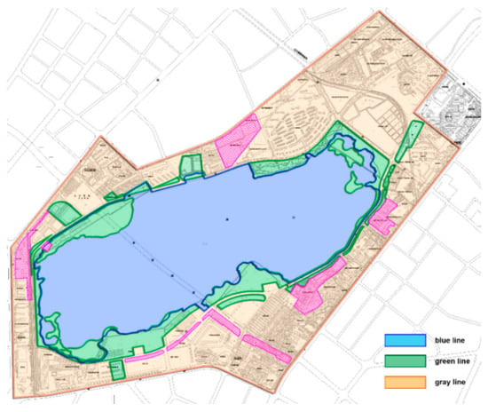
Figure 8.
The three lines of Outer Shahu Lake protection plan.
The areas controlled by blue line, green line and gray line are 3.078 km2 (307.8 hectare), 0.901 km2, 3.918 km2, respectively. The length index controlled by the blue line is 9.8 km. There is a similar figure for the protection plan of the inner Shahu Lake, and the area and length controlled by the three lines for the two lakes are described in Table 8. The surface extent of Outer Shahu Lake will remain at 3.078 km2, while the extent of Inner Shahu Lake will not be less than 0.056 km2.
Table 8.
Area and length indices controlled by the three lines of the Shahu Lake protection plan.
Beside this protection plan, the local government revised the lake protection regulations on 1 June 2015, so as to prevent further damage to the existing lakes. It can be seen from these policies that the protection of urban lake resources comes first in the new round of urbanization in Wuhan.
On the other hand, to improve the water quality of Shahu Lake and the drainage capacity of this region, the Chu River and Han Street was developed by the end of September 2011, which was a project of the first phase of the Wuhan Central Cultural Zone. Chu River, as a water channel of 2.2 km in length, connects the East Lake and the Shahu Lake in Wuhan, and it is the first of the “lake linking plan” for water network treatment projects approved by the State Council of China. In addition, the Shahu Bridge across the Shahu Lake was built as one part of this project, which did not damage the existing water environment of the Outer Lake. Thus, there is a small river that appears in the lower right corner of the last image, and a long road across the lake area. Shahu Lake is no longer subject to any damage under these strict measures of protection. In addition, a new open Shahu Park with the characteristics of historical culture and a wetland landscape has been gradually built since 2009, and the lake ecosystem has been significantly improved, especially the water quality of the inner lake.
6. Conclusions
Land cover mapping and change detection have increasingly been recognized as one of the most effective tools for environmental resource management. This study showed the use of multi-temporal VHR images to perform a detailed change analysis based on OBIA techniques with respect to special areas of interest. We have demonstrated that significant changes in land-use and land cover have occurred along with the rapid urbanization during 1978–2011. The dominant changes that took place in the study area during this period were lake and vegetation shrinking, being replaced by built-up areas, such as high density buildings and roads.
The utilization of automated segmentation algorithms to delineate polygons, coupled with CART modelling to develop rules to supervise classification, brought a high accuracy and consistency to the final product that has not been obtainable using manual image interpretation. These classification results showed high levels of exactitude, with the average overall accuracy and the Kappa coefficients reaching 92.07% and 0.89, respectively. It must be pointed out that perfect classification results come from all classification processing, including not only the classification algorithm, but also image pre-processing, sample selection and post-processing.
Our study clearly demonstrated the benefits of the rapid and accurate change detection using VHR images acquired on different dates. Post-classification change detection based on multi-temporal imagery made a successful change analysis with respect to the landscape of Shahu Lake. It can be stated that the proposed methodology enables us to better understand the spatial changes of Shahu Lake in detail on the one hand, and the trends of urban growth on the other hand. Currently, the local authorities are paying growing attention to the dynamic monitoring of urban lakes based on high resolution remote sensing images from sensors like WorldView and Gaofen-3, and this technology has made remarkable achievements in the discovery of illegal urban lake filling. Future studies may include vector dataset and social economic data in order to perform more detailed change analysis, and assist the local government in making more scientific and reasonable urban lake protection plans.
Acknowledgments
This work was supported by the National Key Technologies R&D Program of China (2012BAH83F00). The authors would like to thank Lv Zhiyong from the computer school of Xi’An University of Technology for providing us with valuable suggestions on the change detection approaches. We also greatly appreciate the reviewers for their constructive comments which helped to enhance the quality of the article.
Author Contributions
Wenyuan Zhang wrote the paper; Guoxin Tan conceived and designed the experiments; Songyin Zheng and Wenyuan Zhang performed the experiments; Chuanming Sun analyzed the data. Xiaohan Kong and Zhaobin Liu did part of image processing and provided some hydrology information.
Conflicts of Interest
The authors declare no conflict of interest.
References
- Zhu, J.; Zhang, Q.; Tong, Z. Impact analysis of lakefront land use changes on lake area in Wuhan, China. Water 2015, 7, 4869–4886. [Google Scholar] [CrossRef]
- Snehal, P.; Unnati, P. Challenges faced and solutions towards conservation of ecology of urban lakes. Int. J. Sci. Eng. Res. 2012, 3, 170–183. [Google Scholar]
- Zhu, W.; Jia, S.; Lv, A. Monitoring the fluctuation of lake Qinghai using multi-source remote sensing data. Remote Sens. 2014, 6, 10457–10482. [Google Scholar] [CrossRef]
- Taravat, A.; Rajaei, M.; Emadodin, I.; Hasheminejad, H.; Mousavian, R.; Biniyaz, E. A spaceborne multisensory, multitemporal approach to monitor water level and storage variations of lakes. Water 2016, 8, 478. [Google Scholar] [CrossRef]
- Zhu, Z.; Woodcock, C.E. Continuous change detection and classification of land cover using all available Landsat data. Remote Sens. Environ. 2014, 144, 152–171. [Google Scholar] [CrossRef]
- Demir, B.; Bovolo, F.; Bruzzone, L. Updating land-cover maps by classification of image time series: A novel change-detection-driven transfer learning approach. IEEE Trans. Geosci. Remote Sens. 2013, 51, 300–312. [Google Scholar] [CrossRef]
- Volpi, M.; Petropoulos, G.P.; Kanevski, M. Flooding extent cartography with Landsat TM imagery and regularized kernel Fisher’s discriminant analysis. Comput. Geosci. 2013, 57, 24–31. [Google Scholar] [CrossRef]
- Bagan, H.; Yamagata, Y. Landsat analysis of urban growth: How Tokyo became the world’s largest megacity during the last 40years. Remote Sens. Environ. 2012, 127, 210–222. [Google Scholar] [CrossRef]
- Dronova, I.; Gong, P.; Wang, L. Object-based analysis and change detection of major wetland cover types and their classification uncertainty during the low water period at Poyang Lake, China. Remote Sens. Environ. 2011, 115, 3220–3236. [Google Scholar] [CrossRef]
- Rokni, K.; Ahmad, A.; Selamat, A.; Hazini, S. Water feature extraction and change detection using multitemporal landsat imagery. Remote Sens. 2014, 6, 4173–4189. [Google Scholar] [CrossRef]
- Foody, G.M. Status of land cover classification accuracy assessment. Remote Sens. Environ. 2002, 80, 185–201. [Google Scholar] [CrossRef]
- Woodcock, C.E.; Allen, R.; Anderson, M.; Belward, A.; Bindschadler, R.; Cohen, W.; Gao, F.; Goward, S.N.; Helder, D.; Helmer, E.; et al. Free access to Landsat imagery. Science 2008, 320, 1011–1012. [Google Scholar] [CrossRef] [PubMed]
- Zheng, Z.; Li, Y.; Guo, Y.; Xu, Y.; Liu, G.; Du, C. Landsat-based long-term monitoring of total suspended matter concentration pattern change in the wet season for Dongting Lake, China. Remote Sens. 2015, 7, 13975–13999. [Google Scholar] [CrossRef]
- Michishita, R.; Jiang, Z.; Xu, B. Monitoring two decades of urbanization in the Poyang Lake area, China through spectral unmixing. Remote Sens. Environ. 2012, 117, 3–18. [Google Scholar] [CrossRef]
- Song, C.; Huang, B.; Ke, L. Modeling and analysis of lake water storage changes on the Tibetan Plateau using multi-mission satellite data. Remote Sens. Environ. 2013, 135, 25–35. [Google Scholar] [CrossRef]
- McFeeters, S.K. The use of the Normalized Difference Water Index (NDWI) in the delineation of open water features. Int. J. Remote Sens. 1996, 17, 1425–1432. [Google Scholar] [CrossRef]
- Feyisa, G.L.; Meilby, H.; Fensholt, R.; Proud, S.R. Automated Water Extraction Index: A new technique for surface water mapping using Landsat imagery. Remote Sens. Environ. 2014, 140, 23–35. [Google Scholar] [CrossRef]
- Zhu, Z.; Woodcock, C.E. Object-based cloud and cloud shadow detection in Landsat imagery. Remote Sens. Environ. 2012, 118, 83–94. [Google Scholar] [CrossRef]
- Chen, G.; Hay, G.J.; Carvalho, L.M.T.; Wulder, M.A. Object-based change detection. Int. J. Remote Sens. 2012, 33, 4434–4457. [Google Scholar] [CrossRef]
- China Online Community (MapServer). Available online: http://cache1.arcgisonline.cn/ArcGIS/rest/services/ChinaOnlineCommunityENG/MapServer (accessed on 16 November 2017).
- Google Map. Available online: http://www.google.cn/maps/@30.5641107,114.3232634,16.75z?hl=en (accessed on 12 November 2017).
- Laba, M.; Blair, B.; Downs, R.; Monger, B.; Philpot, W.; Smith, S.; Sullivan, P.; Baveye, P.C. Use of textural measurements to map invasive wetland plants in the Hudson River National Estuarine Research Reserve with IKONOS satellite imagery. Remote Sens. Environ. 2010, 114, 876–886. [Google Scholar] [CrossRef]
- Zhong, Y.; Zhao, J.; Zhang, L. A hybrid object-oriented conditional random field classification framework for high spatial resolution remote sensing imagery. IEEE Trans. Geosci. Remote Sens. 2014, 52, 7023–7037. [Google Scholar] [CrossRef]
- Ming, D.; Li, J.; Wang, J.; Zhang, M. Scale parameter selection by spatial statistics for GeOBIA: Using mean-shift based multi-scale segmentation as an example. ISPRS J. Photogramm. Remote Sens. 2015, 106, 28–41. [Google Scholar] [CrossRef]
- Hussain, M.; Chen, D.; Cheng, A.; Wei, H.; Stanley, D. Change detection from remotely sensed images: From pixel-based to object-based approaches. ISPRS J. Photogramm. Remote Sens. 2013, 80, 91–106. [Google Scholar] [CrossRef]
- Anders, N.S.; Seijmonsbergen, A.C.; Bouten, W. Segmentation optimization and stratified object-based analysis for semi-automated geomorphological mapping. Remote Sens. Environ. 2011, 115, 2976–2985. [Google Scholar] [CrossRef]
- Belgiu, M.; Drǎguţ, L. Comparing supervised and unsupervised multiresolution segmentation approaches for extracting buildings from very high resolution imagery. ISPRS J. Photogramm. Remote Sens. 2014, 96, 67–75. [Google Scholar] [CrossRef] [PubMed]
- Liu, D.; Xia, F. Assessing object-based classification: Advantages and limitations. Remote Sens. Lett. 2010, 1, 187–194. [Google Scholar] [CrossRef]
- Drǎguţ, L.; Tiede, D.; Levick, S.R. ESP: A tool to estimate scale parameter for multiresolution image segmentation of remotely sensed data. Int. J. Geogr. Inf. Sci. 2010, 24, 859–871. [Google Scholar] [CrossRef]
- Breiman, L.; Friedman, J.; Stone, C.J.; Olshen, R.A. Classification and Regression Trees; Chapman and Hall CRC: New York, NY, USA, 1984. [Google Scholar]
- Lawrence, R.; Bunn, A.; Powell, S.; Zambon, M. Classification of remotely sensed imagery using stochastic gradient boosting as a refinement of classification tree analysis. Remote Sens. Environ. 2004, 90, 331–336. [Google Scholar] [CrossRef]
- Blaschke, T. Towards a framework for change detection based on image objects. Göttinger Geogr. Abh. 2005, 113, 1–9. [Google Scholar]
- Benz, U.C.; Hofmann, P.; Willhauck, G.; Lingenfelder, I.; Heynen, M. Multi-resolution, object-oriented fuzzy analysis of remote sensing data for GIS-ready information. ISPRS J. Photogramm. Remote Sens. 2004, 58, 239–258. [Google Scholar] [CrossRef]
© 2018 by the authors. Licensee MDPI, Basel, Switzerland. This article is an open access article distributed under the terms and conditions of the Creative Commons Attribution (CC BY) license (http://creativecommons.org/licenses/by/4.0/).