Economic Feasibility of Underwater Adduction of Rivers for Metropolises in Semiarid Coastal Environments: Case Studies

Abstract

The supply of raw water to the inhabitants of metropolises is not a trivial problem, and involves many challenges, both in terms of the quantity and quality of this water. When these metropolises are located in semiarid regions, this challenge takes on enormous proportions, and in many situations, there are no sustainable solutions, especially in times of global climate change. One hypothesis to try to mitigate this problem in coastal cities is the underwater adduction of rivers. The objective of this paper was to make the abstraction of drinking water in the mouths of great rivers near semi-arid regions. This water would be led by a pipeline below the water level and would follow the route of the seacoast, where the energy to move the water would be supplied by an axial hydraulic pump embedded in the pipeline by water-cooled electric motors driven by the energy generated from offshore wind turbines. Estimates have been made for the four metropolises in semi-arid regions: Fortaleza-Brazil, Dalian-China, Tel Aviv-Israel, and Gaza-Palestine, where it was possible to calculate economic viability through the Present Worth Value, the internal rate of return, and payback. The results indicated that Fortaleza had economic viability under restrictions. Dalian proved the ideal result. Tel Aviv and Gaza both had great economic viability, but only if Egypt agreed to supply water from the Nile. This paper proved that the management of the water supply for human consumption through the underwater adduction of rivers could be achieved with real clearance for any deficits in the volume of water that due to global climate change are becoming more frequent.

1. Introduction

A major problem for human populations in semi-arid environments is the lack of water for domestic consumption. On average, a person needs 200 L of water [1] per day to meet their basic needs. In situations of water scarcity, this volume is lower, and according to [2], it ranges from 50 (intermediate access) to 100 (optimum access) L per capita per day; in emergency situations, the value is 20 L per capita per day. The authors in [3] affirmed that 81 L per capita per day was sufficient for one non-agricultural economy that used water efficiently. These volumes of water per person are very difficult to obtain in environments where the average annual rainfall is low (less than 800 mm), a value that characterizes the semi-arid environment [4]. This difficulty is even more important when considering that the rivers that exist in these environments are not permanent but go through periods without flow and the occurrence of a dry period has a probability greater than 60% [4].

In this context, a major challenge for governments is to enable the supply of water for domestic consumption in urban communities that are located in semi-arid environments, especially in the context of global climate change. In some semi-arid regions climate change can even be beneficial, According to [5] in China, northern boundaries of multiple cropping systems have been shifted northward due to climate change and the projected China’s crop planting areas for triple-cropping system would expand and multiple cropping systems would increase national cereal production, but in general climate change it is a big problem. For example, Israel is highly sensitive to the potential impacts of this phenomenon, with increases in temperature and decreased precipitation [6]; Northeastern Brazil has declining rainfall and rising temperatures [7]; and Northwestern China (Yellow River Basin) may decline by up to 25.7% runoff [8].

A water supply system consists of a water source, water treatment in water treatment plants, and storage and distribution to the consumer. This challenge is important when considering cities with hundreds of thousands, sometimes many millions of inhabitants, which directly represent the supply of millions of cubic meters of drinking water. This geopolitical situation demands large investments in infrastructure that may become useless or uneconomical if there are changes to the weather patterns.

The environmental planning process in terms of water supply systems in cities in these regions is complex and not trivial. This situation arises due to the stochastic seasonality of rainfall, a fact that brings years with plenty of water, and others with long lasting droughts [9]. This characteristic is exacerbated as the randomness of rainfall is increasing due to global climate change [10].

Coastal areas that have water “imported” or underground resources are suffering an increase of cuts in water supply due to changes in the weather patterns, which has generated recurrent droughts [11]. The increase in the stochastic characteristic of rainfall in semiarid regions has generated lasting drought, for example, the drought in Northeastern Brazil in 2013, which was the most severe in 50 years [12].

Some of the solutions to solve the water supply problem for human consumption in cities include: (1) Storage in reservoirs; (2) Use of groundwater; (3) Desalinization of seawater; and (4) Inter-Basin Water Transfer.

In relation to water storage in reservoirs, this type of water supply system is very sensitive to climate change, which has seen more frequent severe droughts, thus the recharge of the reservoirs is being impaired mainly in extreme events [13]. Climate change is affecting populations in coastal environments around the world, especially in areas in tropical and subtropical regions to the south of the planet, so it is important to start developing disaster plans and detailed studies on drinking water as there is a serious concern about the supply of water to the population [14].

Regarding the use of groundwater sources under the soil, this method has a strategic place in times of climate change, mainly because aquifers can provide water for long periods, even during long and severe droughts [15]. In some coastal areas and islands, the reliance on groundwater sources is immense [16]. However, a major problem is intruded salt water into the coastal aquifers, especially when increasing the use of these resources in arid environments, which leads to overexploitation and saltwater intrusion [17]. According to [18], the overexploitation of groundwater has positive effects such as the re-infiltration of excess irrigation water with the recharge of the aquifer, recovery of saline soils, increase in vegetation cover, change from a non-irrigated to an irrigated regime. Nevertheless, over time the effects become increasingly negative including continuous failure in piezometric levels with increased costs for the continuous failure in piezometric levels with increased costs of pumping; the abandonment of wells; diminishing groundwater reserves; induced compaction of the land surface; change in the physical and chemical characteristics of the groundwater; modification induced in the river flow regime; impact or desiccation of wetlands and springs; and changes in the groundwater extraction systems.

In terms of the provision of drinking water through the desalination process, the use of water from desalination processes is increasing in arid regions due to increased water demand from population growth, the industrial expansion, tourism, and agriculture [19]. In general, desalinization is not a universal solution for fresh water supply in all regions with water scarcity as it is cost prohibitive [19]. There are three issues with desalination: the desperate need to meet demand; dramatic improvement in the energy consumption of modern systems; and reducing costs in desalination processes [20].

The transfer of inter-basin water is when rainfall is higher in a watershed and the need is greater in another; in this context a solution is interconnection between basins, however, this can cause environmental damage to the involved basin [21] as any inter-basin transfer generates complex phenomena (physical, chemical, biological, and hydrological) in these changed systems [22]. The transfer of inter-basin water is designed to ensure access to this feature through artificial water transport to locations where people need it; this action is typically an engineering measure oriented to meet the demand and causes major social challenges [23].

Based on the above discussion, it is clear that the debate on water supply systems in semi-arid areas in coastal environments is not over. For each proposed conventional solution, there are difficulties and restrictions, which indicate the need for innovative ideas. Innovation refers not only to new products, results, and processes introduced in the world (absolute innovation), but also includes existing techniques that are used of new ways (diffusion).

An innovative solution has been the use of submarine pipelines to import water to islands from nearby continents or larger islands with available water in Seychelles, Malaysia and China [24]. Recently, the construction of an 80 km long undersea pipeline of 1600 mm in 250 m depth in the Mediterranean was achieved to transfer water from the Anamurium Plant in Turkey to the Güzelyalı Pumping Station in Northern Cyprus has made underwater adductions a realistic option for transboundary drinking water transfers [25].

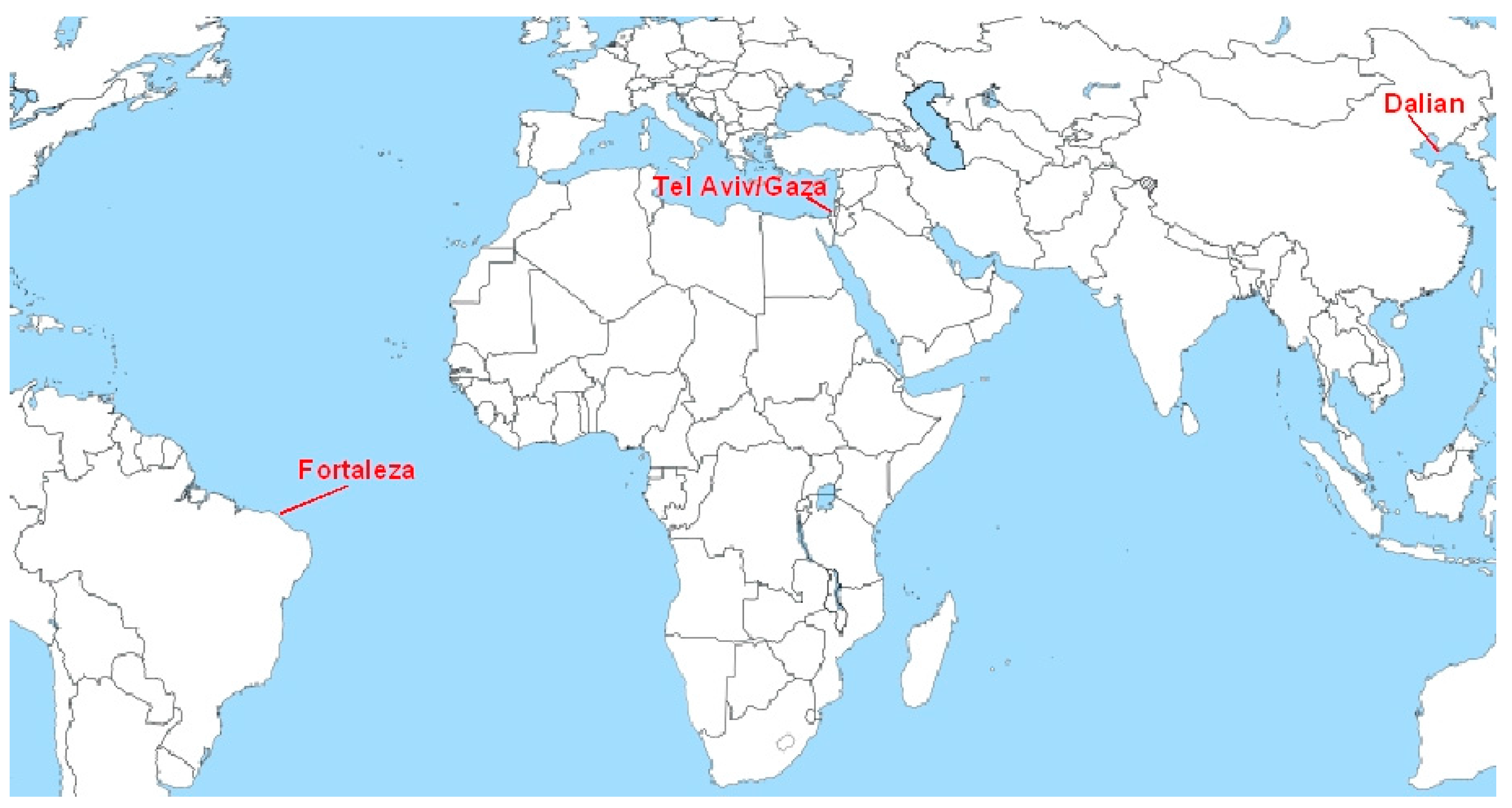
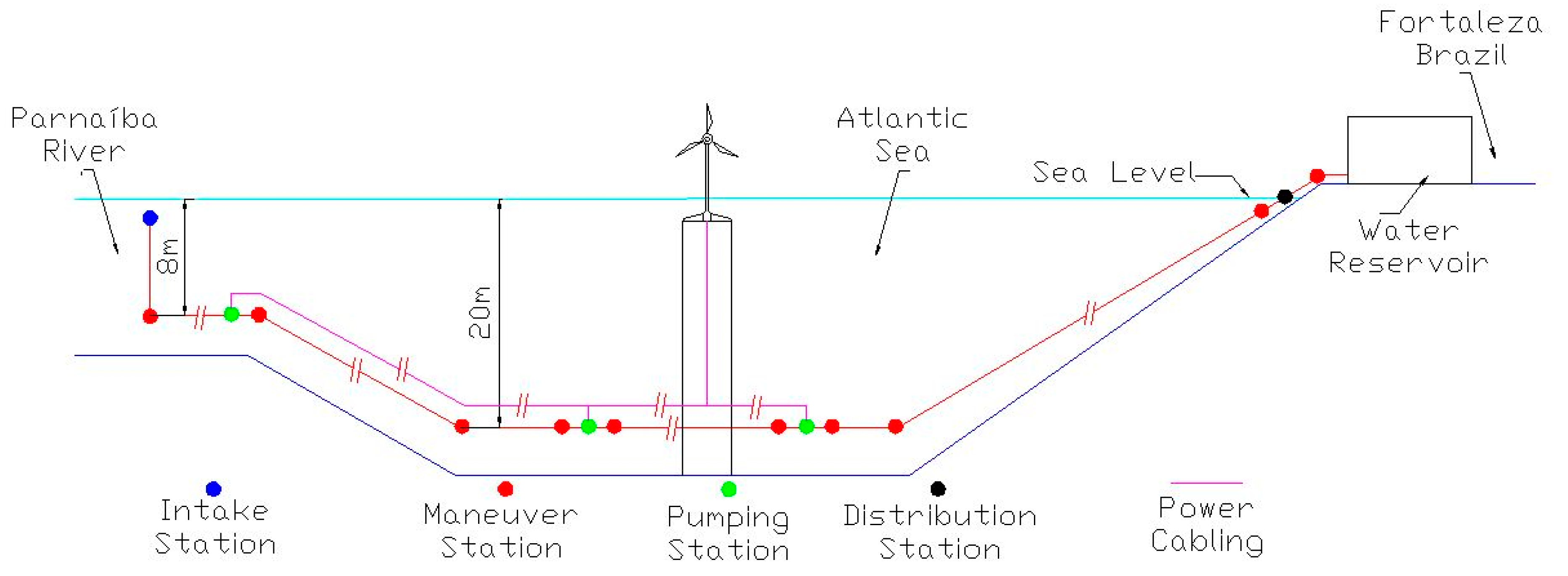
In trying to provide an innovative proposal, this paper proposed a solution to the water supply of cities in coastal semi-arid environments through the underwater adduction of rivers. The idea was to make the abstraction of drinking water in the mouths of great rivers near the semi-arid regions. This water would be led by a pipeline below water level that would follow the route of the seacoast, where the energy to carry the raw water would be supplied by wind turbines offshore.

2. Materials and Methods

Four metropolitan regions were chosen due to their location in semi-arid regions that suffer the negative effects of climate change, and also because they have a population of several million people: Fortaleza, Brazil; Tel Aviv/Gaza, Israel/Palestine; and Dalian, China. The rivers used for drinking water were the Parnaiba in Brazil; the Nile in Egypt, and the Huanghe in China. All intakes were allocated at the mouths of their rivers. Two scenarios were calculated for water demand: (1) scenario 200 L per capita per day; and (2) scenario 81 L per capita per day. The data of the metropolitan regions and characteristics of rivers are in

Table 1. Regions Metropolitan and Rivers chosen.

Metropolis Name	Number of Municipalities	Area (km2)	Number of Inhabitants (Thousands of Person)	Water Demand Scenario 1 * (m3/s)	Water Demand Scenario 2 + (m3/s)
Fortaleza a	19	7440	3985	9.34	3.73
Tel Aviv b	254	1516	3713	8.59	3.48
Gaza c	5	365	1850	4.28	1.73
Dalian d	10	12,584	5943	13.75	5.57

Notes: ^a [26]; ^b [27]; ^c [28]; ^d [29]. * [1] Consumption of 0.2 m³/person/day.⁺ [3] Consumption of 0.081 m³/person/day.

and

Table 2. Characteristics of Rivers chosen.

River Name	Speed Flow * (m/s)	Suspended Solids # (g/L)	Turbididty (max-min) & (NTU) +	Mean Flow % (m3/s)
Parnaíba 1	1.00	0.34	(150-5)	763
Nilo 2	1.48	1.80	(100-20)	2830
Huanghe 3	2.20	3.34	(200-150)	1997

Notes: * 1-[30]; 2-[31]; 3-[32]; ^# 1-[33]; 2-[34]; 3-[35]; ^& 1-[36]; 2-[34]; 3-[37]; ^% 1-[38]; 2-[39]; 3-[40]. ⁺ Nephelometric Turbidity Unit.

.

According to [41], the turbidity limit of water for human consumption is 5 NTU, therefore for the data presented in Table 2, all rivers were above the defined threshold. This suggests that specific procedures must be adopted for treatment stations to decrease the turbidity of the water such as coagulation and flocculation, but the goal of this project was to check only the transport of the raw water, not the considerations on the treatment plant, which is considered to be the end customer of the pipeline.

The location of each city is displayed in the world map in Figure 1.

2.1. Location of Underwater Pipes

To locate underwater pipes, we chose a path that optimized the consumption of materials and at the same time made possible the proper conformation on the coastline between the river mouth, and the delivery point in the metropolis. Special attention was given to the sea routes that were intercepted by the pipeline, which determined the depth of the underwater pipe. Maps were used with the bathymetry of the seabed and included the defined depths of underwater pipes: Parnaíba/Fortaleza, Brazil, 20 m; Huanghe/Dalian, China, 20 m; and Nile/Tel Aviv, Gaza, Israel, Palestine, 50 m due to the crossing of access routes to the Suez Canal.

According to [42], water containing Total Dissolved Solids (TDS) concentrations below 1000 mg/L is usually acceptable to consumers. The palatability of drinking water has been considered as good between 300 and 600 mg/L [43]. The problems with brackish water was avoided due to the location of the water intake of systems far from the shoreline, inside the mouths.

According to [44], at the mouth of the Rio Parnaíba, the TDS ranged between 29 and 30 mg/L, so the pipeline intake was allocated 1000 m inside the mouth. The authors in [45] reported that at the bifurcation between the branches Damietta and Rosetta of the Nile (approximately 150 km from the coast) the TDS ranged between 179 and 259 mg/L, so the system admission was allocated 30 km inside the Rosetta branch. Reference [46] estimated that the Practical Salinity Unit (PSU) of the Huanghe at 30 km from the mouth varied between 0.1 and 0.2 PSU, which is approximately equivalent to a TDS of 100 to 200 mg/L, so the system was allocated 30 km inside the mouth of the Huanghe.

The locations of the pumping systems (Figure 2, Figure 3 and Figure 4) were divided into sections for ease of installation and maintenance of the pumping units, as well as the location of offshore wind farms.

The wind farms were allocated in the best wind conditions for generating electricity. The wind maps are shown in Figure 5, Figure 6 and Figure 7.

2.2. Methodology for Calculation of Underwater Pipes

There are several methodologies for calculating the diameter of pipelines: flow rate, based on normalized flow velocity values [51]; the cost of pipes, based on the linear variation of cost and the derivation of the cost function to find the minimum value [51]; the weight of the pipe based on the derivation of the diameter of the pipe for to obtain the optimal weight in economic terms [52]; economic discharging speed, based on the derivation of the total annual cost function [53]; the Bresse formula based on flow rate, pipe type, and flow velocity that must be used in a continuous operation system (24 h) is the simplest methodology although with a high degree of uncertainty, being ideal for a first approximation [1].

The calculation of underwater pipes followed the recommendations of [1], considering the calculation procedure for pipelines in penstock. It was chosen as the methodology given by the Bresse equation:

$$D=k\sqrt{Q}$$

(1)

where D is the diameter of pipeline (m); k is a constant (in this paper it was adopted as 1.2 [1]); Q is the adducted flow (m³/s).

The continuous head losses were calculated in the universal equation of head losses:

$$\Delta h=\frac{f{U}^{2}l}{2gD}$$

(2)

where Δh is the overall head losses (m); f is the coefficient of head losses; U is the mean flow speed (m/s); D is the diameter of the pipeline (m); g is the gravity acceleration (9.8 m/s²); and l is the length of the pipeline (m).

The localized head losses were calculated for the following equation:

$$\Delta h^{″}=\frac{K{U}^2}{2g}$$

(3)

where Δh″ is the localized head losses (m); K is the coefficient of localized head losses, depending on the Reynolds number and geometry of singularity.

The schematic diagram of the underwater adduction line to the metropolis of Fortaleza, Brazil is shown in Figure 8.

The concept of the underwater pipeline forms in an intake station, a distribution station, several pumping stations, and maneuver stations. The pipe is made of reinforced concrete pipes with a characteristic strength of concrete (fck) of 25 MPa and steel CA50 (yield tension of 500 MPa) with an external polyethylene coating. Axial hydraulic pumps set the pumping stations; maneuver stations have butterfly valves and relief valves. There are also security systems from the water hammer and all pumping and maneuvering stations with relief valves and hydropneumatics reservoirs. The pipe installation on the seabed can be done by a specially adapted wind turbine installation vessel. Due to a large number of suspended solids in the Huanghe River, it needs a sand trap on admission at the river mouth and another in the delivery of water in Dalian.

The hydraulic transients were calculated according to the methodology described by [1]. If pressure waves were considered elastic so the speed was longer than the critical time, the hydraulic transient was reduced. The critical time was calculated based on celerity:

$$C=\frac{\sqrt{\frac{J}{\rho }}}{\sqrt{1+\frac{JD\Phi }{Ee}}}$$

(4)

where C is the celerity, the effective speed of propagation of the pressure wave (m/s); J is the volumetric elasticity modulus of water (2.24 × 10⁸ N/m²); ρ is the specific mass of water at 20 °C (1018 kg/m³); D is the diameter of the pipe (m); e is the thickness of the pipe (m); E is the modulus of elasticity of the material pipe ; concrete (2.38 × 10⁷ Pa); Φ the coefficient of fixing the pipe, expansion joins between anchorages, where $\mathsf{\Phi }=1-\frac{\mu }{2}$, where μ is the Poisson coefficient of the material pipe (0.2).

If the closing time is longer than the critical time, the hydraulic transient is reduced. Calculation of the critical time is shown as follows:

$$\tau \ge \frac{2l}{C}$$

(5)

where τ is the maneuver time (s); and l is the pipe length (m). In this configuration, the overpressure due to the water hammer is given by:

$$\Delta H=\frac{CU}{g}$$

(6)

where ΔH is the pressure due to water hammer (m).

The hydraulic power (Pw) of the pump is calculated by the following equation:

$$Pw=\frac{\rho QHm}{\eta }$$

(7)

where Pw is the hydraulic pump power (kW); ρ is the specific mass of water (kg/m³); Q is the flow rate of discharge (m³/s); and η is the pump efficiency (0.92); and Hm is the gauge height, given by Hm = Hg + Δht, where Hg is the geometric unevenness (m), in this project, Hg = 0; Δht is the total head loss (m).

The axial hydraulic pumps were designed for the lift wing theory [54] and included the establishment of the physical limits of flow culminating in the preliminary hydrodynamic calculation and with the geometry of the rotors and the dimensioning of electrical drive motors. The hydrodynamic profile selected was the hydrofoil Gottingem GO 387 [55], as shown in Figure 9 and

Table 3. Standard profile of the hydrofoil GO 387.

x	0	1.25	2.5	5.0	7.5	10	15	20	30
ys	3.20	6.25	7.65	9.40	10.85	11.95	13.40	14.40	15.05
yp	3.20	1.50	1.05	0.55	0.25	0.1	0.1	0	0.20
x	CG38.75	40	50	60	70	80	90	95	100
ys	14.66	14.60	13.35	11.35	8.90	6.15	3.25	1.75	0.15
yp	0.38	0.40	0.45	0.50	0.45	0.30	0.15	0.15	0.15

.

The preliminary hydrodynamic calculation of the rotor followed the determinations of [55]: Rotor Rotation.

$$nr=\frac{n_{qa} H^{0.75}}{3Q_r{}^{0.5}}$$

(8)

where nr is the rotor speed (rpm); H is the discharge (m); Q_r is the flow of the rotor, Q_r = Q/n where Q is the required flow rate, n is the pump efficiency (0.92) (m³/s); n_qa is the specific rotation, n_qa = σ^0.75, (rpm);

$$\sigma =\frac{10-0.00122z-hsu-2{\left(0.3749+0.000279T^2\right)}^2}{H}$$

(9)

z is the barometric height (m); hsu is the suction height (m); and T is the water temperature (°C).

The external blade diameter:

$$D=\frac{60 u}{\pi n}$$

(10)

where D is the external diameter of the blade (m); n is the rotor angular speed (rpm); u is the tangential velocity, $u=\sqrt{\frac{2gH}{\psi }}$ (m/s); g is the acceleration of gravity (9.8 m/s²); and ψ is the coefficient of mean pressure.

Hub Diameter:

Dc = (1.01 − 7.95 × 10⁻⁴n_qa − 6.85 × 10⁻⁸n_qa² + 1.97 × 10⁻¹⁰n_qa³)D

(11)

where Dc is the diameter of the rotor hub (m).

Electrical Power to Motor:

$$P=\frac{9.8Q_{r}H}{{\eta }_m{\eta }_e\eta }$$

(12)

where P is the electric motor power (kW); η_m is the mechanical efficiency (0.97); η_e is the electrical efficiency (0.97); and η is pump efficiency (0.92).

Shaft Motor Diameter:

$$d=0.7914\sqrt[3]{\frac{P}{\tau n_s}}$$

(13)

where τ is the shear stress for steel SAE 1090 (460 MPa), [56]; and ns is the safety factor (2).

Rotor blade number:

Z_p = 6.333 − 3.33 × 10⁻³n_qa

(14)

where Z_p is the blade number, taking the nearest integer, minimum 2, maximum 5.

Pitch:

$$t=\frac{\pi D_c}{Z_p}$$

(15)

where t is the pitch (m).

Length of chord’s hydrofoil:

$$L=\frac{1070.18 H}{Z_p\eta n w}$$

(16)

where L is the hydrofoil chord (m); w is the relative flow velocity, $w=\frac{c}{sen\beta }$ (m/s), where β is the relative flow angle (^o); c is the theorical meridional velocity, $c=\frac{4Q_r}{\pi \left(D{i}^2-D{e}^2\right)}$ (m/s).

Angle of Attack:

α = 10.8696 [cs − 4.4 (y_max/L)]

(17)

where cs is the lift coefficient of the hydrofoil (0.904); y_max is the maximum coordinate of the hydrofoil, for GO 387, y_max = 0.1505 e_cg (m); e_cg is the thickness of the hydrofoil GO 387 on center of gravity, e_cg = 0.143 L (m).

2.3. Dimensioning of Wind Farms

The preliminary dimensions of the wind farm were considered the power curve of the chosen offshore turbine and the evaluation of the wind through 10-m maps for the seasons [50]. To estimate the wind speed at the operating point of the wind turbine, we used the logarithmic law of the winds described by [57]:

$$v\left(h\right)=v_{ref}\frac{\ln \left(\frac{h}{z_o}\right)}{\ln \left(\frac{h_{ref}}{z_o}\right)}$$

(18)

where v(h) is wind speed at operating height (m/s); h is the operational height (m); z₀ is the roughness length for turbulent open sea = 0.5 m [57]; h_ref is the reference height = 10 m; and v_ref is the reference speed obtained on the wind maps (m/s).

The operational height of the turbines was considered from the hub center to 110 m high.

To estimate the wind power, we chose the offshore wind turbine Sinovel SL3000-113 with a rated power of 3 MW and 113 m of rotor diameter with operating height (hub center) at 110 m [58].

The power curve of the SL3000-113 is shown in Figure 10.

2.4. Methodology for Economic Viability Calculation

The evaluation of the economic viability of the project was realized through the development of investment cash flow (Fc), the method of the Internal Rate of Return (TIR), and Payback. According to [60], TIR is the interest rate that resets the Present Worth Value (VPL), given by the following equation:

$$VPL=-I+{\displaystyle {\sum }_{t=1}^n\frac{F{c}_t}{{(1+k)}^t}}$$

(19)

where VPL is the net present value; I is the investment capital; n is the total number of years (30); Fct is the cash flow at time t; k is the required minimum rate that the TIR should be equal.

Refrence [61] calculated the TIR using the following model:

$$0=-({\displaystyle {\sum }_{t=1}^n\frac{E{c}_t}{{(1+TIR)}^t}})+VPL$$

(20)

where VPL is the net present value; n is the total number of years (10); Ect are disbursements (costs) and new investments at time t.

For an investment to be considered attractive, the IRR must be greater than the minimum rate of Attractiveness (TMA). The TMA was assumed to be 10.4%, this rate is commonly used by international development agencies to finance developing countries according to [62].

We calculated the Payback (Capital Return Period) [60] with the following model:

$${\displaystyle {\sum }_{t=1}^n(R_t-E_t})-I\ge 0$$

(21)

where Rt is the revenue at time t; Et is the cost at time t; I is investments; and n is the time in years.

3. Results and Discussion

Stretches of the pipelines were calculated and are represented in

Table 4. Characterization of Pipelines of River Parnaíba/Fortaleza, Brazil. Scenario 1 (200 L/capita/day), Scenario 2 (81 L/capita/day).

SCENARIO 1
Stretch	Pipeline Flow (m3/s)	Pipe Diameter (m)	Stretch Length (m)	Speed Flow (m/s)	Hydraulic Head (m)	Total Head Loss (m)	Pump Power * (MW)	Electric Motor Power ** (MW)
Intake Sieve (1)	13.04	4.33	5	1.00	0	0.14	0	0
Intake deep (2)	13.04	4.33	5	9.40	0	1.80	0	0
Free Run (2–3)	13.04	4.33	594	6.79	0	2.31	0	0
Station Pumping (b)	13.04	4.33	30,000	0.88	−20	2.90	0.40	0.50
Station Pumping (i)	13.04	4.33	100,000	0.88	0	9.64	1.33	1.66
Station Pumping (j)	12.00	4.16	100,000	0.88	0	10.12	1.28	1.61
Station Pumping (k)	11.04	3.99	100,000	0.88	0	10.62	1.24	1.55
Station Pumping (l)	10.15	3.82	100,000	0.88	0	11.16	1.20	1.50
Station Pumping (m)	9.30	3.66	30,000	0.88	20	13.71	3.32	4.16
SCENARIO 2
Stretch	Pipeline Flow (m3/s)	Pipe Diameter (m)	Stretch Length (m)	Speed Flow (m/s)	Hydraulic Head (m)	Total Head Loss (m)	Pump Power * (MW)	Electric Motor Power ** (MW)
Intake Sieve (1)	5.20	2.74	5	1.00	0	0.14	0	0
Intake deep (2)	5.20	2.74	5	9.40	0	1.80	0	0
Free Run (2–3)	5.20	2.74	594	6.79	0	4.31	0	0
Station Pumping (b)	5.20	2.74	30,000	0.88	−20	4.97	0.27	0.34
Station Pumping (i)	5.20	2.74	100,000	0.88	0	16.51	0.91	1.14
Station Pumping (j)	4.79	2.63	100,000	0.88	0	17.34	0.88	1.10
Station Pumping (k)	4.40	2.52	100,000	0.88	0	18.21	0.85	1.06
Station Pumping (l)	4.05	2.42	100,000	0.88	0	19.13	0.82	1.02
Station Pumping (m)	3.73	2.32	30,000	0.88	20	22.05	0.87	1.09

Notes: * Assuming 92% of efficiency in pump [1]. ** Considering electric motor efficiency of 80% [46].

,

Table 5. Characterization of Pipelines River Nile/Tel Aviv-Gaza. Scenario 1 (200 L/capita/day), Scenario 2 (81 L/capita/day).

SCENARIO 1
Stretch	Pipeline Flow (m3/s)	Pipe Diameter (m)	Stretch Length (m)	Speed Flow (m/s)	Hydraulic Head (m)	Total Head Loss (m)	Pump Power * (MW)	Electric Motor Power ** (MW)
Intake Sieve (1)	19.00	5.23	5	1.48	0	0.20	0	0
Intake deep (2)	19.00	5.23	5	9.40	0	1.80	0	0
Free Run (2–3)	19.00	5.23	739	6.79	0	2.31	0	0
Station Pumping (e)	19.00	5.23	30,000	0.88	−50	2.33	0.47	0.58
Station Pumping (g)	17.48	5.02	100,000	0.88	0	8.12	1.50	1.88
Station Pumping (y)	16.08	4.81	100,000	0.88	0	8.53	1.45	1.82
Station Pumping (p)	14.80	4.62	100,000	0.88	0	8.95	1.40	1.75
Station Pumping (t)	13.61	4.43	100,000	0.88	50	9.40	8.58	10.73
Station Pumping (s)	8.59	3.52	30,000	0.88	50	14.27	5.86	7.32
SCENARIO 2
Stretch	Pipeline Flow (m3/s)	Pipe Diameter (m)	Stretch Length (m)	Speed Flow (m/s)	Hydraulic Head (m)	Total Head Loss (m)	Pump Power * (MW)	Electric Motor Power ** (MW)
Intake Sieve (1)	4.85	2.64	5	1.00	0	0.14	0	0
Intake deep (2)	4.85	2.64	5	9.40	0	1.80	0	0
Free Run (2–3)	4.85	2.64	739	6.79	0	5.01	0	0
Station Pumping (e)	4.85	2.64	30,000	0.88	−50	5.18	0.26	0.33
Station Pumping (g)	4.85	2.64	100,000	0.88	0	17.20	0.88	1.10
Station Pumping (y)	4.46	2.54	100,000	0.88	0	18.06	0.85	1.07
Station Pumping (p)	4.11	2.43	100,000	0.88	0	18.97	0.82	1.03
Station Pumping (t)	3.78	2.33	100,000	0.88	50	19.92	0.80	1.00
Station Pumping (s)	3.48	2.24	30,000	0.88	50	22.89	0.84	1.05

Notes: * Assuming 92% of efficiency in pump [1]. ** Considering electric motor efficiency of 80% [46].

and

Table 6. Characterization of Pipeline of River Huanghe/Dalian-China. Scenario 1 (200 L/capita/day), Scenario 2 (81 L/capita/day).

SCENARIO 1
Stretch	Pipeline Flow (m3/s)	Pipe Diameter (m)	Stretch Length (m)	Speed Flow (m/s)	Hydraulic Head (m)	Total Head Loss (m)	Pump Power * (MW)	Electric Motor Power ** (MW)
Intake Sieve (1)	16.23	4.83	5	2.20	0	0.33	0	0
Intake deep (2)	16.23	4.83	5	9.40	0	1.80	0	0
Free Run (2–3)	16.23	4.83	674	6.79	0	2.31	0	0
Station Pumping (c)	16.23	4.83	130,000	0.88	−30	11.03	1.90	2.37
Station Pumping (h)	14.94	4.64	100,000	0.88	0	8.90	1.41	1.76
Station Pumping (i)	13.75	4.45	100,000	0.88	30	9.34	5.74	7.18
SCENARIO 2
Stretch	Pipeline Flow (m3/s)	Pipe Diameter (m)	Stretch Length (m)	Speed Flow (m/s)	Hydraulic Head (m)	Total Head Loss (m)	Pump Power * (MW)	Electric Motor Power ** (MW)
Intake Sieve (1)	7.15	3.21	5	1.00	0	0.14	0	0
Intake deep (2)	7.15	3.21	5	9.40	0	1.80	0	0
Free Run (2–3)	7.15	3.21	674	6.79	0	4.12	0	0
Station Pumping (c)	6.58	3.08	130,000	0.88	−30	14.39	1.00	1.25
Station Pumping (h)	6.05	2.95	100,000	0.88	0	15.11	0.97	1.21
Station Pumping (i)	5.57	2.83	100,000	0.88	30	15.87	0.93	1.17

Notes: * Assuming 92% of efficiency in pump [1]. ** Considering electric motor efficiency of 80% [46].

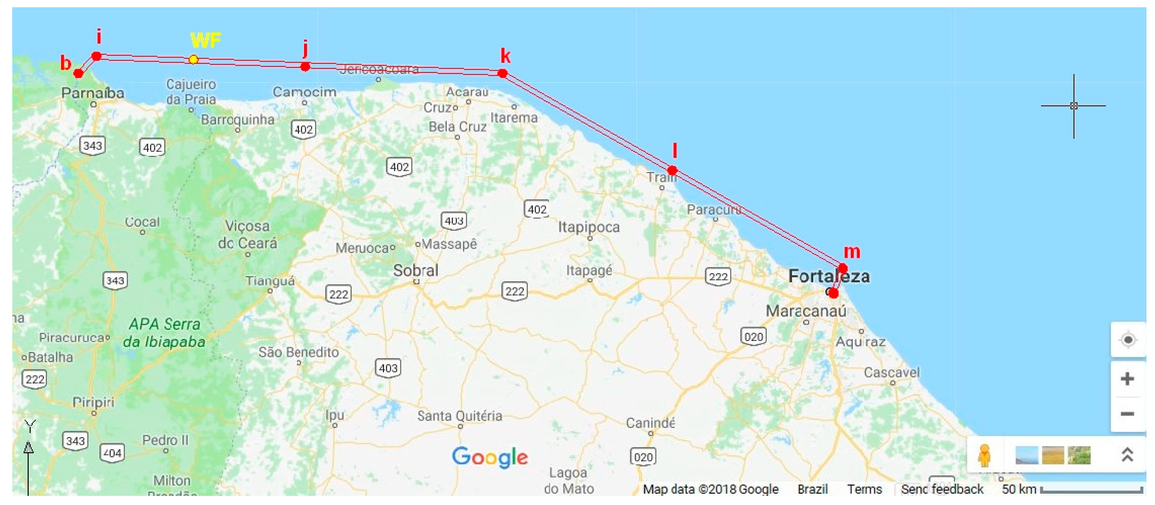
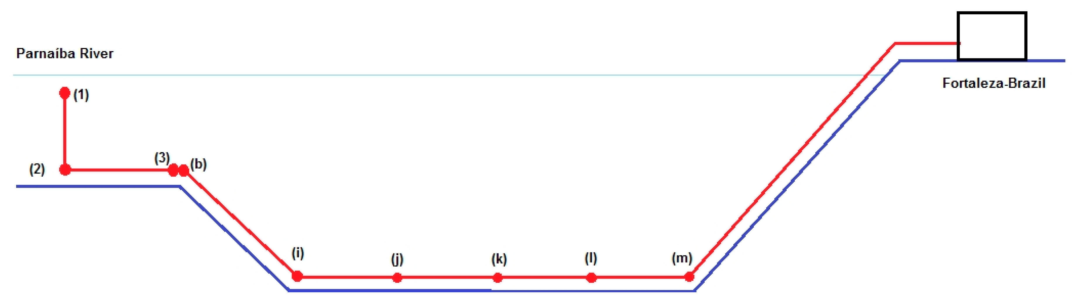
. Our results were estimates based on calculations according to the literature. The discharge line was almost all the same level and the electrical power supply was completely from wind power. The layout of the pipelines defined by Figure 11, Figure 12 and Figure 13 characterizes each system, depending on the water demand and selected rivers. The stretches of the route Parnaíba/Fortaleza were calculated and are represented in Figure 11, and its characterization is presented in Table 4 for Scenarios 1 and 2.

The diameter of the pipelines was found through the Bresse formula (Equation (1)), for the function of flow rate demanded for the metropolises. From this diameter, considering the speed flow and the length of the stretch, was found the overall head losses of each stretch through Equation (2).

The power of the hydraulic pump was found through Equation (7) considering a pump efficiency of 92% and the overall head losses. The electric power of the motor to drive the pump was given by Equation (12) in function of flow rate, discharge, pump efficiency, electrical efficiency, and mechanical efficiency.

In this project, we did not list the reservation delivery structures, distribution tank, Moorhen treatment systems and distribution network, which according to [1] are part of the water distribution system, as this study aimed to only technically and economically check the transportation of raw water.

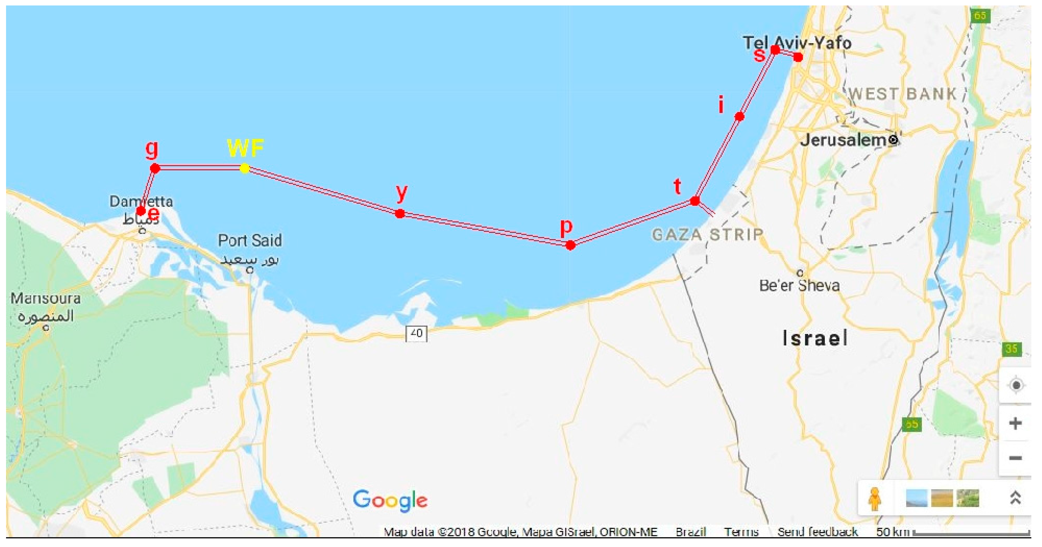
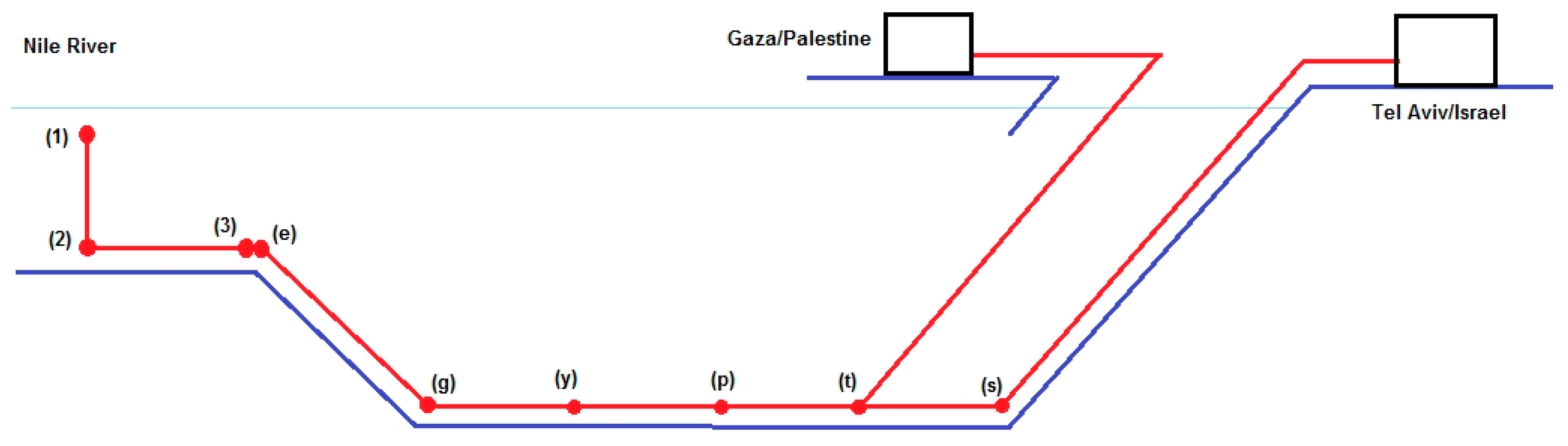
The stretches of the Nile route/Tel Aviv-Gaza are represented in Figure 12; the characterization of the sections of this route is shown in Table 5 for Scenarios 1 and 2.

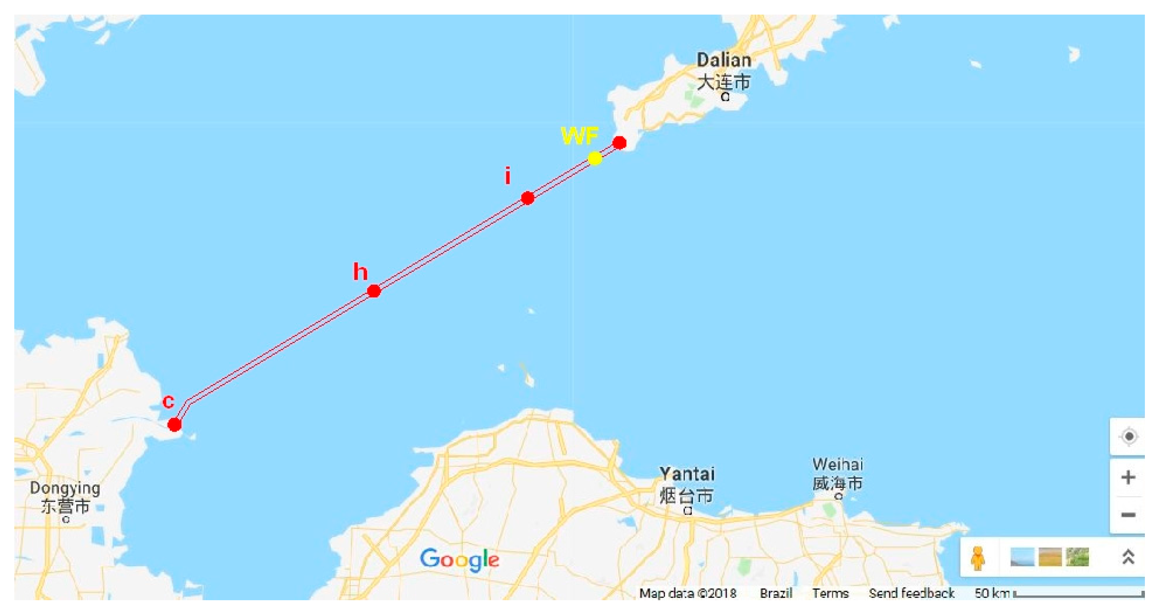
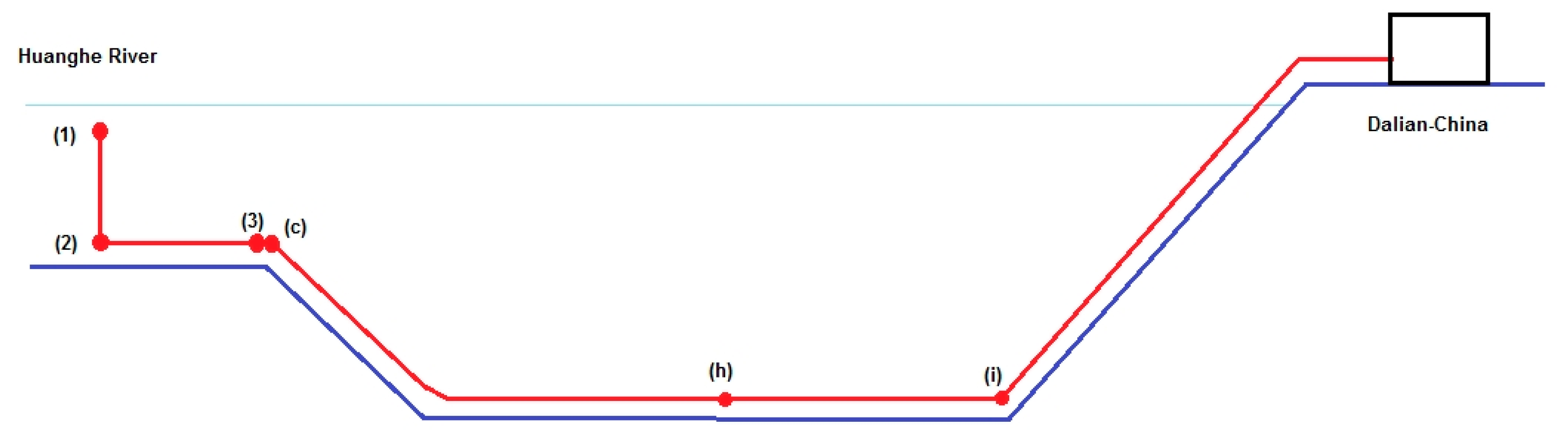
The stretches of the route of the Huanghe/Dalian-China is represented in Figure 13, the characterization of the sections of this route is shown in Table 6 for Scenarios 1 and 2.

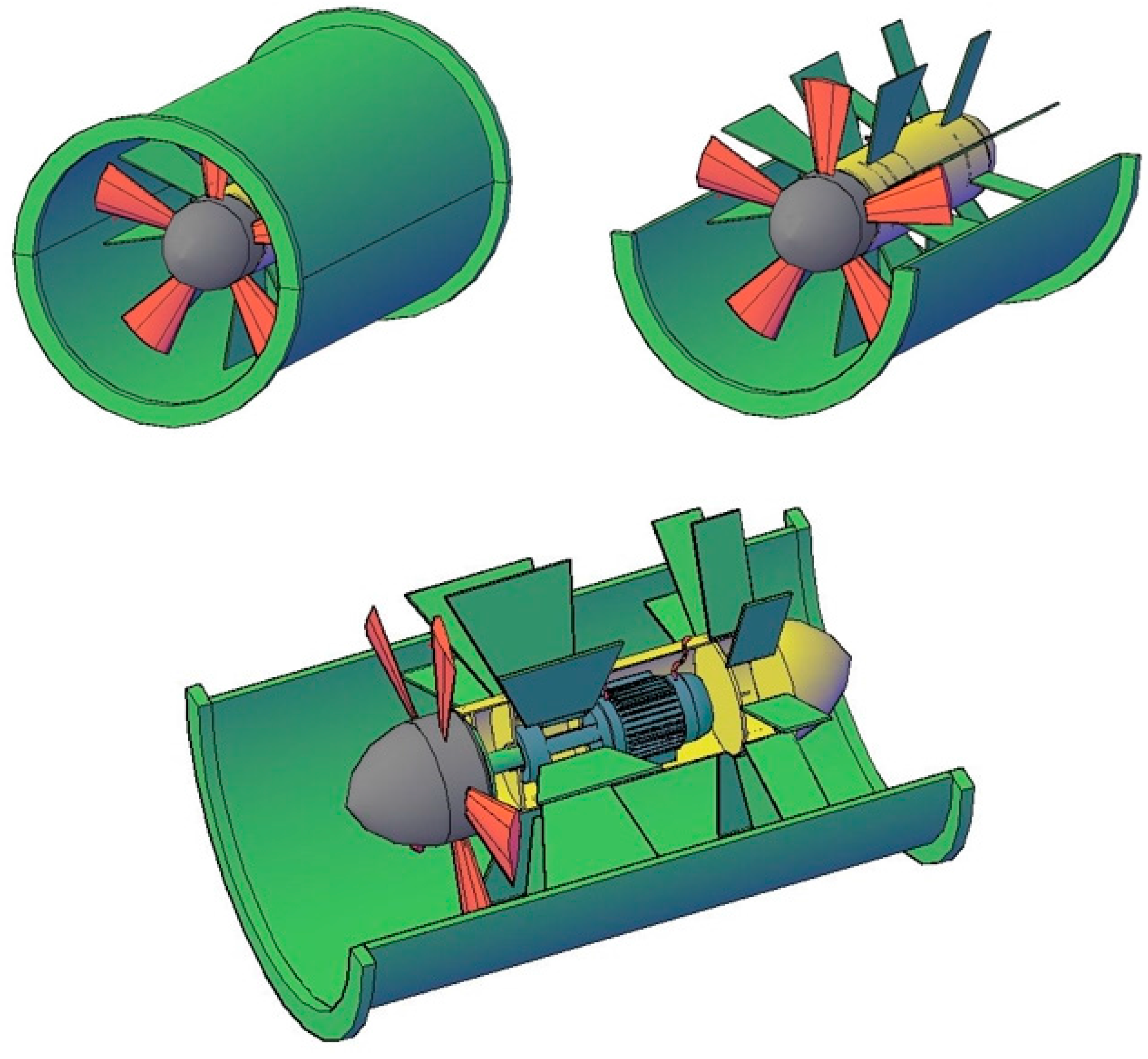
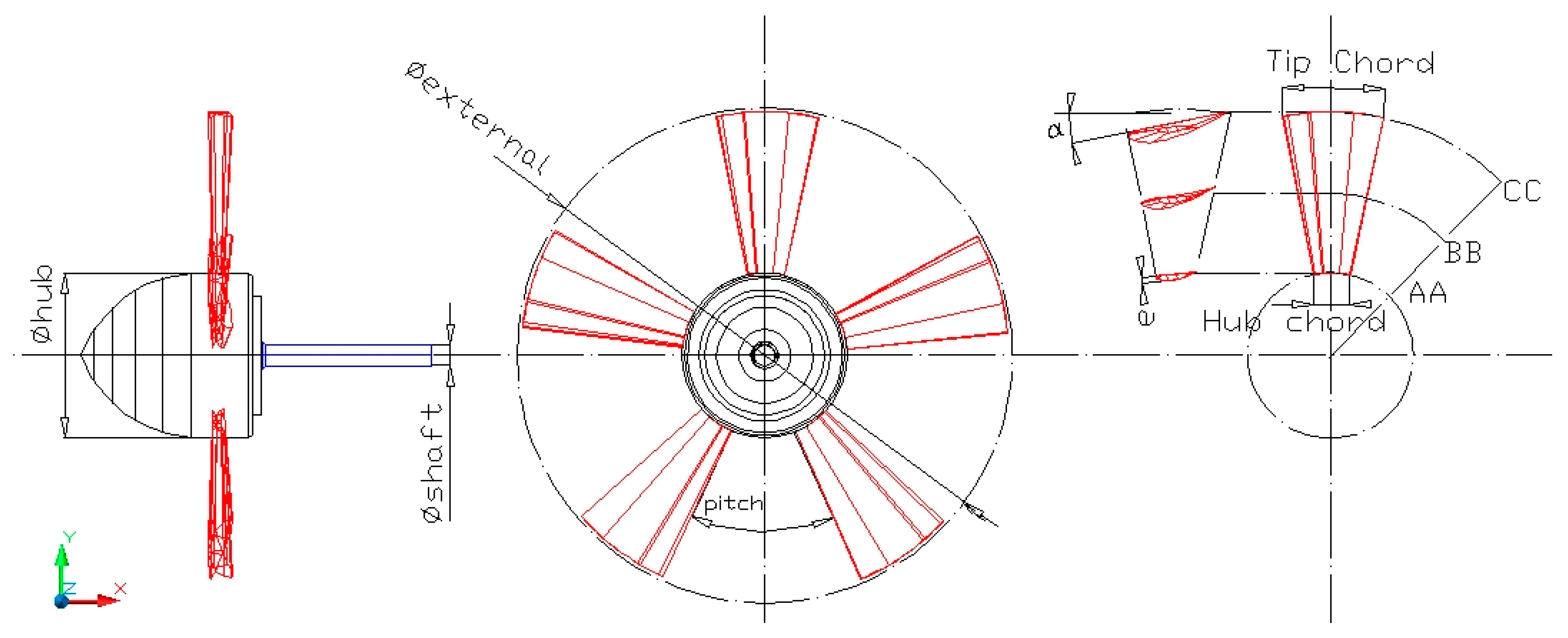
According to [1], when the water in the catchment has solids suspended with very high value, it is important to design a sand trap to settle these solids, thus avoiding their direct capture. Considering the characteristics of the Huanghe River in China, the construction is necessary to prevent damage to the pumping system. With a speed flow greater than the 0.6 m/s limit [63], there is no risk of deposition of sediment volumes along the pipe and maneuvering stations. From the definition of underwater pipes were calculated the axial hydraulic pumps that offer the energy of the water flow so that the flow is obtained in response to demand in the metropolises. The conceptual design of the axial pump is shown in Figure 14.

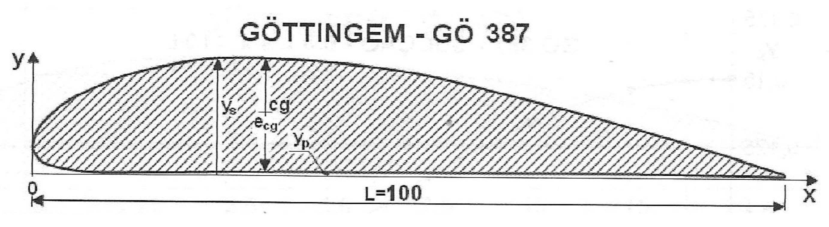
Considering the hydrofoil GO-387, the rotation of the hydraulic pump was found through Equation (8) as a function of the flow rate, the discharge, and the specific rotation obtained through Equation (9) that takes into account the suction height, water temperature, and the barometric height.

The pump rotor diameter was calculated by Equation (10), which relates the pump rotation (Equation (8)) and the tangential velocity of the flow. The hub diameter was calculated by Equation (11) as a function of the specific rotor rotation and pipeline diameter. The diameter of the drive shaft was given by Equation (13) as a function of the nominal motor power, safety factor, and shear stress of the chosen steel.

The number of blades of the pump rotor was calculated through Equation (14) as a function of the specific rotation of the rotor; the blade pitch was given by Equation (15); and the length of the hydrofoil rope by Equation (16) as a function of the relative flow velocity, relative flow angle, discharge, southern speed, and number of rotor blades. The angle of attack of the blade was given by Equation (17) as a function of the coefficient of support of the hydrofoil, the thickness of the hydrofoil, and the rope of the profile.

The design of the pumps is shown in

Table 7. Dimensions of the axial pumps for underwater pipelines Parnaíba/Fortaleza, Brazil. Scenario 1 (200 L/capita/day), Scenario 2 (81 L/capita/day).

SCENARIO 1
Pumping Station	External Diameter D (m)	Hub Diameter De (m)	Shaft Diameter d (m)	Pitch (m)	Tip Chord Lp (m)	Hub Chord Lc (m)	Hub Hydrofoil Thickness e (m)	Angle of Attack in Hub α (o)	Relative Angle in Hub β (o)	Blade Number	Rotation (RPM)
b	4.33	0.56	0.064	2.04	0.80	0.40	0.057	−10.6	18.8	2	248
i	4.33	1.23	0.096	1.70	0.50	0.25	0.036	−12.9	16.8	5	248
j	4.16	1.21	0.095	1.67	0.50	0.25	0.035	−13.0	16.4	5	259
k	3.99	1.18	0.094	1.63	0.49	0.24	0.035	−13.1	16.0	5	270
l	3.82	1.16	0.093	1.59	0.49	0.24	0.035	−13.2	15.6	5	281
m	3.66	1.20	0.130	1.63	0.54	0.27	0.038	−12.5	16.3	5	294
SCENARIO 2
Pumping Station	External Diameter D (m)	Hub Diameter De (m)	Shaft Diameter d (m)	Pitch (m)	Tip Chord Lp (m)	Hub Chord Lc (m)	Hub Hydrofoil Thickness e (m)	Angle of Attack in Hub α (o)	Relative Angle in Hub β (o)	Blade Number	Rotation (RPM)
b	2.74	1.17	0.05	1.22	0.41	0.20	0.02	−14.3	10.3	3	393
i	2.74	0.96	0.086	1.29	0.47	0.23	0.03	−12.5	13.5	5	393
j	2.63	0.93	0.086	1.25	0.46	0.23	0.03	−12.3	13.3	5	410
k	2.52	0.91	0.085	1.21	0.46	0.23	0.03	−12.1	13.1	5	427
l	2.42	0.89	0.084	1.17	0.46	0.23	0.03	−11.9	12.9	5	446
m	2.32	0.89	0.083	1.16	0.50	0.25	0.03	−11.2	13.5	5	465

,

Table 8. Dimensions of the axial pumps for underwater pipeline Nile-Tel Aviv/Gaza. Scenario 1 (200 L/capita/day), Scenario 2 (81 L/capita/day).

SCENARIO 1
Pumping Station	External Diameter D (m)	Hub Diameter De (m)	Shaft Diameter d (m)	Pitch (m)	Tip Chord Lp (m)	Hub Chord Lc (m)	Hub Hydrofoil Thickness e (m)	Angle of Attack in Hub α (o)	Relative Angle in Hub β (o)	Blade Number	Rotation (RPM)
e	5.23	1.63	0.068	2.56	0.72	0.36	0.051	−11.2	21.6	2	206
g	5.02	2.90	0.100	1.82	0.52	0.26	0.037	−12.1	18.5	5	215
y	4.81	2.85	0.099	1.79	0.52	0.26	0.037	−12.4	17.9	5	224
p	4.62	2.80	0.098	1.75	0.51	0.25	0.036	−12.7	17.4	5	234
t	4.43	2.74	0.179	1.72	0;50	0.25	0.036	−12.9	17.0	5	244
s	3.52	2.53	0.158	1.59	0.53	0.26	0.038	−12.5	15.9	5	307
SCENARIO 2
Pumping Station	External Diameter D (m)	Hub Diameter De (m)	Shaft Diameter d (m)	Pitch (m)	Tip Chord Lp (m)	Hub Chord Lc (m)	Hub Hydrofoil Thickness e (m)	Angle of Attack in Hub α (o)	Relative Angle in Hub β (o)	Blade Number	Rotation (RPM)
e	2.64	0.52	0.567	1.82	0.60	0.30	0.04	−18.34	21.60	3	408
g	2.64	0.94	0.087	1.25	0.46	0.23	0.038	−12.43	13.32	5	408
y	2.54	0.91	0.087	1.22	0.46	0.23	0.037	−12.24	13.14	5	425
p	2.43	0.89	0.086	1.18	0.46	0.23	0.031	−12.04	12.97	5	443
t	2.33	0.86	0.0855	1.14	0.46	0.23	0.031	−11.82	12.81	5	462
s	2.24	0.86	0.085	1.13	0.50	0.25	0.033	−11.07	13.37	5	482

and

Table 9. Dimensions of the axial pumps for underwater pipeline Huanghe/Dalian-China. Scenario 1 (200 L/capita/day), Scenario 2 (81 L/capita/day).

SCENARIO 1
Pumping Station	External Diameter D (m)	Hub Diameter De (m)	Shaft Diameter d (m)	Pitch (m)	Tip Chord Lp (m)	Hub Chord Lc (m)	Hub Hydrofoil Thickness e (m)	Angle of Attack in Hub α (o)	Relative Angle in Hub β (o)	Blade Number	Rotation (RPM)
c	4.83	3.19	0.108	2.00	0.60	0.30	0.043	−11.7	19.4	2	223
h	4.64	2.80	0.098	1.76	0.51	0.25	0.036	−12.7	17.5	5	232
i	4.45	2.75	0.156	1.72	0.51	0.25	0.036	−12.9	17.0	5	242
SCENARIO 2
Pumping Station	External Diameter D (m)	Hub Diameter De (m)	Shaft Diameter d (m)	Pitch (m)	Tip Chord Lp (m)	Hub Chord Lc (m)	Hub Hydrofoil Thickness e (m)	Angle of Attack in Hub α (o)	Relative Angle in Hub β (o)	Blade Number	Rotation (RPM)
c	3.08	1.03	0.087	1.39	0.46	0.23	0.033	−12.9	14.1	3	350
h	2.95	1.00	0.086	1.35	0.46	0.23	0.033	−12.8	13.8	5	365
i	2.83	0.98	0.085	1.32	0.46	0.23	0.033	−12.7	13.6	5	381

for both scenarios. The main dimensions are shown in Figure 15.

The preliminary hydrodynamic design of the rotors of the hydraulic pumps prescribed a special care with the cavitation phenomenon, which was reduced by the low-speed of the pumps at a low flow speed (0.88 m/s); however, even with these operating conditions, it is possible that cavitation occurs. This preliminary design of the axial rotor did not focus on the optimization of same, both in terms of cavitation as in efficiency. For the final design of the rotors, the top gap and the geometric design of the impellers—mainly in terms of displacement of the profiles in the region near the tip of the blade—need to be assessed, according to [64]. This optimization was outside the scope of this work but is necessary for obtaining the best efficiency of the pump.

Table 4, Table 5 and Table 6 show that the power of the electric motors needed to drive the pumps was high, so installation of such engines is not trivial in submerged water pumps, both in terms of cooling the engines as the structural seal as well as the axes. In this context, it evaluated the possibility of an electrical motor with a water-cooled system such as DC motors DCW [65], which are cooled by the heat exchanger air/water and reach up to 10 MW of power. According to [66], an estimate of the total cost of electric motors is US $ 110.00/kW. There are Chinese companies that specialize in pump submerged axial flows and since many products with very similar flow capacities to those required in this design are already on the market such as some commercial axial pump [67], it would be necessary to make adjustments to the designed rotor and the pump power required.

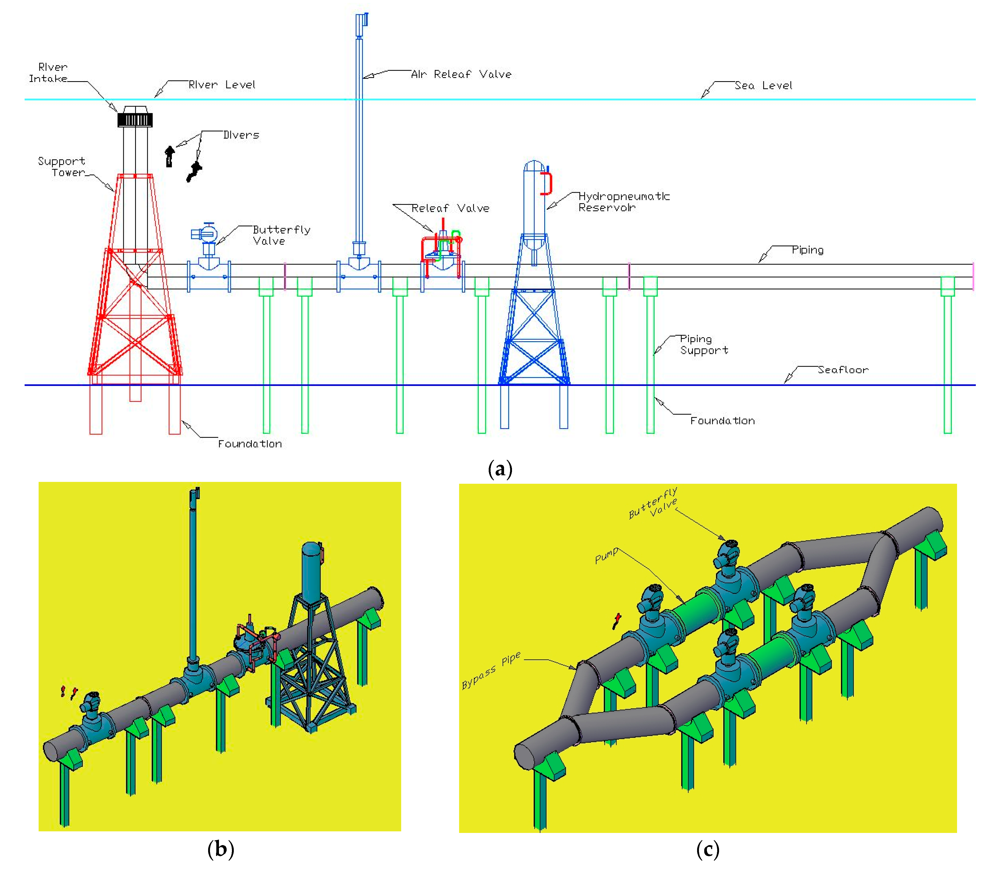
The conceptual design of stations of pipeline is shown in Figure 16.

The relief valve is integrated with a check valve to prevent in the event of an accident, there is a disastrous return of water flow. According to [68], it is a common practice in complex systems to improve reliability through systems and structures in standby (redundant) so that if one of the systems fail, the standby system takes action to avoid damage and loss to the end user. In this context, the pumping stations were equipped with two axial pumps, one in operation and one in standby, setting a redundant system. This configuration, though costly from the standpoint of equipment and structures, provides high reliability in underwater pipes.

The maintenance, repair, and replacement of the pumps will be undertaken by a system composed of trenchers machines and remoted operated vehicles (ROV) that specialize in the maintenance of submarine oil pipelines [69]. The pump lift and possible repairs will be carried out by an adapted wind turbine installation vessel [70].

All controls of the valves and pumps will be conducted by a modular electronics system via logical programmable controllers (PLC) that are combined in a control center to make real-time diagnostics of every pipeline.

The estimated dimensions show that it is a large system, with flows reaching tens of cubic meters per second. In such systems, special attention should be given to the hydraulic transients generated for the opening maneuvers, closing, or shunt [1]. In this context, the effects of water hammer were evaluated, which were calculated using Equation (6) as a function of flow speed and celerity (Equation (4)). The critical time for opening was found through Equation (5) as a function of celerity and pipe length. Based on this evaluation were the dimensioned armor and structural screens of reinforced concrete pipe and the security systems (relief valves and hydropneumatic tanks) as well as the maneuver times (closing and the opening of the butterfly valve or flow derivations). The focus was to avoid intense transient in this context for safety purposes, the pipe was dimensioned for the worst case scenario represented by a rapid maneuver, defined as the time where the maneuver was smaller than the critical time. The reinforced concrete pipe was coated externally with polyethylene. The strength of concrete was designed with a fck of 250 MPa and the reinforcing steel was the CA50 with fyk = 500 MPa. The thickness of the tube wall was standardized to 150 mm. With these determinations, it was possible to measure the area of the steel reinforcement and the area of the structural concrete, steel screen tube, which were calculated according to the method described by [71,72]. The resistance of the polyethylene layer was neglected. In the

Table 10. Characterization of hydraulic transients for pipeline Parnaíba/Fortaleza-Brazil. Scenario 1 (200 L/capita/day), Scenario 2 (81 L/capita/day).

SCENARIO 1
Stretch	Internal Diameter (m)	Stretch Length (m)	Effective Speed (m/s)	Overpressure Hydraulic Transient (m)	Critical Time (s)	Pipe Stress (MPa)	Area Stell Armor (m2)
Intake deep (2)	4.33	5	94.63	90.77	0.12	13.11	0.123
Free Run (2–3)	4.33	594	94.63	65.56	12.55	9.47	0.089
Station Pumping (b)	4.33	30,000	94.63	8.53	635.02	1.23	0.011
Station Pumping (i)	4.33	100,000	94.63	8.53	2113.42	1.23	0.011
Station Pumping (j)	4.15	100,000	96.61	8.71	2070.14	1.20	0.009
Station Pumping (k)	3.98	100,000	98.63	8.89	2027.61	1.18	0.008
Station Pumping (l)	3.82	100,000	100.72	9.08	1985.64	1.15	0.006
Station Pumping (m)	3.65	30,000	103.93	9.28	582.87	1.13	0.005
SCENARIO 2
Stretch	Internal Diameter (m)	Stretch Length (m)	Effective Speed (m/s)	Overpressure Hydraulic Transient (m)	Critical Time (s)	Pipe Stress (MPa)	Area Stell Armor (m2)
Intake deep (2)	2.74	5	118.94	114.09	0.08	10.40	0.0153
Free Run (2–3)	2.74	594	118.94	82.41	8.41	7.51	0.0110
Station Pumping (b)	2.74	30,000	118.94	10.73	5590.75	0.97	0.0014
Station Pumping (i)	2.74	100,000	118.94	10.72	18,641.74	0.97	0.0014
Station Pumping (j)	2.74	100,000	121.39	10.95	18,259.67	0.95	0.0011
Station Pumping (k)	2.63	100,000	123.93	11.18	17,885.53	0.93	0.0009
Station Pumping (l)	2.52	100,000	126.52	11.41	17,519.16	0.91	0.0008
Station Pumping (m)	2.42	30,000	129.17	11.65	5148.12	0.90	0.0006

,

Table 11. Characterization of hydraulic transients for pipeline Nile-Tel Aviv/Gaza. Scenario 1 (200 L/capita/day), Scenario 2 (81 L/capita/day).

SCENARIO 1
Stretch	Internal Diameter (m)	Stretch Length (m)	Effective Speed (m/s)	Overpressure Hydraulic Transient (m)	Critical Time (s)	Pipe Stress (MPa)	Area Stell Armor (m2)
Intake deep (2)	5.23	5	86.16	82.64	0.11	14.41	0.2908
Free Run (2–3)	5.23	739	86.16	59.69	17.16	10.40	0.2100
Station Pumping (e)	5.23	30,000	86.16	7.77	696.34	1.35	0.0273
Station Pumping (g)	5.01	100,000	87.97	7.93	2273.43	1.32	0.0226
Station Pumping (y)	4.81	100,000	89.82	8.10	2226.64	1.29	0.0187
Station Pumping (p)	4.61	100,000	91.69	8.27	2181.11	1.27	0.0155
Station Pumping (t)	4.42	100,000	93.63	8.44	2136.05	1.24	0.0128
Station Pumping (s)	3.51	30,000	104.99	9.47	571.46	1.11	0.0045
SCENARIO 2
Stretch	Internal Diameter (m)	Stretch Length (m)	Effective Speed (m/s)	Overpressure Hydraulic Transient (m)	Critical Time (s)	Pipe Stress (MPa)	Area Stell Armor (m2)
Intake deep (2)	2.64	5	121.02	116.08	0.16	10.22	0.0130
Free Run (2–3)	2.64	739	121.02	83.85	11.00	7.38	0.0094
Station Pumping (e)	2.64	30,000	121.02	10.91	991.55	0.96	0.0012
Station Pumping (g)	2.64	100,000	120.97	10.91	3306.49	0.96	0.0012
Station Pumping (y)	2.64	100,000	123.50	11.14	3238.74	0.94	0.0010
Station Pumping (p)	2.54	100,000	126.08	11.37	3172.39	0.92	0.0008
Station Pumping (t)	2.43	100,000	128.72	11.61	3107.42	0.90	0.0006
Station Pumping (s)	2.33	30,000	131.41	11.85	913.14	0.88	0.0005

and

Table 12. Characterization of hydraulic transients for pipeline Huanghe/Dalian-China. Scenario 1 (200 L/capita/day), Scenario 2 (81 L/capita/day).

SCENARIO 1
Stretch	Internal Diameter (m)	Stretch Length (m)	Effective Speed (m/s)	Overpressure Hydraulic Transient (m)	Critical Time (s)	Pipe Stress (MPa)	Area Stell Armor (m2)
Intake deep (2)	4.83	5	89.61	85.95	0.11	13.85	0.893
Free Run (2–3)	4.83	674	89.61	62.08	15.06	10.00	0.645
Station Pumping (c)	4.83	130,000	89.61	8.08	2901.34	1.30	0.084
Station Pumping (h)	4.63	100,000	91.48	8.25	2186.23	1.27	0.079
Station Pumping (i)	4.44	100,000	93.39	8.42	2141.50	1.24	0.074
SCENARIO 2
Stretch	Internal Diameter (m)	Stretch Length (m)	Effective Speed (m/s)	Overpressure Hydraulic Transient (m)	Critical Time (s)	Pipe Stress (MPa)	Area Stell Armor (m2)
Intake deep (2)	3.21	5	107.62	101.11	0.09	11.75	0.0460
Free Run (2–3)	3.21	674	109.88	74.57	11.77	8.31	0.0276
Station Pumping (c)	3.21	130,000	112.18	10.12	19,758.90	1.03	0.0024
Station Pumping (h)	3.08	100,000	114.53	10.33	19,353.64	1.01	0.0020
Station Pumping (i)	2.95	100,000	116.93	10.55	18,956.78	0.99	0.0016

show the values of the speed, hydraulic transients, critical maneuver times, the stresses applied to the tubes, the areas of the armor and the areas of steel screen per linear meter of pipe for each section of the route of the pipeline in each metropolis. All values had a safety factor of 2.

The pipe installation on the seabed will be undertaken by a specially adapted wind turbine installation vessel. According to [70], the time to install an offshore wind turbine can reach 18 h, and by [73], the cost of installation of the foundation of one offshore turbine is US $ 290,000.00, therefore one hour of work costs around US $ 16,439.00. Whereas it is much simpler to install a concrete pipe on the seabed, which can be used as basis of the pipe laying vessel [74] with an estimated rate of installation of 140 m/h (around a third of rate of the PLV ship), so for the installation of 1 km, 7.14 h is needed, so it has an estimated cost of US $ 115,000.00/km for the pipe installation.

With the setup of the defining pipeline and their paths completed, it was possible to allocate the wind farms and to scale them. For security, the wind farms will be available in addition to the required turbines, with two more turbines: one for emergency backup purposes [68], and the other for the maintenance schedule [57], so that there will always be an operational turbine on standby and the other in maintenance. The preliminary design of the wind farms is presented in

Table 13. Dimensioning of Wind Farms for pipelines. Scenario 1 (200 L/capita/day).

Fortaleza/Parnaíba
Season	Wind Speed at 10 m (m/s)	Wind Speed at 130 m (m/s)	Electric Motor Power—Total (MW)	Wind Turbine Number ** (Unit)	Wind Turbine Power—Total (MW)	Power—Reserve (MW)
Winter	10	16.9	11.0	4	12.0	1.0
Spring	9.5	16.0	11.0	4	12.0	1.0
Summer	7.5	12.7	11.0	4	12.0	1.0
Autumn	7.5	12.7	11.0	4	12.0	1.0
Yearly Total	-	-	44.0	-	48.0	4.0
Tel Avivi-Gaza/Nile
Season	Wind Speed at 10 m (m/s)	Wind Speed at 130 m (m/s)	Electric Motor Power—Total (MW)	Wind Turbine Number ** (Unit)	Wind Turbine Power—Total (MW)	Power—Reserve (MW)
Winter	3.5	6.3	24.12	23	16.10	−8.02
Spring	5.0	9.0	24.12	23	40.25	16.13
Summer	5.0	9.0	24.12	23	40.25	16.13
Autumn	2.5	4.5	24.12	23	0.00	−24.12
Yearly Total	-	-	96.48	-	96.60	0.12
Dalian/Huanghe
Season	Wind Speed at 10 m (m/s)	Wind Speed at 130 m (m/s)	Electric Motor Power—Total (MW)	Wind Turbine Number ** (Unit)	Wind Turbine Power—Total (MW)	Power—Reserve (MW)
Winter	4.5	8.1	11.32	19	26.60	15.27
Spring	2,5	4.5	11.32	19	0.00	−11.32
Summer	4.5	8.1	11.32	19	26.60	15.27
Autumn	2.0	3.6	11.35	19	0.00	−11.32
Yearly Total			45.28	-	53.20	7.92

Note: ** Excluding standby turbine and turbine in maintenance.

and

Table 14. Dimensioning of Wind Farms for pipelines. Scenario 2 (81 L/capita/day).

Fortaleza/Parnaíba
Season	Wind Speed at 10 m (m/s)	Wind Speed at 130 m (m/s)	Electric Motor Power—Total (MW)	Wind Turbine Number ** (Unit)	Wind Turbine Power—Total (MW)	Power—Reserve (MW)
Winter	10	16.9	5.77	3	9.0	3.23
Spring	9.5	16.0	5.77	3	9.0	3.23
Summer	7.5	12.7	5.77	3	9.0	3.23
Autumn	7.5	12.7	5.77	3	9.0	3.23
Yearly Total	-	-	23.08	-	36.0	12.92
Tel Avivi-Gaza/Nile
Season	Wind Speed at 10 m (m/s)	Wind Speed at 130 m (m/s)	Electric Motor Power—Total (MW)	Wind Turbine Number ** (Unit)	Wind Turbine Power—Total (MW)	Power—Reserve (MW)
Winter	3.5	6.3	5.60	8	4.90	−0.70
Spring	5.0	9.0	5.60	8	14.00	8.39
Summer	5.0	9.0	5.60	8	14.00	8.39
Autumn	2.5	4.5	5.60	8	0.00	−5.60
Yearly Total	-	-	22.40	-	96.60	3.46
Dalian/Huanghe
Season	Wind Speed at 10 m (m/s)	Wind Speed at 130 m (m/s)	Electric Motor Power—Total (MW)	Wind Turbine Number ** (Unit)	Wind Turbine Power—Total (MW)	Power—Reserve (MW)
Winter	4.5	8.1	4.03	7	9.80	5.76
Spring	2.5	4,5	4.03	7	0.00	−11.32
Summer	4.5	8.1	4.03	7	9.80	5.76
Autumn	2.0	3.6	4.03	7	0.00	−11.32
Yearly Total			16.14	-	19.60	3.48

Note: ** Excluding standby turbine and turbine in maintenance.

.

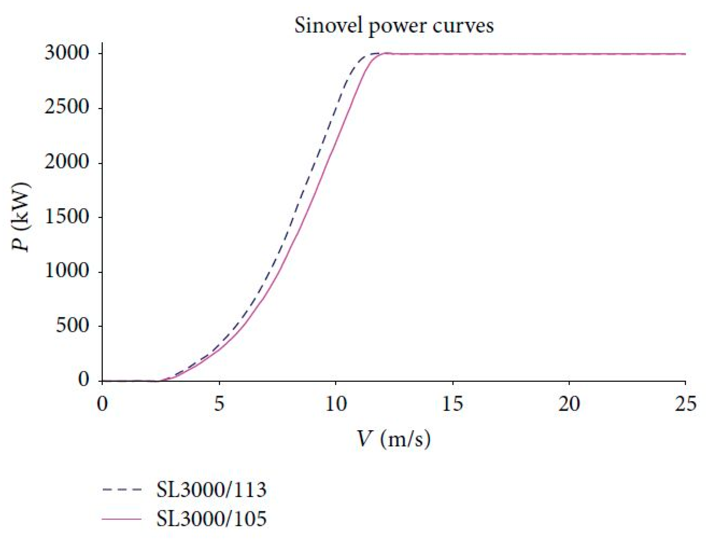
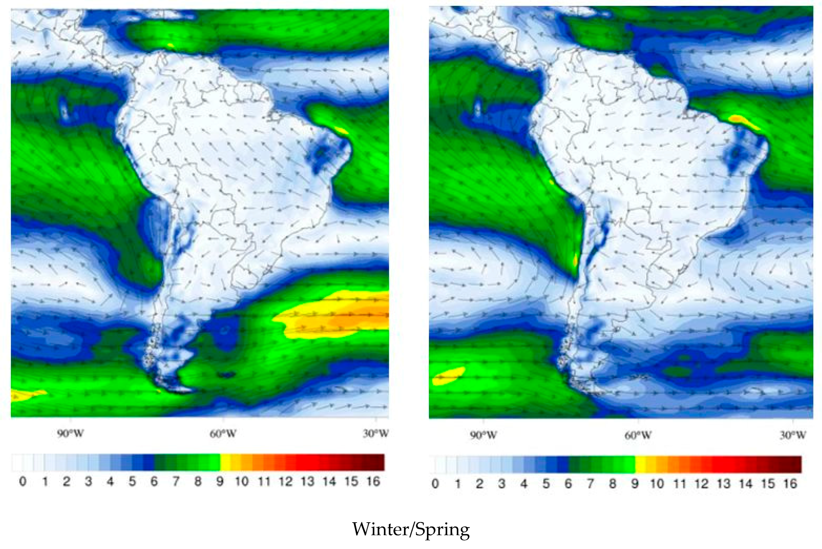
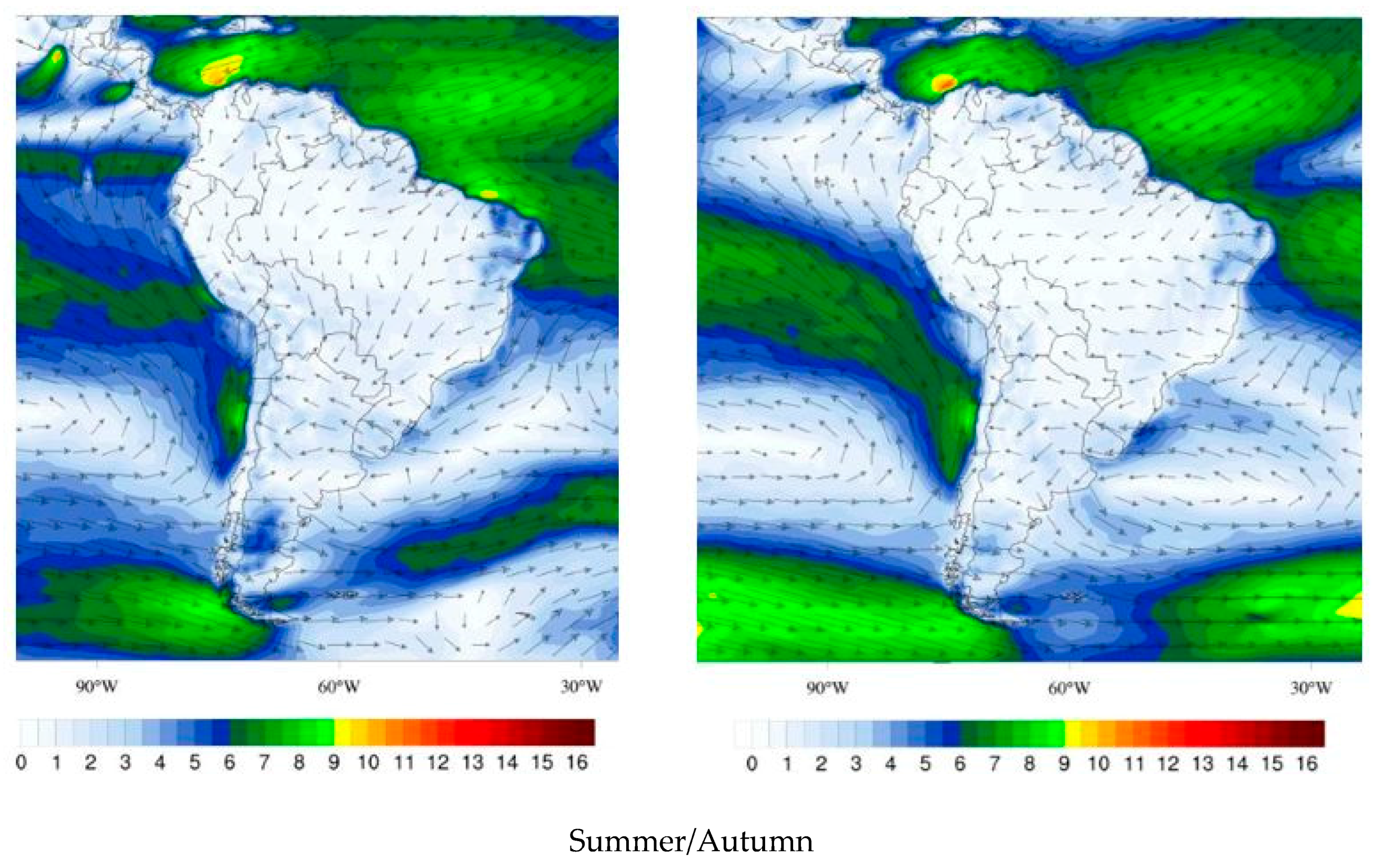
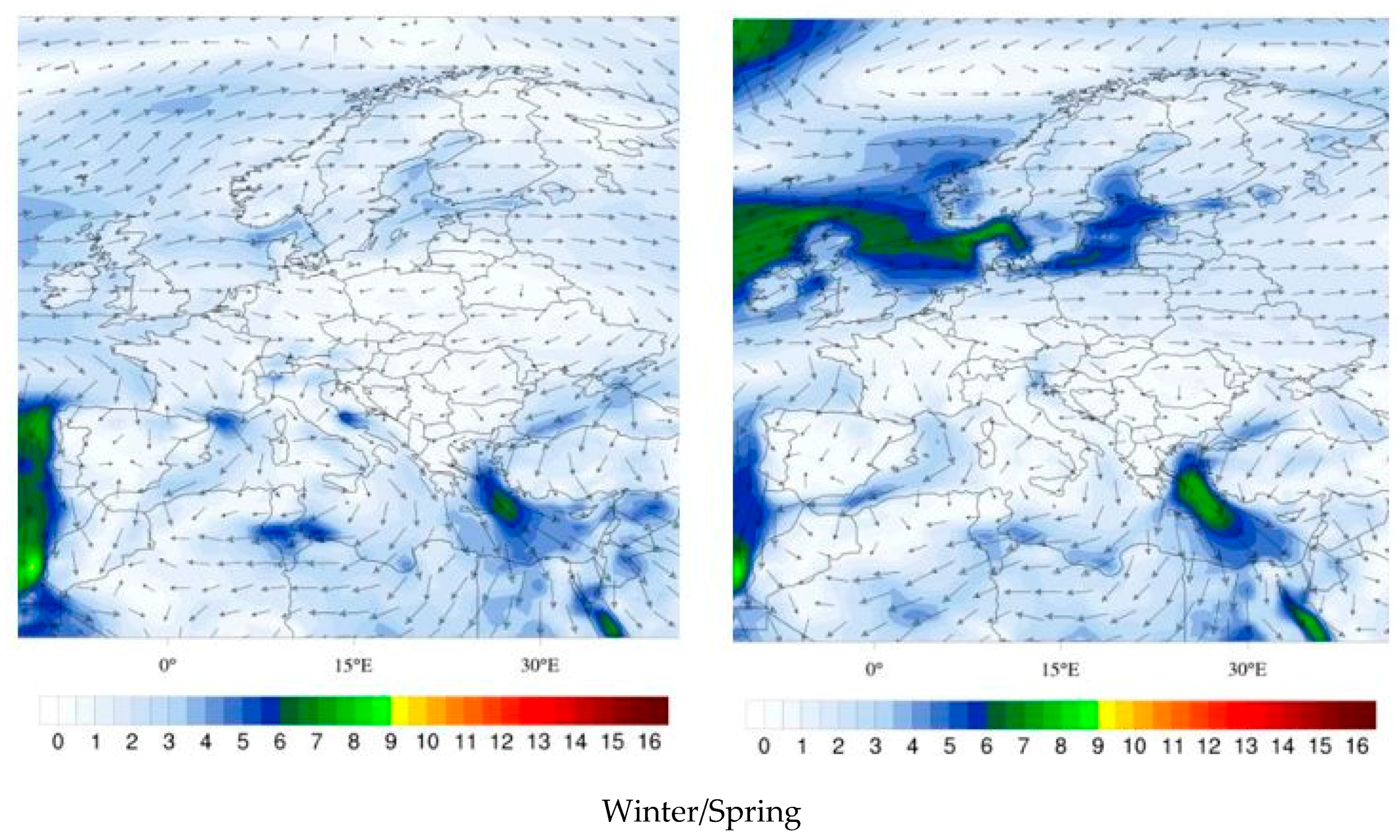
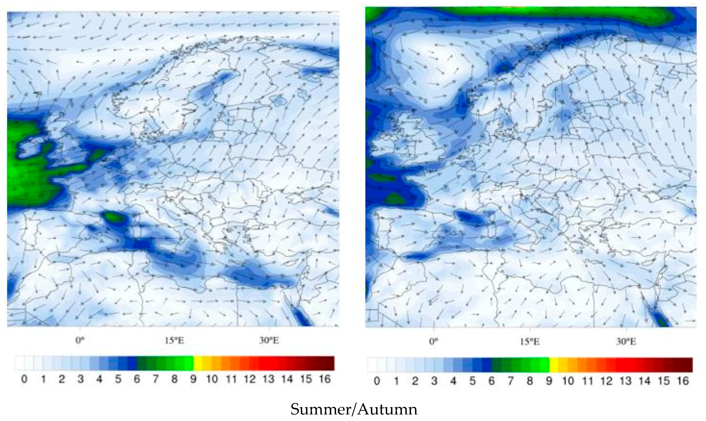
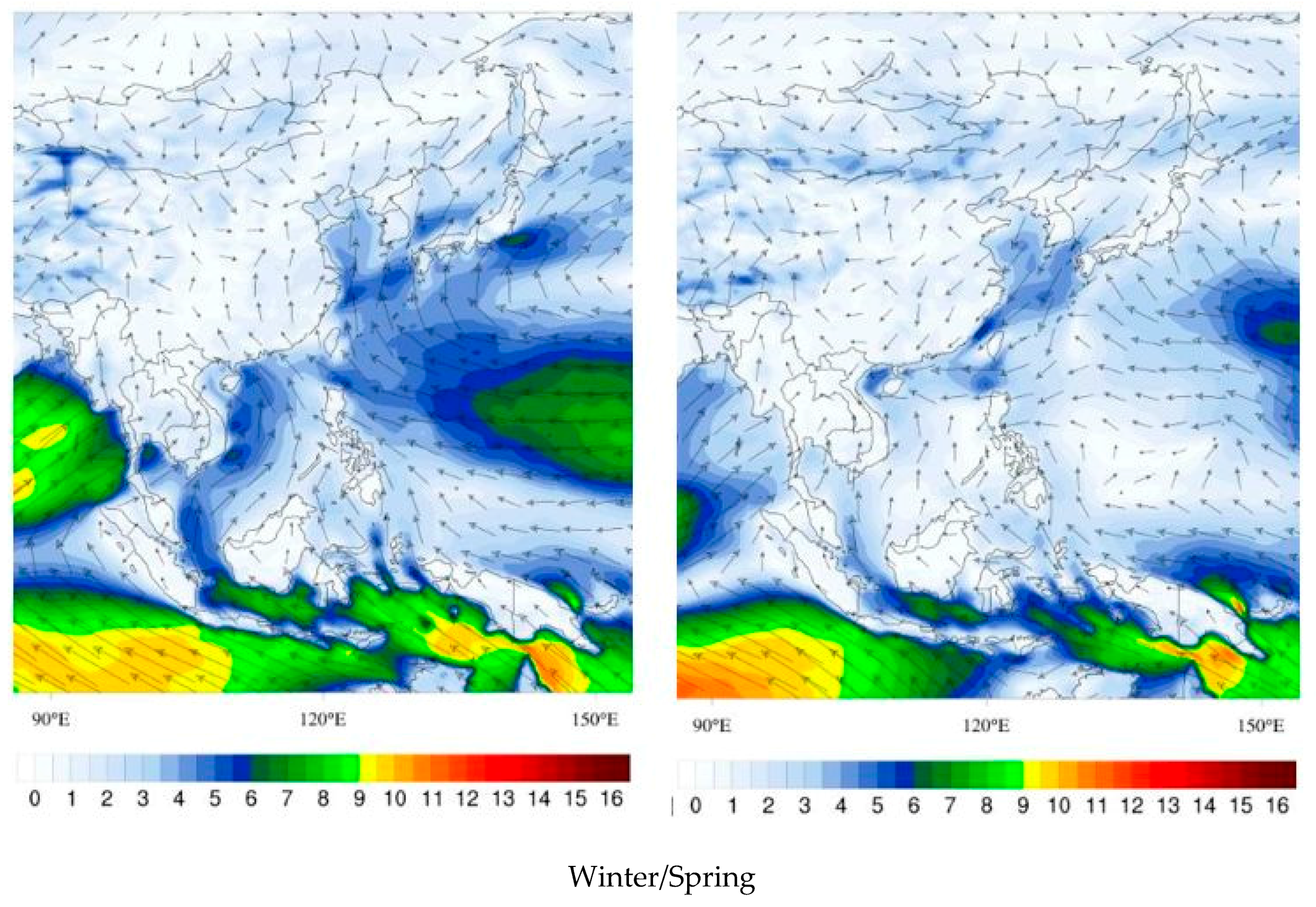
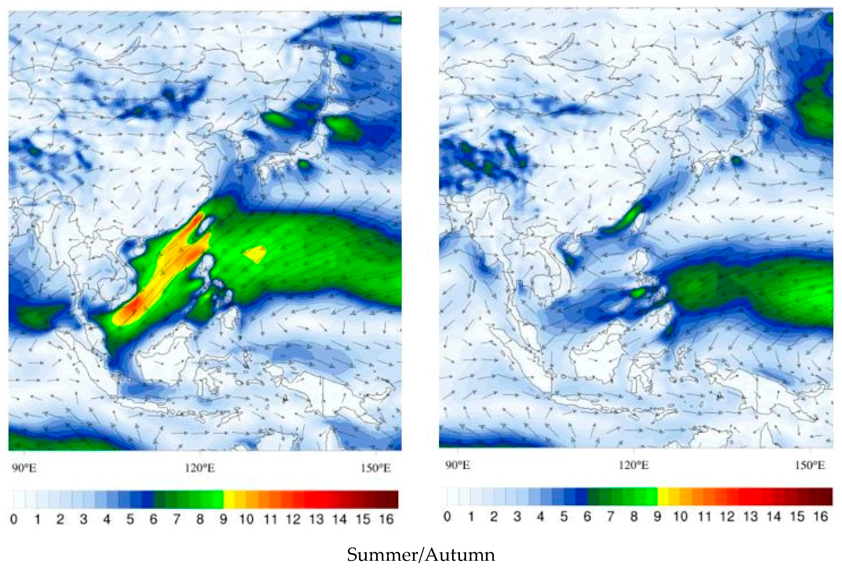
The power curve of the wind turbine offshore Sinovel SL3000-113 is shown in Figure 10 [59], the location of the wind farms in the path of the pipelines is shown in Figure 2, Figure 3 and Figure 4; the wind maps in each coverage area of the metropolis are shown in Figure 5, Figure 6 and Figure 7. The preliminary design of the wind farms is presented in the following tables:

For the power demand of the electric motors and the total generation of wind farms is perceived that only Pipeline Parnaíba/Fortaleza, Brazil had an independent operating capacity without a link to the mainland electricity distribution network, as in all seasons there was a net power reserve as the Brazilian northeastern coast winds are intense all year.

For the system of the Nile/Tel Aviv-Gaza and Huanghe/Dalian, there were deficits in several seasons, this required a connection to the mainland grid electricity distribution to meet the demand of the electric motors when the wind regime was not able to trigger the wind turbines.

According to [75], the energy cost, operational cost, maintenance cost, and capital investment were the main contributors to the water production cost. The energy cost is responsible for about 50% of the produced water cost. In this context, it is clear that with the use of offshore wind energy, the cost of raw water transport can be reduced by half, indicating the great feasibility of using offshore wind turbines, even considering that wind farms in China and Egypt will have long periods of inactivity due to low winds.

However, if the excess energy of the wind periods in the continental power grid could be shed, it is possible to compensate for periods without wind using the continental electrical power, thus making the system viable energetically. Currently in Brazil, companies can release the excess energy of an independent power generation system in the utility distribution network, earning credits for later use [76]. This fact enables Brazilian wind farms to throw their surplus power to the grid, which in addition to the energy-sustaining underwater pipe also generates income. In assessing Table 13 and Table 14, it can be deduced that there is a significant annual net energy reserve in Chinese wind farms and although there are seasons without wind, the wind energy in seasons where there is electrical power generation is higher than the demand for electric motors, which compensates for windless seasons. If by chance there is a distributed generation policy similar to that of Brazil, this would completely allow the Chinese wind farms making the Huanghe/Dalian system to have sustainable energy.

The wind farms of the Nile/Tel Aviv-Gaza system, the net reserve was small, but still, the argument is similar to the distributed generation case for Huanghe/Dalian. With all sizing and definitions of elements and systems of underwater pipes, it was possible to estimate the budget as well as the assessment of the investment. The following tables show the estimated budget for each pipeline.

Table 15. Estimated Cost of Investment for pipelines-Scenario 1 (200 L/capita/day).

Parnaíba/Fortaleza, Brazil
Cost Element	Unit	Amount	Unit Value (US $)	Total Value (US $)	Source
Hydraulic pumps	pump	12	80,000.00	960,000.00	(1)
Electric Motor	MW	11	110,000.00	1,210,000.00	(16)
Wind turbines (turbine + foundation + installation)	turbine	6	1,403,428.00	8,420,568.00	(2)
Reinforced concrete pipe	meter	460,000	289.14	133,004,400.00	(3), (4)
Installation of pipeline in seabed	kilometer	460	115,000.00	52,900,000.00	(13),(14),(15)
Relief valve	Valve	30	15,274.00	458,220.00	(5)
Air relief valve	Valve	30	2000.00	60,000.00	(6)
Butterfly valve	Valve	30	20,000.00	600,000.00	(7)
Hydropneumatic reservoir	Reservoir	30	30,000.00	900,000.00	(8)
Transmission system power	Full system	1	-	36,665,220.00	(9)
Submerged concrete foundations	Cubic meter	12.137	288.85	3,505,788.80	(10)
Submerged concrete support structures, anchor, engineering structures	units	46,000	100.57	10,177,684.00	(10)
Submerged tower	units	4	102,300.00	409,200.00	(12)
TOTAL INVESTIMENT	-	-		249,271,081.00
Cost of annual O&M	year	30	415,451.80	-	(11)
Nile-Tel Aviv/Gaza
Cost Element	Unit	Amount	Unit Value (US $)	Total Value (US $)	Source
Hydraulic pumps	pump	12	80,000.00	960,000.00	(1)
Electric Motor	MW	24.12	110,000.00	2,653,200.00	(16)
Wind turbines (turbine + foundation + installation)	turbine	25	1,403,428.00	35,085,700.00	(2)
Reinforced concrete pipe	meter	460,000	289.14	133,004,400.00	(3), (4)
Installation of pipeline in seabed	kilometer	460	115,000.00	52,900,000.00	(13),(14),(15)
Relief valve	Valve	36	15,274.00	549,864.00	(5)
Air relief valve	Valve	36	2000.00	72,000.00	(6)
Butterfly valve	Valve	36	20,000.00	720,000.00	(7)
Hydropneumatic reservoir	Reservoir	36	30,000.00	1,080,000.00	(8)
Transmission system power	Full system	1	-	36,665,220.00	(9)
Submerged concrete foundations	Cubic meter	12,137	288.85	3,505,788.80	(10)
Submerged concrete support structures, anchor, engineering structures	units	46,000	100.57	10,177,684.00	(10)
Submerged tower	units	6	102,300.00	613,800.00	(12)
TOTAL INVESTIMENT	-	-		277,987,656.80
Cost of annual O&M	year	30	463,312.76	-	(11)
Huanghe/Dalian-China
Cost Element	Unit	Amount	Unit Value (US $)	Total Value (US $)	Source
Hydraulic pumps	pump	8	80,000.00	640,000.00	(1)
Electric Motor	MW	11.32	110,000.00	1,245,200.00	(16)
Wind turbines (turbine + foundation + installation)	turbine	21	1,403,428.00	29,471,988.00	(2)
Reinforced concrete pipe	meter	330.000	289.14	95,416,200.00	(3), (4)
Installation of pipeline in seabed	kilometer	330	115,000.00	37,950,000.00	(13),(14),(15)
Releaf valve	Valve	22	15,274.00	336,028.00	(5)
Air releaf valve	Valve	22	2000.00	44,000.00	(6)
Buttefly valve	Valve	22	20,000.00	440,000.00	(7)
Hydropneumatic reservoir	Reservoir	22	30,000.00	660,000.00	(8)
Transmission system power	Full system		-	36,665,220.00	(9)
Submerged concrete foundations	Cubic meter	8.707	288.85	2,515,022.00	(10)
Submerged concrete support structures, anchor, engineering structures	units	33.000	100.57	7,301,382.00	(10)
Submerged tower	units	4	102,300.00	409,200.00	(12)
TOTAL INVESTIMENT	-		-	213,094,240.00
Cost of annual O&M	year	30	355,157.10	-	(11)

Source: (1) [68]; (2) [76]; (3) [77]; (4) [78]; (5) [79]; (6) [80]; (7) [81]; (8) [82]; (9) [83]; (10) [84]; (12) [85]; (12) [86], (13) [73], (14) [70], (15) [74]; (16) [66].

and

Table 16. Estimated Cost of Investment for pipelines-Scenario 2 (81 L/capita/day).

Parnaíba/Fortaleza, Brazil
Cost Element	Unit	Amount	Unit Value (US $)	Total Value (US $)	Source
Hydraulic pumps	pump	12	80,000.00	960,000.00	(1)
Electric Motor	MW	5.77	110,000.00	634,700.00	(16)
Wind turbines (turbine + foundation + installation)	turbine	5	1,403,428.00	7,017,140.00	(2)
Reinforced concrete pipe	meter	460,000	178.68	82,192,800.00	(3), (4)
Installation of pipeline in seabed	kilometer	460	115,000.00	52,900,000.00	(13),(14),(15)
Relief valve	Valve	30	15,274.00	458,220.00	(5)
Air relief valve	Valve	30	2000.00	60,000.00	(6)
Butterfly valve	Valve	30	20,000.00	600,000.00	(7)
Hydropneumatic reservoir	Reservoir	30	30,000.00	900,000.00	(8)
Transmission system power	Full system	1	-	36,665,220.00	(9)
Submerged concrete foundations	Cubic meter	12.137	288.85	3,505,788.80	(10)
Submerged concrete support structures, anchor, engineering structures	units	46,000	100.57	10,177,684.00	(10)
Submerged tower	units	4	102,300.00	409,200.00	(12)
TOTAL INVESTIMENT	-	-		196,480,743.00
Cost of annual O&M	year	30	327,467.92	-	(11)
Nile-Tel Aviv/Gaza
Cost Element	Unit	Amount	Unit Value (US $)	Total Value (US $)	Source
Hydraulic pumps	pump	12	80,000.00	960,000.00	(1)
Electric Motor	MW	5.60	110,000.00	616,000.00	(16)
Wind turbines (turbine + foundation + installation)	turbine	7	1,403,428.00	9,823,996.00	(2)
Reinforced concrete pipe	meter	460,000	172.20	79,212,000.00	(3), (4)
Installation of pipeline in seabed	kilometer	460	115,000.00	52,900,000.00	(13),(14),(15)
Relief valve	Valve	36	15,274.00	549,864.00	(5)
Air relief valve	Valve	36	2000.00	72,000.00	(6)
Butterfly valve	Valve	36	20,000.00	720,000.00	(7)
Hydropneumatic reservoir	Reservoir	36	30,000.00	1,080,000.00	(8)
Transmission system power	Full system	1	-	36,665,220.00	(9)
Submerged concrete foundations	Cubic meter	12,137	288.85	3,505,788.80	(10)
Submerged concrete support structures, anchor, engineering structures	units	46,000	100.57	10,177,684.00	(10)
Submerged tower	units	6	102,300.00	613,800.00	(12)
TOTAL INVESTIMENT	-	-		196,896,352.00
Cost of annual O&M	year	30	328,160.59	-	(11)
Huanghe/Dalian-China
Cost Element	Unit	Amount	Unit Value (US $)	Total Value (US $)	Source
Hydraulic pumps	pump	8	80,000.00	640,000.00	(1)
Electric Motor	MW	4.03	110,000.00	443,300.00	(16)
Wind turbines (turbine + foundation + installation)	turbine	7	1,403,428.00	9,823,996.00	(2)
Reinforced concrete pipe	meter	330.000	161.20	53,196,000.00	(3), (4)
Installation of pipeline in seabed	kilometer	330	115,000.00	37,950,000.00	(13),(14),(15)
Relief valve	Valve	22	15,274.00	336,028.00	(5)
Air relief valve	Valve	22	2000.00	44,000.00	(6)
Butterfly valve	Valve	22	20,000.00	440,000.00	(7)
Hydropneumatic reservoir	Reservoir	22	30,000.00	660,000.00	(8)
Transmission system power	Full system		-	36,665,220.00	(9)
Submerged concrete foundations	Cubic meter	8.707	288.85	2,515,022.00	(10)
Submerged concrete support structures, anchor, engineering structures	units	33.000	100.57	7,301,382.00	(10)
Submerged tower	units	4	102,300.00	409,200.00	(12)
TOTAL INVESTIMENT	-		-	150,424,148.00
Cost of annual O&M	year	30	250,706.91	-	(11)

Source: (1) [68]; (2) [76]; (3) [77]; (4) [78]; (5) [79]; (6) [80]; (7) [81]; (8) [82]; (9) [83]; (10) [84]; (12) [85]; (12) [86], (13) [73], (14) [70], (15) [74]; (16) [66].

are the estimated budget for each pipeline (scenario 1 and 2).

The estimated cost of investment to the order of US $ 250 million is very good since the value to construct the Anamurium Plant, which has a very close design to this proposal, was made with US $ 400 million [25]. In the Turkish-Cypriot system, although the pipeline’s total extension was only 106 km, the declared value of US $ 400 million included constructing a large dam with an estimated cost of US $ 330 million [86], therefore the pipeline itself was estimated at US $ 70 million.

With the values of the investment costs for the underwater pipes and the annual cost of maintenance, is was possible to make an economic analysis of the investment. The hurdle rate was set to 10.4%, the rate used by [62]. The value of raw water per cubic meter delivered in large cities was: Fortaleza-CE-Brazil = US $ 0.0355 [87]; Tel Aviv-Israel = US $ 0.3500 [88]; Dalian-China = US $ 0.0790 [89]. Depreciation was considered to be 3.3%, which represented the full value of the investment at the end of useful life.

The Present Worth Value was calculated by Equation (19) in terms of useful life, minimum internal rate return, cash flow, and capital investment. The Internal Rate of Return was calculated by Equation (20) in function of the disbursements, the investment time, the useful life. The payback was calculated by Equation (21) as a function of revenue at time, cost at time, and capital investment.

Table 17. Economic Analysis for underwater adductors.

Pipeline	Investment Cost (US $)	Annual Cost of Maintenance (US $)	Useful Life (Year)	Annual Water Demand (m3)	Raw Water Value (US $)	Depreciation Annual (US $)	Minimum Attractive Rate Return (%)	Internal Rate of Return (%)	Present Worth Value (US $)	Payback (Year)
Parnaíba/Fortaleza-Scenariao 1	249,271,081.00	415,451.80	30	293,284,800	10,429,207.49	8,309,036.00	10.4	-	−233,722,002.00	-
Parnaíba/Fortaleza-Scenariao 2	196,480,743.00	327,467.92	30	117,629,280	4,182,897,19	6,974,824.40	10.4	-	−221,052,603.32	-
Nile/Tel Aviv-Gaza-Scenario 1	277,987,656.80	463,312.76	30	405,868,320	142,053,912.00	9,266,255.00	10.4	47.60	928,968,361.13	2.10
Nile/Tel Aviv-Gaza-Scenario 2	196,896,352.00	328,160.59	30	109,745,280	38,410,848.00	6,563,211.73	10.4	9.67	16,380,136.50	9.69
Huanghe/Dalian-Scenario 1	213,094,240.00	355,157.10	30	433,620,000	34,255,980.00	7,103,141.00	10.4	12.17	31,332,613.16	7.95
Huanghe/Dalian-Scenario 2	150,424,148.00	250,706.91	30	175,655,520	13,876,786.08	5,104,138.26	10.4	3.91	71,872,964.52	17.46

presents an economic simulation of such a hypothesis, considering the hurdle rate of 10.4% [62].

Considering the scenario (200 L/capita/day), in the case of the Parnaíba/Fortaleza system, it had sufficient water availability and the wind conditions for wind power are ideal, but due to the low value of raw water per cubic meter (US $ 0.0355) there is no economic viability. It is interesting to note that this value is fixed by the State Government of Ceará by decree [87], requiring the Company of Water Resources Management to adopt this value regardless of the operation and climatic conditions of the region. Obviously, this very low value is not motivated by the “technical”, cost component, but certainly, there is a political consideration, as described by [22,90].

A second hypothesis for an underwater pipeline to Fortaleza would be the use of the excellent wind conditions of the region to install, in addition to the wind turbines required for the supply of energy to electric motors (6 turbines), another (34 turbines) for the sole purpose of generating electricity and launched in mainland network, thus producing dividends given that the value of MWh in Brazil for wind energy is around US $ 38.85 [91]. In this situation,

Table 18. Economic Simulation in hypothesis of systems coupled between raw water transport and wind power generation to Fortaleza.

Pipeline	Investment Cost (US $)	Annual Cost of Maintenance (US $)	Useful Life (Year)	Annual Water Demand (m3)	Raw Water Value (US $)	Wind Energy Value (US $)	Depreciation Annual (US $)	Internal Rate of Return (%)	Present Worth Value (US $)	Payback (Year)
Fortaleza	296,987,632.80	494,979.38	30	293,284,800	10,429,207.49	22,806,034.30	9,899,587.76	11.34	23,117,599.99	8.46

show that there is U$S 33,229,022.90 of dividends that makes the project feasible.

It can be argued that this assumption changes the core business, instead of being the raw water supply, it would become the generation of electricity. However, this solution would impact greatly on the welfare of the population, and also increase the volume of existing drinking water in Fortaleza currently, thus forming a reserve for possible drought, or use for trade and industry.

Another component to viability is that there is no need for expropriations like in a transposition setting, building land pipeline, or large water reservoir, reference [92] affirmed that high amounts paid as compensation to homeowners, urban and rural in Brazil, have been a constant in the expropriation of shares of land for social interest in charge of the government, which has generated a great deal of judicial debts of the federal, state, and municipal governments. This cost there is not in the case of an underwater pipeline as the mouths of rivers and the land submerged offshore are in an exclusive area owned by the government. Reference [92] pointed out that due to urbanization, these systems were becoming more complex and that both the regulatory agencies and consumers exerted pressure for the system to run efficiently with low operating costs. This generates a great pressure from society ongovernment agencies so that they carry out environmental management to avoid the lack of water [93].

In addition, the value of security that the underwater pipeline will provide needs to be considered given that with this solution, there is no risk of water rationing. In homes in poor areas, the type of construction allows a higher relative humidity and a more proper environment for adult forms of mosquito transmitter diseases (Aedes Aegypti), therefore, there are more areas of reproduction and environmental conditions that may help the survival of adult forms of Aedes Aegypti [94]. Due to extreme drought events that directly affect the economy of a city [95], the reduction of infestations of Aedes Aegpty due to the elimination of water supply cuts for the poorest populations [96] is very important.

In the case of Dalian in Scenario 1 (200 L/capita/day), the estimates indicated an ideal application as the water and energy there had an excellent internal rate of return (IRR) and good payback i.e., was highly viable economically and technically.

Regarding the underwater pipeline Nile/Tel Aviv-Gaza, the economic evaluation demonstrated a phenomenal viability with an IRR of around 47.6%, which was exceptional in Scenario 1. In terms of energy, the wind turbines were sufficient to maintain the electric motors. However, the main fact is that the source of water belongs neither to Israel nor Palestine, but to Egypt. Therefore, for this proposal to be feasible, Egypt must agree to provide water to Israel and Palestine, which implies non-trivial geopolitical negotiations. However, if Egypt agrees to participate in the project, it will receive a payment per cubic meter from the supply of water to other countries. This payment (through the volume of water in question) would generate sizeable dividends that could be used to improve the welfare of the Egyptian population as well as actions to preserve and improve the watershed of the Nile.

In this context, considering a hurdle rate of 10.4% [62] and a fair price for Egyptian water at US $ 0.05 per cubic meter, there would be an amount paid to Egypt of US $ 20,293,416.00 per year. Even with this expenditure, the price of water delivered to Tel Aviv/Gaza would be 57.14% (US $ 0.15 per cubic meter) lower than the current rate, yet with an internal rate of return of 10.70% and a payback of 8.89 years. This scenario is very encouraging and demonstrates that a desalinization plant together with the conventional plants of Israel have high costs and are only economically viable in very specific regions or desperate situations [20].

Scenario 2 is interesting as the environmental impacts and interference in the urban water cycle has delayed the rainy season and created more intense dry spells during the rainy season [97]. Extreme weather events may affect the water supply system so that the normal water supply to residences cannot be maintained, which can also have an impact on public health [13], therefore 81 L/capita/day is a sufficient volume for economies with efficient water use [3].

However, the economic evaluation of the systems in this scenario is not very interesting. The Parnaíba/Fortaleza system continued without feasibility; the Huanghe/Dalian system became unprofitable with very long payback, and the Tel Aviv-Gaza/Nile system did not achieve a minimum attractive rate of return.

Both scenarios (1 and 2) indicated that there may be a contradiction between the economic interests (200 L/capita/day) and environmental interests (81 L/capita/day) in the case of the transport of raw water. In Lesotho, there were significant improvements in social and economic terms after the interconnection between river basins; however, there were serious unintended ecological impacts, with implications for people living near rivers and dams [98].

This contradiction represents the paradox where the current world society finds itself; on the one hand there is a need for the efficient use of limited and scarce natural resources, and on the other, the need to consume these resources unnecessarily for profit. Almost all ancient civilizations had as an antecedent to their defeats the drastic reduction of the capacity of support from the environment, be it by ecological damages either by end of reserves, or even by climatic changes [9].

The adduction of rivers tries to mitigate this adverse context; however, it also has difficulties and restrictions including the impacts of diverting freshwater flows from the deltas and mouths of the rivers but is a real possibility in semiarid costal environments given the limited alternatives for these regions.

4. Conclusions

The design of underwater pipelines is possible by using knowledge of the current state of the art in terms of raw water transport, as well as the generation and transmission of offshore wind power.

The technical feasibility was interesting given the easy access to equipment and pipeline systems that have commercial existence in all the equipment and supplies needed to carry out the project.

The economic feasibility was very interesting for the Nile/Tel Aviv-Gaza system, very interesting for the Huanghe to Dalian system, and not interesting for the Parnaíba/Fortaleza system.

The proposal of underwater pipeline rivers provides a new tool for environmental management systems of water supply. In this context, the underwater pipeline rivers enable a new way to mitigate natural or artificial droughts in metropolitan areas in semi-arid environments. The processes and practices linked to them could reduce or even eliminate the vulnerability of the populations of these cities in relation to water shortages.

However, it is necessary to study this system in a complex political-environmental-economic scenario that is specific to each region. The policy dimension should seek a sustainable balance between meeting the water needs of metropolises in semi-arid coastal regions and the environmental impacts inherent in this type of enterprise.

References

1. Heller, L.; Pádua, L. Water Supply for Human Consumption; Editora da UFMG: Belo Horizonte, Brazil, 2006; p. 620. ISBN 85-7041-516-8. [Google Scholar]
2. WHO-World Health Organization. Domestic Water Quantity, Service Level and Health; WHO: Geneva, Switzerland, 2003. [Google Scholar]
3. Chenoweth, J. Minimum water requirement for social and economic development. Desalination 2008, 229, 245–256. [Google Scholar] [CrossRef] [Green Version]
4. MI-Brazil Ministry of Environment and National Integration. New Delimitation of the Brazilian Semiarid Region. 2005. Available online: http://www.mi.gov.br (accessed on 1 August 2016).
5. Yang, X.; Chen, F.; Lin, X.; Liu, Z.; Zhang, H.; Zhao, J.; Li, K.; Ye, Q.; Li, Y.; Lv, S.; et al. Potential benefits of climate change for crop productivity in China. Agric. For. Meteorol. 2015, 208, 76–84. [Google Scholar] [CrossRef]
6. SVIVA-Israel Ministry of Environmental Protection. Climate Change: Potential Effect on Israel. 2017. Available online: http://www.sviva.gov.il (accessed on 8 January 2018).
7. Marengo, J.A.; Alves, L.M.; Alvala, R.C.S.; Cunha, A.P.; Brito, S.; Moraes, O.L.L. Climatic characteristics of the 2010–2016 drought in the semiarid Northeast Brazil region. Ann. Braz. Acad. Sci. 2017, 2017. [Google Scholar] [CrossRef] [PubMed]
8. Wu, Z.; Xiao, H.; Lu, G.; Chen, J. Assessment of climate change effects on water resources in the Yellow River Basin, China. Adv. Meteorol. 2015, 2015, 1–8. [Google Scholar] [CrossRef]
9. Albiero, D.; Cajado, D.M.; Fernandes, I.L.C.; Monteiro, L.A.; Esmeraldo, G.G.S.L. Agroecological Technology for Semiarid. 2015. Available online: http://www.ppgea.ufc.br/images/diversos/TecnologiasAgroecologicas.pdf (accessed on 1 August 2016).
10. Andrade, E.M.; Pereira, O.J.; Dantas, F.E.R. The Semi-Arid and Management of Natural Resources; Imprensa Universitária: Fortaleza, Brazil, 2010; p. 396. ISBN 97-8857-485-144-0. [Google Scholar]
11. Heck, N.; Payatan, A.; Potts, D.C.; Haddad, B. Coastal residents’ literacy about seawater desalination and its impacts on marine ecosystems in California. Mar. Policy 2016, 68, 178–186. [Google Scholar] [CrossRef]
12. WMO-World Meteorological Organization. WMO Statement on the Status of the Global Climate in 2013; WMO: Geneva, Switzerland, 2014. [Google Scholar]
13. Khan, S.J.; Deere, D.; Leusch, F.D.L.; Humpage, A.; Jenkins, M.; Cunliffe, D. Extreme weather events: Should drinking water quality management systems adapt to changing risk profiles? Water Res. 2015, 85, 124–134. [Google Scholar] [CrossRef] [PubMed]
14. Rodrigues-Estrella, T. The problems of overexploitation of aquifers in semi-arid areas: The Murcia Region and the Segura Basin (South-east Spain) case. Hydrol. Earth Syst. Sci. Discuss. 2012, 9, 5729–5756. [Google Scholar] [CrossRef]
15. Sarkar, R.; Vogt, J. Drinking water vulnerability in rural coastal areas of Bangladesh during and after natural extreme events. Int. J. Disaster Risk Reduct. 2015, 14, 401–423. [Google Scholar] [CrossRef]
16. Hirata, R.; Coniscelli, B.P. Groundwater resources in Brazil: A review of possible impacts caused by climate change. Anais da Academia Brasileira de Ciências 2012, 84, 297–312. [Google Scholar] [CrossRef] [PubMed]
17. Llamas, R. Lessons Learnt from the Impact of the Neglected Role of Groundwater in Spain’s Water Policy; Elsevier: Amsterdam, The Netherlands, 2003; p. 398. ISBN 97-8044-4515-087. [Google Scholar]
18. Masciopinto, C. Management of aquifer recharge in Lebanon by removing seawater intrusion from coastal aquifers. J. Environ. Manag. 2016, 130, 306–312. [Google Scholar] [CrossRef] [PubMed]
19. Ghaffour, N.; Missimer, T.M.; Amy, G.L. Technical review and evaluation of the economics of water desalination: Current and future challenges for better water supply sustainability. Desalination 2013, 309, 197–207. [Google Scholar] [CrossRef]
20. Gude, V.G. Desalination and sustainability—An appraisal and current perspective. Water Res. 2016, 89, 87–106. [Google Scholar] [CrossRef] [PubMed]
21. Cabo, F.; Erdlenbruch, K. Dynamic management of water transfer between two interconnected river basins. Resour. Energy Econ. 2014, 37, 17–38. [Google Scholar] [CrossRef] [Green Version]
22. Zheng, Q.; Qin, L.; Li, X. The potential impact of an inter-basinwater transfer project on nutrients (nitrogen and phosphorous) and chlorophyll a of the receiving water system. Sci. Total Environ. 2015, 536, 675–686. [Google Scholar] [CrossRef] [PubMed]
23. Kibiiy, J.; Ndambuki, J. New criteria to assess interbasin water transfers and a case for Nzoia-Suam/Turkwel in Kenya. Phys. Chem. Earth 2015, 89, 121–126. [Google Scholar] [CrossRef]
24. UNEP. Sourcebook of Alternative Technologies for Freshwater Augumentation in Small Island Developing States; ONU: New York, NY, USA, 1998. [Google Scholar]
25. DSI. Water Supply Project RTNC: Detailed Report. 2016. Available online: http://www.dsi.gov.tr/projeler/kktc-su-temin-projesi (accessed on 2 August 2016).
26. IPECE-Instituto de Pesquisa e Estratégia Econômica do Ceará. Statistical Yearbook of Ceara. 2016. Available online: http://www.ipece.ce.gov.br/index.php/anuario-estatistico-do-ceara (accessed on 11 February 2018).
27. CBS-Central Bureau of Statistics. Society and Population. 2016. Available online: http://www.cbs.gov.il/reader/?MIval=cw_usr_view_SHTML&ID=705 (accessed on 11 February 2018).
28. PCBS-Palestinian Central Bureau of Statistics. Population. 2016. Available online: http://pcbs.gov.ps (accessed on 2 August 2016).
29. DMBS-Dalian Municipal Bureau of Statistics. Dalian Statistics. 2016. Available online: http://www.stats.dl.gov.cn (accessed on 2 August 2016).
30. Gandara, G.S. Rio Parnaíba Border Cities; Universidade de Brasilia: Brasilia, Brazil, 2008. [Google Scholar]
31. Garde, R.J.; Raju, K.G. Mechanics of Sediment Transportation and Alluvial Stream Problems; Wiley: New Delhi, India, 1986. [Google Scholar]
32. Fan, H.; Huang, H.; Zeng, T.Q.; Wang, K. River mouth bar formation, riverbed aggradation and channel migration in the modern Huanghe (Yellow) River delta, China. Geomorphology 2006, 74, 124–136. [Google Scholar] [CrossRef]
33. Morais, R.C.S. Estimated production and transport of sediments in the basin of Rio Parnaíba, Northeast Brazil. XXI Simpósio Brasileiro de Recursos Hídricos. 2015. Available online: http://www.evolvedoc.com.br/sbrh/detalhes-762_estimativa-de-producao-e-trasporte-de-sedimentos-na-bacia-hidrografica-do-rio-parnaiba-nordeste-do-brasil (accessed on 2 August 2016).
34. Zaghloul, S.S.; Elwan, S.S. Water quality deterioration of middle Nile Delta due to urbanizations expansion, Egypt. In Proceedings of the XV International Water Technology Conference, Alexandria, Egypt; 2011. Available online: http://iwtc.info/wp-content/uploads/2011/07/G40.pdf (accessed on 2 August 2016).
35. Wang, H.; Yang, Z.; Saito, Y.; Liu, J.P.; Sun, X.; Wang, Y. Stepwise decreases of the Huanghe (Yellow River) sediment load (1950–2005): Impacts of climate change and human activities. Glob. Planet. Chang. 2007, 57, 331–354. [Google Scholar] [CrossRef]
36. Oliveira, M.L. Using Tradescantia Pallida as Environmental Pollution Bioindicators along the Igaraçu River, Piaui; Universidade Federal de Pernambuco: Recife, Brazil, 2014. [Google Scholar]
37. Lojek, O.; Jordan, C.; Stahlmann, A.; Schlurmann, T. Field measurements for developing a hydro-numerical delta management support tool for the yellow river (Huang He) estuary. 36 IAHR World Congress. 2015. Available online: http://toc.proceedings.com/30674webtoc.pdf (accessed on 11 February 2018).
38. Brasil da Águas. Região Hidrográfica do Parnaíba. Available online: http://brasildasaguas.com.br/educacional/regioes-hidrograficas/regiao-hidrografica-do-parnaiba/ (accessed on 2 August 2016).
39. FAO. The Nile Basin. Economics Aspects in Water Management in Israel. 2016. Available online: http://www.water.gov.il/Hebrew/ProfessionalInfoAndData/2012/10-Israel-Water-Sector-Economics-Policy-and-Tarrifs.pdf (accessed on 2 August 2016).
40. Saito, Y.; Yang, Z.; Hori, K. The Huanghe (Yellow River) and Changjiang (Yangtze River) deltas: A review on their characteristics, evolution and sediment discharge during the Holocene. Geomorphology 2001, 41, 219–231. [Google Scholar] [CrossRef]
41. WHO-World Health Organization. Guidelines for Drinking-Water Quality-Vol. 3; WHO: Geneva, Switzerland, 1997. [Google Scholar]
42. WHO-World Health Organization. Guidelines for Drinking-Water Quality-Vol. 1; WHO: Geneva, Switzerland, 2008. [Google Scholar]
43. WHO-World Health Organization. Total Dissolved Solids in Drinking Water-WHO/SDE/WSH/03.04/16; WHO: Geneva, Switzerland, 2003. [Google Scholar]
44. Paula Filho, F.J. Integrated Evaluation of the Parnaíba River Drain Basin through Factors of Nitrogen and Phosphorus Loads and Water Quality Indices; Universidade Federal do Ceará: Fortaleza, Brazil, 2014. [Google Scholar]
45. Abdel-Satar, A.M.; Ali, M.H.; Goher, M.E. Indices of water quality and metal pollution of Nile River, Egypt. Egypt. J. Aquat. Res. 2017, 2017. [Google Scholar] [CrossRef]
46. Chen, W.; Chen, K.; Kuang, C.; Zhu, D.Z.; He, L.; Mao, X.; Liang, H.; Song, H. Influence of sea level rise on saline water intrusion in the Yangtze River Estuary, China. Appl. Ocean Res. 2016, 54, 12–25. [Google Scholar] [CrossRef]
47. Google Maps. Parnaíba-Fortaleza. 2018. Available online: https://www.google.com.br/maps/@-3.4282533,-40.8341481,7.99z?hl=pt-BR (accessed on 10 January 2018).
48. Google Maps. Egypt-Israel. 2018. Available online: https://www.google.com.br/maps/@31.5917328,34.3299358,7.68z?hl=pt-BR (accessed on 10 January 2018).
49. Google Maps. Dalian-Dongying. 2018. Available online: https://www.google.com.br/maps/@38.3411975,120.4340932,7.92z?hl=pt-BR (accessed on 10 January 2018).
50. Climate Reanalyser. Climate Reanalyzer Website. Climate Change Institute, University of Maine. Available online: http://cci-reanalyzer.org (accessed on 1 August 2016.).
51. ENCE GmbH. Hydraulic Calculations of Pipelines. 2018. Available online: http://www.ence-pumps.ru/eng/truboprovody.php (accessed on 8 January 2018).
52. Gomes, H.P. Economic Dimensioning of pipelines. Environ. Sanit. Eng. 2001, 6, 108–114. [Google Scholar]
53. Zocoler, J.L.; Baggio Filho, F.C.; Oliveira, L.A.F.; Henandez, F.B.T. Model for determining flow diameter and economic velocity in water elevating systems. Math. Probl. Eng. 2006, 2006, 1–17. [Google Scholar] [CrossRef]
54. Sousa, Z. Design of Flow Machines—Vol. 1: Theoretical and Experimental Basis; Editora Interciência: Rio de Janeiro, Brazil, 2011; p. 301. ISBN 9788571932586. [Google Scholar]
55. Sousa, Z. Design of Flow Machines—Vol. 2: Hydraulic Pump with Radial and Axial Rotors; Editora Interciência: Rio de Janeiro, Brazil, 2011; p. 256. ISBN 9788571932722. [Google Scholar]
56. Mittal, A. Steel Products. 2016. Available online: http://brasil.arcelormittal.com/produtos/nossos-produtos (accessed on 8 August 2016).
57. Manwell, J.F.; Mcgowan, J.G.; Rogers, A.L. Wind Energy Explained; Wiley: West Sussex, UK, 2009; p. 704. ISBN 978-0-470-01500-1. [Google Scholar]
58. SINOVEL. SL3000 Series Wind Turbine. Available online: http://www.sinovel.com/english/content/?108.html (accessed on 11 February 2018).
59. Katsigiannis, Y.; Stavrakakis, G.S.; Pharconides, C. Effect of Wind Turbine Classes on the Electricity Production of Wind Farms in Cyprus Island. In Proceedings of the Conference in Energy, Limassol, Cyprus, 19–21 November 2012. [Google Scholar] [CrossRef]
60. Lapponi, J.C. Investment Projects; Lapponi Editora: São Paulo, Brazil, 2000; p. 386. ISBN 8535224343. [Google Scholar]
61. Sullivan, W.G.; Wicks, E.M.; Luxhoj, J.T. Engineering Economy; Pearson Prentice Hall: Upper Saddle River, NJ, USA, 2006; p. 412. ISBN 978-0133439274. [Google Scholar]
62. JICA-Japan International Cooperation Agency. Goa Water Supply and Sewerage Project. Available online: http://www.jica.go.jp/english/our_work/evaluation/oda_loan/economic_cooperation/c8h0vm000001rdjt-att/india01_1.pdf (accessed on 1 August 2016).
63. ABNT. Brazilian Standard NBR-12213: Surface Water Raising Project for Public Supply; ABNT: Rio de Janeiro, Brazil, 1992. [Google Scholar]
64. Oliveira, A.A.C. Aerodynamic Design Methodology Axial Rotors and Blade Optimization Based on the Effects of Sweep and Dihedral; Universidade Federal de Itajubá: Itajubá, Brazil, 2014. [Google Scholar]
65. WEG. DC Motors. 2016. Available online: http://ecatalog.weg.net/files/wegnet/WEG-motores-de-corrente-continua-50005370-catalogo-portugues-br.pdf (accessed on 2 August 2016).
66. Kreith, F.; Goswami, D.Y. Energy Management and Conservation Handbook; CRC: London, UK, 2007. [Google Scholar]
67. Zhejiang Better Pump Manufacture. ZQB Type Submersible Axial Water Pump. 2016. Available online: https://www.alibaba.com/showroom/submersible-axial-flow-propeller-pump.html (accessed on 11 February 2018).
68. Seo, J.H.; Jang, J.S.; Bai, D.S. Lifetime and reliability estimation of repairable redundant system subject to periodic alternation. Reliab. Eng. Syst. Saf. 2003, 80, 197–204. [Google Scholar] [CrossRef]
69. SeaTools. Subsea ROVs e Trenchers. Available online: http://www.seatools/subsea-solutions/ (accessed on 16 January 2018).
70. Uraz, E. Offshore Wind Turbine Transportation & Installation Analyses. 2011. Available online: http://www.diva-portal.se/smash/get/diva2:691575/FULLTEXT01.pdf (accessed on 11 February 2018).
71. ABTC. Structural Design of Circular Reinforced Concrete Pipes; ABTC: São Paulo, Brazil, 2003. [Google Scholar]
72. ABNT. Brazilian Standard NBR-6118: Concrete Structures; ABNT: Rio de Janeiro, Brazil, 2003. [Google Scholar]
73. IRENA-International Renewable Energy Agency. Renewable Energy Technologies: Cost Analysis Series, Wind Power. 2012. Available online: https://www.irena.org/documentdownloads/publications/re_technologies_cost_analysis-wind_power.pdf (accessed on 2 August 2016).
74. Cortat, E.; Vieira, V. Ship Design of Pipe Laying Vessel. 2006. Available online: http://www1.oceanica.ufrj.br/deno/prod_academic/relatorios/2006-/Eduardo+Vinicius/relat1/Relatorio%20I.htm (accessed on 2 August 2016).
75. Karaghouli, A.A.; Kazmerski, L.L. Energy consumption and water production cost of conventional and renewable-energy-powered desalination processes. Renew. Sustain. Energy Rev. 2013, 24, 343–356. [Google Scholar] [CrossRef]
76. Teixeira, D.P.L.; Nolasco, L., Jr.; Araújo, L.O., Jr.; Oliveira, A.R.; Carmo, M.J. An Economic Analysis Committed to the Future of Wind Power. IV Simpósio Brasileiro de Sistemas Elétricos. 2012. Available online: http://www.swge.inf.br/anais/sbse2012/PDFS/ARTIGOS/97069.PDF (accessed on 2 August 2016).
77. Prefeitura de Atibaia. Pregão eletrônico—Processo 34082/13. 2016. Available online: http://www.atibaia.sp.gov.br/rce/mata.asp?acao=4865 (accessed on 2 August 2016).
78. JESUS DE MARI-Concrete Pipes. Specifications. 2016. Available online: http://jesusdemari.com.br/ (accessed on 2 August 2016).
79. Grainger. Cast Iron Safety Relief Valve. 2016. Available online: www.grainger.com (accessed on 2 August 2016).
80. Qingdao ValvFit. Quick Air Release Valve. 2016. Available online: https://www.alibaba.com/product-detail/Ductile-Iron-Flange-Air-Release-Valve_60326167266.html?spm=a2700.7724838.2017115.1.31b35d3asb2YkJ (accessed on 11 February 2018).
81. Tieling Large Valve Co. Butterfly Valve. 2016. Available online: https://www.alibaba.com/product-detail/electric-butterfly-valve_303958529.html?spm=a2700.7724838.2017115.1.1a1d1330lVf25P (accessed on 11 February 2018).
82. Nanjing Beite. Jar for Water Refillling Expansion Station. 2016. Available online: https://www.alibaba.com/product-detail/Constant-Pressure-Expansion-Tank-used-in_60272472469.html?spm=a2700.7724857/A.main07.68.bdf53096BaN3Ff (accessed on 11 February 2018).
83. Eeckhout, B.V. The Economic Value of VSC HVDS Compared to HVAC for Offshore Wind Farms; Katholieke Universiteit: Leuven, Belgium, 2008. [Google Scholar]
84. DOCAS DE SÃO SEBASTIÃO. Bidding Nº. 05/2012. 2016. Available online: www.portodesaosebastiao.com.br (accessed on 2 March 2016).
85. SEINFRA-Secretaria de Infraestrutura do Governo do Estado do Ceará. Tabela de Insumo. Available online: http://www.seinfra.ce.gov.br/siproce/anteriores/022-insumos.pdf (accessed on 2 August 2016).
86. NZ Farmer. Forecast Construction Cost of Ruataniwha Dam Increase. 2016. Available online: www.stuff.co.nz/business (accessed on 2 August 2016).
87. CEARA—Official Diary. Decreto 31734 de 28 e maio de 2015, It Provides for Charging for the Use of Surface Water Resources. Série 3, ano 7, número 98. 2015. Available online: http://imagens.seplag.ce.gov.br/PDF/20150528/do20150528p03.pdf (accessed on 11 February 2018).
88. Fernandes, G. Economics Aspects in Water Management in Israel Management in Israel Policy & Prices. 2016. Available online: http://www.water.gov.il/Hebrew/ProfessionalInfoAndData/2012/10-Israel-Water-Sector-Economics-Policy-and-Tarrifs.pdf (accessed on 3 August 2016).
89. ADB-ASIAN DEVELOPMENT BANK. The Dalian Water Supply Project. 2016. Available online: http://www.adb.org/documents/dalian-water-supply-project-loan-1313-prc (accessed on 1 March 2016).
90. BRASIL—Constitution of the Federative Republic of Brazil. Article 23, Sole Paragraph. 2015. Available online: http://english.tse.jus.br/arquivos/federal-constitution (accessed on 11 February 2018).
91. ABEEolica. Energy Wind Potential Increasingly Exploited. 2016. Available online: http://www.abeeolica.org.br/noticias/brasil-ja-tem-106-gw-de-capacidade-instalada-de-energia-eolica/ (accessed on 11 February 2018).
92. Maricato, E. Land Expropriation Price: Limits on Public Policies in the Areas of Housing, Environment and Public Roads in São Paulo. USP, São Paulo. 2001. Available online: http://www.fau.usp.br/depprojeto/labhab/biblioteca/produtos/relatorio_preco_desaprop.pdf (accessed on 2 August 2016).
93. POVO. Water Rationing Is Expected to Last until March 2017. Available online: https://www20.opovo.com.br/app/fortaleza/2016/06/22/noticiafortaleza,3627178/racionamento-de-agua-vai-durar-ate-marco-de-2017.shtml (accessed on 12 February 2016).
94. Caprara, A.; Lima, J.W.O.; Marinho, A.C.P.; Calvasina, P.G.; Sommerfeld, J. Irregular water supply, household usage and dengue: A bio-social study in the Brazilian Northeast. Caderno de Saúde Pública 2009, 25 (Suppl. 1), S125–S136. [Google Scholar] [CrossRef]
95. Larmer, B. Bitter Water. National Geographic. 2008. Available online: http://ngm.nationalgeographic.com/2008/05/china/yellow-river/larmer-text/2 (accessed on 2 August 2016).
96. Primavesi, O.; Arzabe, C.; Pedreira, M.S. Climate Change: Integrated Tropical View of the Causes, Impacts and Possible Solutions for Rural or Urban Environments; Embrapa Pecuária Sudeste: São Carlos, Brazil, 2007. [Google Scholar]
97. Dawadi, S.; Ahmad, S. Evaluating the impact of demand-side management on water resources under changing climatic conditions and increasing population. J. Environ. Manag. 2013, 114, 261–275. [Google Scholar] [CrossRef] [PubMed]
98. Mattete, M.; Hassan, R. Integrated ecological economics accouting approach to evaluation of inter-basin water transfers: An application to the Lesotho Highlands Water Projetct. Ecol. Econ. 2006, 60, 246–259. [Google Scholar] [CrossRef]
Figure 1. Location of the metropolises studied.
Water 10 00215 g001
Figure 2. Location of the pipeline Parnaíba/Fortaleza, Brazil; letters in bold mean pumping units. WF is the location of the wind power plant. Map source: [47].
Water 10 00215 g002
Figure 3. Location of the pipeline Nile/Tel Aviv, Israel and Gaza-Palestine; letters in bold mean pumping units. WF is the location of the wind power plant. Map source: [48].
Water 10 00215 g003
Figure 4. Location of the pipeline Huanghe/Dalian, China; letters in bold mean pumping units. WF is the location of the wind power plant. Map source: [49].
Water 10 00215 g004
Figure 5. Map of the South Atlantic Ocean winds at 10 m, units in m/s. Referring to the Parnaíba/Fortaleza System. Source: [50].
Water 10 00215 g005aWater 10 00215 g005b
Figure 6. Map of the Mediterranean Sea winds at 10 m, units in m/s. Referring to the Nile/Tel Aviv-Gaza System. Source: [50].
Water 10 00215 g006aWater 10 00215 g006b
Figure 7. Map of winds in Asia/Pacific Ocean at 10 m, units in m/s. Referring to the Huanghe/Dalian System. Source: [50].
Water 10 00215 g007aWater 10 00215 g007b
Figure 8. Schematic diagram of the underwater pipeline to Fortaleza, Brazil.
Water 10 00215 g008
Figure 9. Hydrofoil GO 387 [46].
Water 10 00215 g009
Figure 10. Power curve of the offshore wind turbine Sinovel SL3000-113 *. Source: [59]. * Citation of commercial trademarks and models does not mean recommendation by the authors.
Water 10 00215 g010
Figure 11. Stretches of the route of the underwater pipeline River Parnaíba/Fortaleza, Brazil.
Water 10 00215 g011
Figure 12. Stretches of the route of the underwater pipeline River Nile/Tel Aviv-Gaza.
Water 10 00215 g012
Figure 13. Stretches of the route of the underwater pipeline River Huanghe/Dalian-China.
Water 10 00215 g013
Figure 14. Conceptual design of the proposed axial pump.
Water 10 00215 g014
Figure 15. Rotor dimensions of the axial pump.
Water 10 00215 g015
Figure 16. Schematic diagram of the underwater pipeline to Fortaleza, Brazil; (a) Intake station; (b) Maneuver station; (c) Pumping station; and (d) Delivery station.
Water 10 00215 g016aWater 10 00215 g016b