3.1. Sensitive Analysis, Calibration and Validation of the SWAT Model
A global sensitivity analysis was conducted to identify the most important influence parameters for streamflow simulation, which were adjusted during calibration. A ranking of parameter sensitivities was obtained after 500 model runs. The effect of the parameters on the simulated streamflow was evaluated with
p-value which determines the significance of the sensitivity and
t-stat which provide a measure of sensitivity. The ranking of most sensitive parameters observed in this study (
Table 5) was also supported by the findings of Raposo et al., (2013) [
55] in the LRB and Senent-Aparicio et al., (2017) [
26] in the HSRB. Some of the most sensitive parameters are common for both basins with a similar order of sensitivity, as for example ALPHA_BF, CH_N1, CH_N2, SOL_K, CN2 and GWQMN.
After performing a global sensitivity analysis, the most sensitive parameters were selected for each studied basin, which are shown and defined in
Table 6. All the selected parameters were also selected as the most relevant in other research [
23,
26,
41,
55].
The fitted values of these parameters reflect the contrasting climatic characteristics of the two basins. In HSRB, groundwater parameters (GWQMN, GW_DELAY, RCHRG_DP, ALPHA_BF and GW_REVAP) were significant, as expected in Mediterranean basins where the aquifers are relevant [
41,
56]. A high deep aquifer percolation fraction (RCHRG_DP) and very low delay time (GW_DELAY) for aquifer recharge reflect the highly permeable geology of HSRB. In contrast, no relevant aquifer is present in LRB, where RCHRG_DP was very low. In both basins, the low values of ALPHA_BF indicate a slow response [
57]. The low value of CH_K1 in LRB indicated a moderate loss rate for soil with high silt-clay content, while a high value in HSRB reflected a very high loss rate for very clean gravel and large sand [
57]. Another big difference between the two basins is the soil evaporation compensation factor (ESCO). The ESCO was higher in the LRB, with an Atlantic climate, than in the HSRB, with a Mediterranean climate where evapotranspiration has a higher relevance [
26]. When the ESCO value decreases, the ability of the model to extract the evaporative demand from lower soil layers increases [
58]. Lateral flow travel time (LAT_TTIME) in the LRB was very similar to that used by Raposo et al., (2013) [
55] in nearby basins where a significant portion of groundwater flows laterally as interflow [
59]. The value of GWQMN was calibrated as 82.5 in LRB similar to that obtained in a nearby study [
55]. Besides, an automated digital filter programme (Base Flow Filter Program) [
60] was applied to determine the groundwater ratio. The results obtained are similar to those simulated by our model.
3.2. Input Selection, Training and Validation of ANN Models
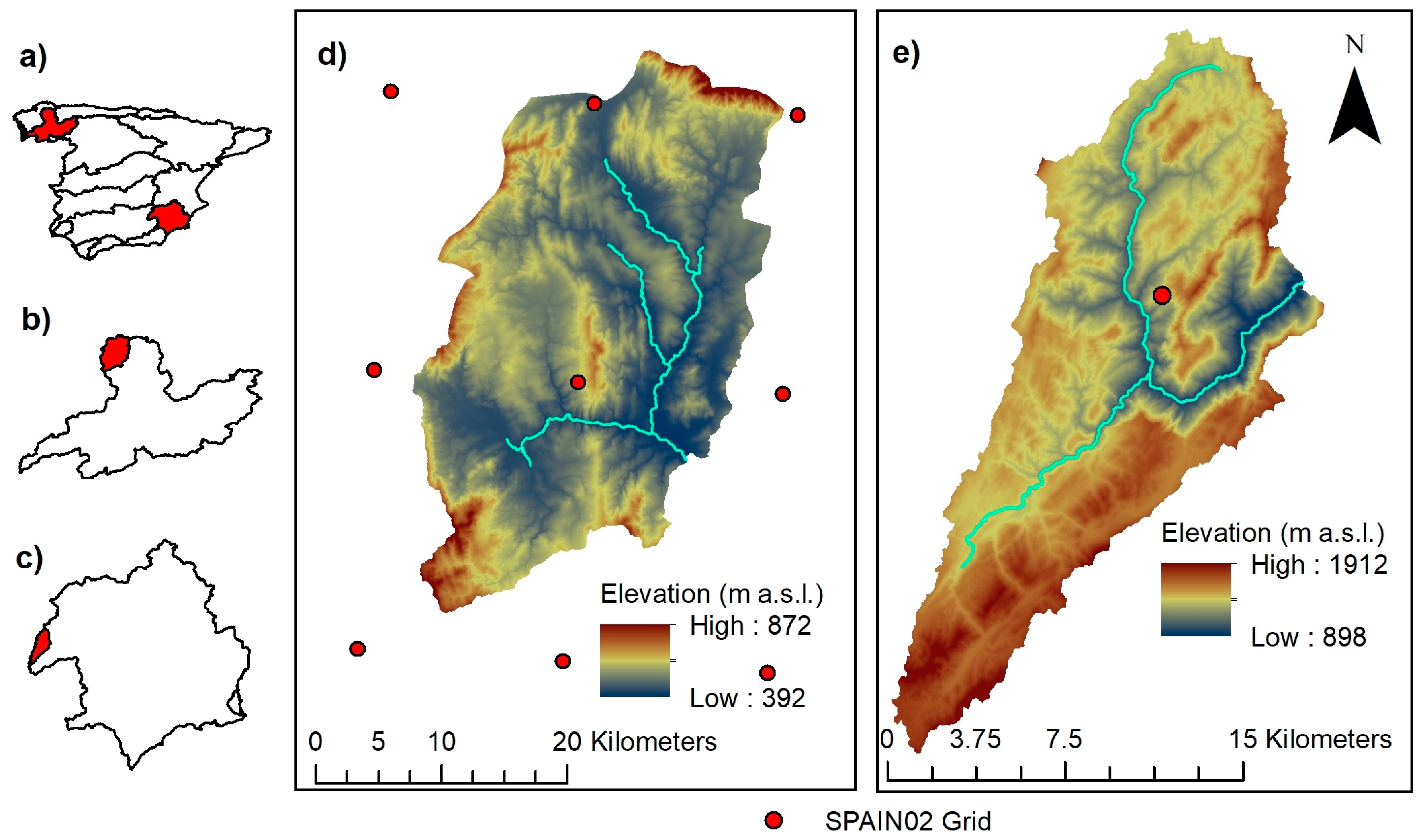
Determining the input variables has a significant influence on the simulated flow. The basin rainfall and temperature data used by the ANNs were calculated using the Thiessen method, in which the climate values were based on a weighted average of the contribution of the cell in the area. After reviewing other research [
22,
23,
48], we have selected the following variables as inputs to the ANN models to estimate daily streamflow: daily precipitation (P
t), daily temperature (T
t), precipitation of the previous
n days (P
t−n), total rainfall of the preceding
n days (R
n) and mean temperature over the previous
n days (Tm
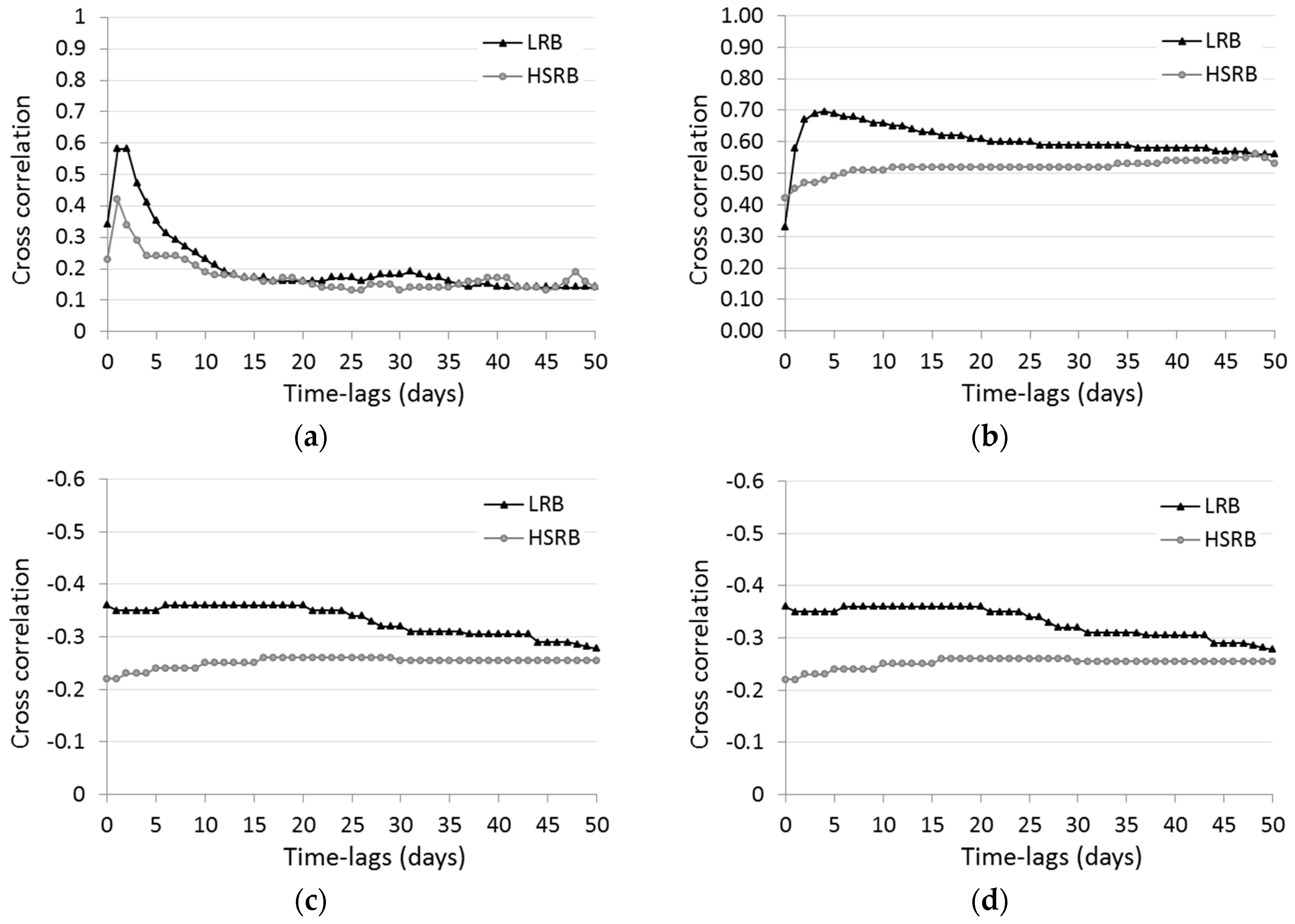
n). In this study, the most suitable delays of climate variables were determined using cross-correlation analyses, so we determined the temporal relationships between these input variables and streamflow. As shown in
Figure 2a, the streamflow is highly positively correlated with daily precipitation of the current day
t (P
t) and with daily precipitation of the previous days, until
t-4 for LRB and until
t-2 in HSRB.
Streamflow is strongly correlated with accumulated daily rainfall; there is a greater correlation for 4 days in LRB and for 48 days in HSRB, reflecting the little and the great importance of groundwater, respectively, in these basins. With respect to the daily temperature, there are moderate negative correlations with the daily streamflow in both basins. Finally, a total of four input combinations have been proposed for each basin in this study (
Table 7).
For the network structure identification, we implemented and built the ANNs using MATLAB
® software (version 8.2.0.701 (R2013b), The Mathworks, Natick, MA, USA). A multilayer feed-forward network was used. The number of hidden layers and hidden neurons was established by trial-and-error procedure; one or two hidden layers with a number of neurons between two and ten are considered. The number of neurons in the input layer depends on the number of input variables in each scenario, which varies from 3 to 7.
Figure 3 shows the ANN structure used in this work.
The different scenarios defined in
Table 7 were tested for determining the type and number of inputs to ANN models.
Table 8 shows the best architecture of ANN and their performances for each scenario trained and validated for the studied basins. These performance measures values are averages obtained over the five rounds of cross-validation.
The results shown in
Table 8 indicate four effective ANN structures with good performances for LRB. Scenario 1 for LRB with a combination of six cells in the input layer (the precipitation of days
t,
t-1,
t-2,
t-3 and
t-4, and the temperature of day
t), one hidden layer with two neurons and one neuron in the output layer (the streamflow of day
t) had the highest NSE and the lowest RMSE in the training and validation phase. Based on the criteria of
Table 3, NSE and PBIAS of scenario 1 were good and very good, respectively. Therefore, scenario 1 was the selected architecture for LRB. However, the performance levels of ANN models for HSRB were lower in general because modelling the hydrological response of arid and semi-arid regions, where evapotranspiration rates are high and precipitation is irregular and/or limited, is especially complex [
61]. The selected model for HSRB was scenario 3 where NSE and RMSE were better than those obtained in other proposed scenarios. In this scenario, NSE was classified as satisfactory and PBIAS as very good. The rest of the scenarios were classified as unsatisfactory based on NSE. Therefore, the ANN configuration selected for HSRB was three cells in the input layer (the precipitation of days
t and
t-1, and total rainfall of the preceding 48 days), one hidden layer with four neurons and one neuron in the output layer (the streamflow of day
t). In conclusion, the structure selected for both basins was formed by three layers, similar to other studies (e.g., [
1,
23]).
3.3. Comparison of Model Performance
Calibration of SWAT models and training of the selected ANNs (scenario 1 for LRB and scenario 3 for HSRB) were done using the training data sets (1971–1989 for LRB and 1987–1997 for HSRB). Then, we tested the models with the validation sets (1990–2007 for LRB and 1998–2007 for HSRB). A comparison of flow estimation performance of the SWAT and ANN for LRB and HSRB is provided in
Table 9, which shows separately the performances for the calibration/training and validation periods.
The values of NSE for both models were classified as good according to the criteria listed in
Table 3 for the calibration/training phase in LRB and HSRB. For the validation phase, the NSE values ranged between 0.5 and 0.7, and therefore, they were classified as good for both models of the LRB. The NSE values were classified as satisfactory for both models of the HSRB. The PBIAS values were less than 25%, so they were classified as very good in all cases. The values of RMSE for both models were similar. The NSE and R
2 values obtained by the ANN model were higher than those obtained in SWAT in both basins, and those during training were higher than those during validation phases. After analysing these results, it was concluded that both SWAT and ANN were suitable. The more arid the catchment, the lower the performances obtained in the hydrological models, which is similar to the experience reported by Pérez-Sánchez et al., (2017) [
61].
For a better understanding of the difference between the models,
Figure 4 shows the results of SWAT and ANN models plotted against the observed values of streamflow for the calibration/training and validation periods with their correlation coefficients.
SWAT models had a poor performance in estimating the large values of streamflow, whereas ANN models were worse in estimating the small values. In every figure of
Figure 4, the points which are related to streamflow with large values are positioned at a greater distance to the 1:1 line when the values have been estimated by SWAT. In contrast, the points related to the estimated streamflow by ANN models are farther from the 1:1 line when it comes to the estimation of small values.
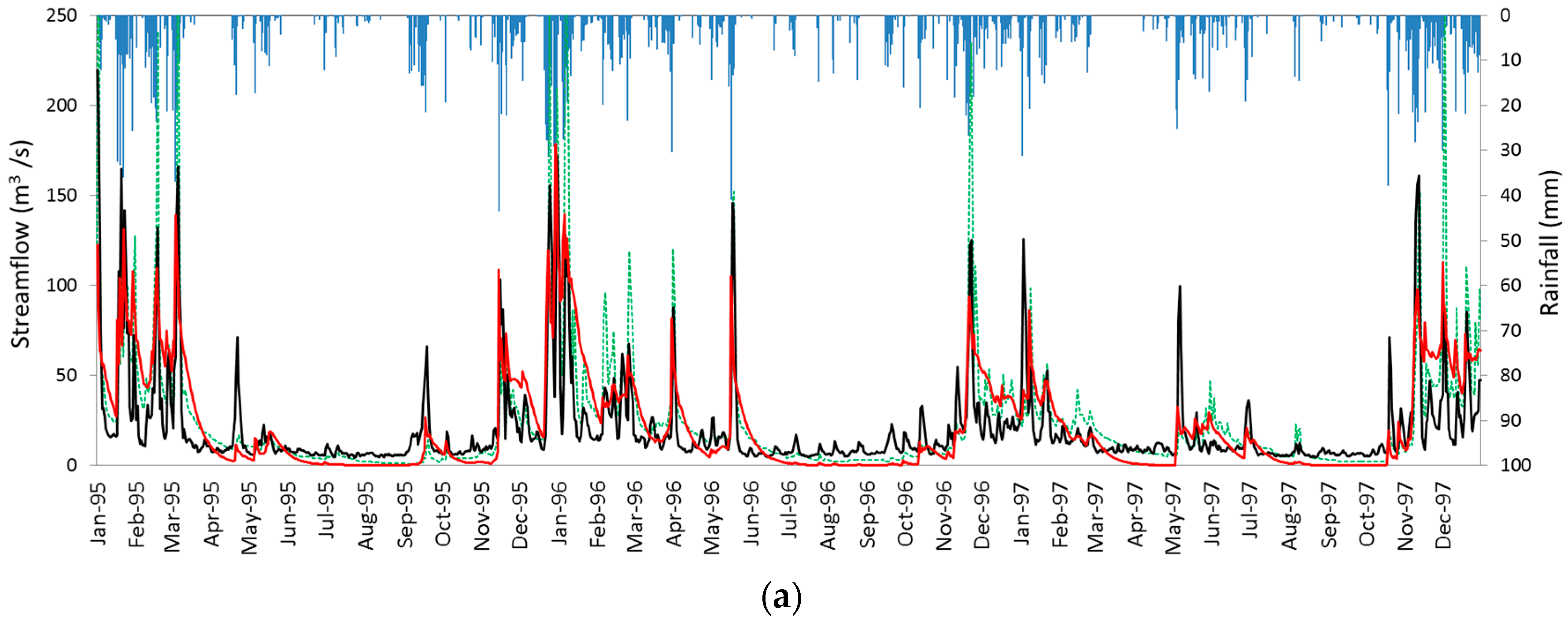
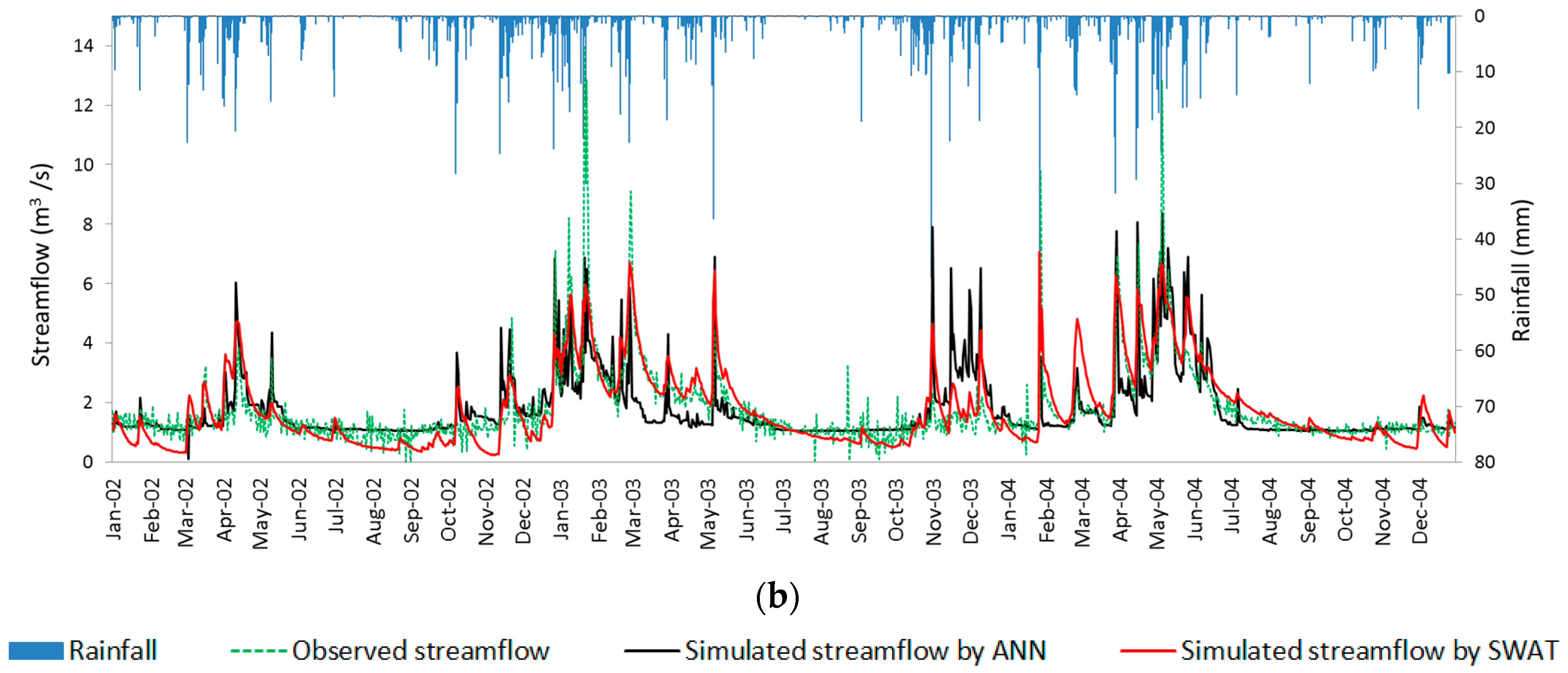
The hydrographs (
Figure 5) show the fit obtained for simulated versus measured streamflow in the studied basins during the validation period (from 1995 to 1997 for the LRB and from 2002 to 2004 for the HSRB). The models generally reproduce the streamflow fairly well. Although both models tended to underestimate the peak-flow events during the validation phase, ANN models were more sensitive to precipitation events than SWAT models, and their estimations always remain above those obtained by SWAT.
According to Chen and Chau (2016) [
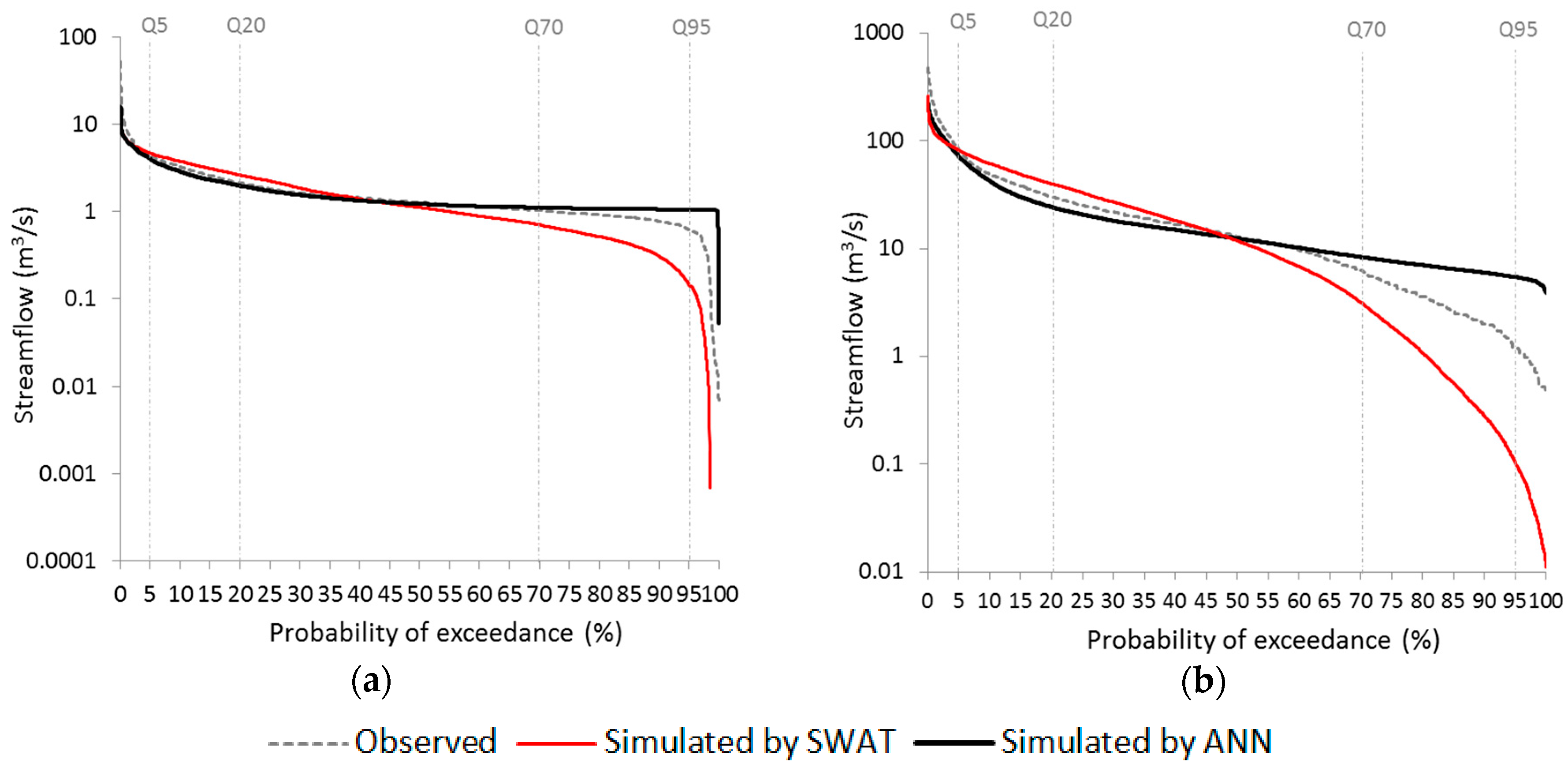
11], NSE and RMSE scale the mean squared error of estimation models, therefore they particularly reflect the performance on high values. Thus, the above discussions on evaluation criteria and plots of estimated data could not provide explicit performances on different intervals of values. To address this problem, different ranges of flow (from very high to very low flow) were determined. The reproduction of the streamflow was analysed by the FDC of LRB and HSRB for the validation periods (
Figure 6). The FDC for LRB shows that the ANN performed generally better in the very high flow segment and SWAT was better in the very low flow segment. The values obtained by SWAT and by ANN were graphically similar for the rest of the flow segments in LRB. For HSRB, SWAT was better only in the very low flows.
An analysis of performance based on RMSE in each hydrograph phase was also done, as reflected in
Table 10. The best results for each basin are highlighted in bold. As it was expected, high peaks are better simulated at the expense of low flows due to the fact that RMSE is biased towards high values. The RMSE values suggest that the SWAT model was better in the estimation of very low flows and ANN in the estimation of very high flows in all cases.
Similar results regarding peak-flow inefficiency of SWAT have been obtained in other studies (e.g., [
5,
22,
23]), which suggested that peak-flow inefficiency could be caused by the formulation. The results obtained show that use of ANN models can help reduce the error in the estimation of high streamflow values, although these were also underestimated. One of the reasons is that the data of high values are scarce in the training data sets, the medium and low values being more numerous as illustrated in the cloud of points in the scatterplots in
Figure 4. This problem in the application of neural network has also been reported in the works of Minns and Hall (1996) [
15] and Talebizadeh et al., (2010) [
62]. On the other hand, SWAT models simulated the estimation of the low flow values better than ANNs. In general, ANN models tended to overestimate the low values of streamflow. This inability can be attributed to complex non-linear relationships governing the process of low flow, often related to the base flow from groundwater. The performance of the ANN could be deteriorated with the increase in non-linearity [
15]. It is generally accepted that the processes of streamflow generation are likely to be quite different during low, medium, and high flow periods. The base flow mainly contributes to low flow events whereas intense storm rainfall gives rise to high flow events [
63]. Therefore, a single global ANN model could not predict the high and low runoff events satisfactorily [
15]. SWAT models may obtain satisfactory results for the estimation of low flows but could not simulate very high streamflow with the same accuracy. In contrast to SWAT, a single ANN can obtain better results for very high values but not for the lowest values; these results are similar to those obtained by Kim et al., (2015) [
23]. Therefore, the use of these models is suitable for simulating the streamflow in a basin. In the case of studies of extreme hydrologic events (e.g., floods), it is recommended to use an ANN model to simulate high-flow events. Otherwise, in studies of hydrological management in which low-flow events are more interesting, applying the SWAT model would be more desirable. In addition, it is important to take into account the disadvantages of each model. In Spain, it is relatively easier to obtain the input data, such as the streamflow and precipitation data, for the ANN model through the governmental online resources compared to data regarding the physical characteristics of river basins, such as soil moisture, infiltration, soil classes, groundwater level and evaporation, for the SWAT model. In addition, the time consumed in the setup and calibration of SWAT is higher than that consumed in the implementation of an ANN model. However, an ANN is a black box, and the water balance and its components are not obtained. The use of precipitation and temperature as the only inputs of the models is, on the other hand, a limitation of the ANN models used because the rainfall-runoff relation is impacted by different physical parameters too. The non-consideration of land use or land management in the ANN model makes the SWAT model more advantageous if a number of scenarios are to be made to investigate the response of the basin [
1].
The results of this study suggest, however, that the ANN approach is very efficient to simulate a hydrological process because it requires very few input variables and minimal resources to implement and therefore, it is sufficiently promising to the development of other approaches such as the simulation of water quality process, as it is reflected in some studies (e.g., [
64,
65,
66]).


 ,
, 


