1. Introduction
As generally acknowledged, infrastructure is becoming more and more important to keep cities functioning. In order to maintain the desired level of serviceability the infrastructure has to be properly maintained and rehabilitated [
1,
2]. Two important parts of the infrastructure for human wellbeing are water supply networks and sewer systems. These systems are essential for public health and preventing epidemics. As the infrastructure is ageing there is wide felt need for strategy development for maintenance and rehabilitation.
Sewer systems and water supply networks are underground infrastructure; therefore it is not straightforward to determine the actual condition of the assets. The maintenance and rehabilitation of sewer systems is often solely based on the results of visual inspections (see [
3]). Studies have been carried out to develop methods for optimizing the locations and frequencies of visual inspections. A generally used optimization concept is the combination of the likelihood of failure (LoF) with the consequence of failure (CoF) (see e.g., [
4,
5,
6,
7,
8,
9,
10,
11]). The likelihood of failure is often related to the soil type, the load on the system and the material type where the consequence of failure is often related to the conduit characteristics (e.g., conduit size, conduit depth) and the location of the conduit in the urban area. The criteria and weights of the criteria used in decision support methods for the prioritization of rehabilitation project influences the outcomes of the decisions [
12].
Sewer systems and water supply systems are networks consisting of many elements. The performance of the network depends on the functioning of the individual elements. The importance of an element for the network depends on the characteristics of the element and its position in the network.
If the degree of criticality of the elements in a network is known, the maintenance and rehabilitation can be adjusted accordingly to the degree of criticality instead on maintaining all elements to the same quality level. The criticality can also be combined with the consequences of failure. Failure of (sewer) systems has impact on the service level (drainage of water) and on the surrounding (health risks, floods, blocked roads, damage to other infrastructure). The degree of criticality can therefore be used as a basis for risk-based asset management. It can be used to analyse the robustness of a network and to evaluate measures to increase the robustness as well.
Only a limited number of methodologies on how to determine the importance of the individual elements in relation to the complete network is described in literature. Arthur and Crow [
4,
9] describe a methodology to identify critical assets. This methodology is based on surcharged capacity, combined with surcharging water level, and is applicable to gravity systems. A second method, called the Achilles approach, is used in the planning tool for the identification of weak points during operation and emergency for the urban water infrastructure [
13,
14,
15,
16]. In this approach, the capacity of each conduit in a hydrodynamic model is reduced to (almost) zero and the hydraulic consequences are determined. For large (> 5000 conduits) (looped) systems both methods require a large calculation effort.
This paper proposes a new approach towards identifying the criticality of individual components in water related networks such as sewer systems. The proposed graph theory method is independent of the load on the system and requires limit calculations effort. This article focuses on sewer networks but the described approach has a wider applicability (e.g., drinking water networks). First, the theory of the method and an existing method to compare with is presented; secondly, the existing method is tested for various storm events; thirdly, some examples of both methods are presented based on urban drainage networks and the results and performance are compared with the traditional method; and finally, the results are discussed and conclusions and recommendations are formulated.
2. Materials and Methods
2.1. Studied Sewer Systems
Sewer systems are gravity-driven systems. During dry weather conditions, all the water is drained to pumping stations that transport the water to waste water treatment plants. During storm events, water is partly drained to the pumping station and partly to surface water via combined sewer overflow structures (CSO). In general, the pump capacity is limited (in the Netherlands, the capacity is circa 0.7 mm/h), meaning that during (extreme) storm events most of the water is drained via CSOs. Because water can flow both to pumping stations as well as to CSO, the flow direction can revolve.
For the sewer systems Loenen (the Netherlands) and Tuindorp in Utrecht (the Netherlands), the degree of criticality of the conduits are determined. Both systems have been used several times in other studies and are also extensively calibrated [
17,
18,
19,
20].
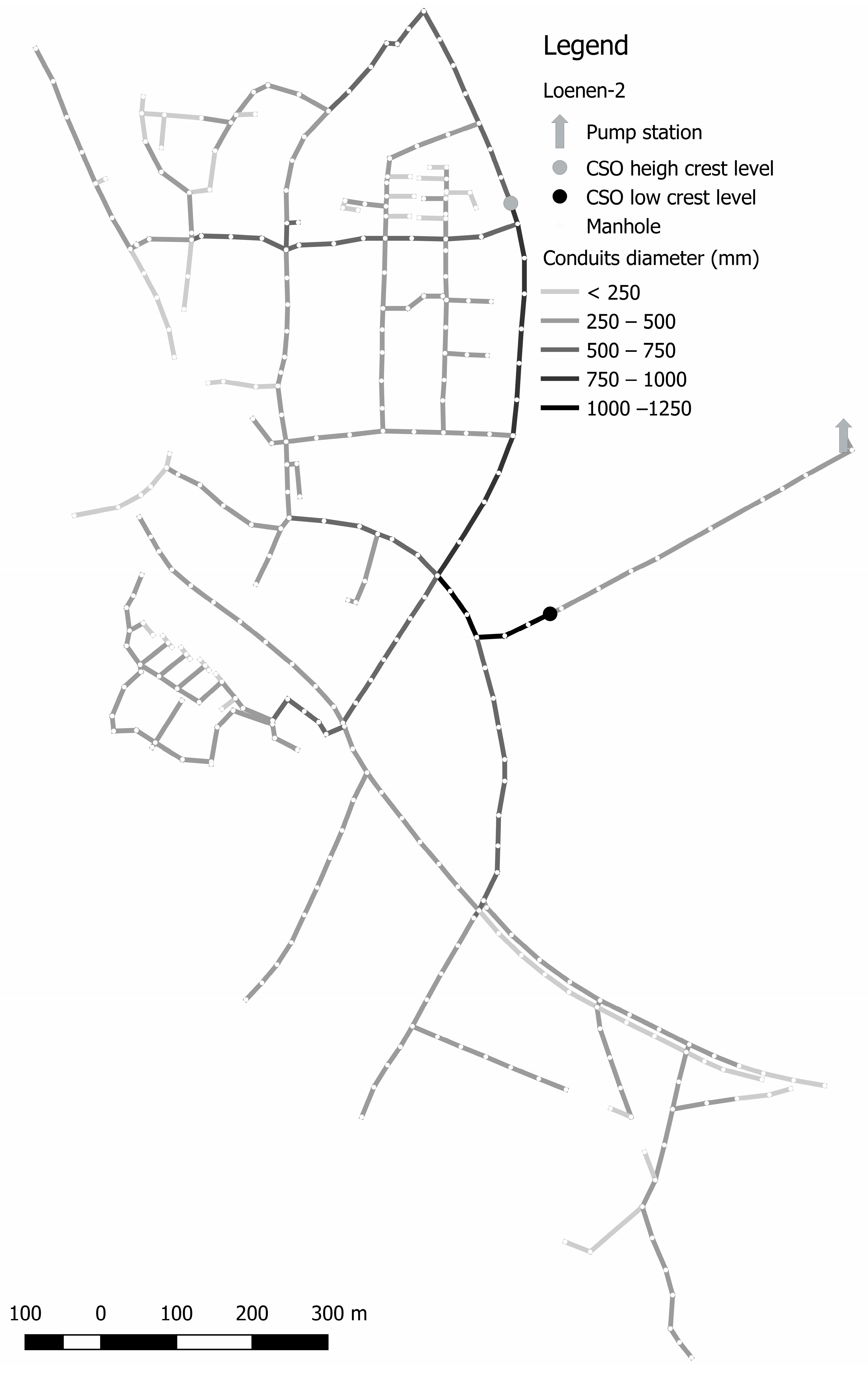
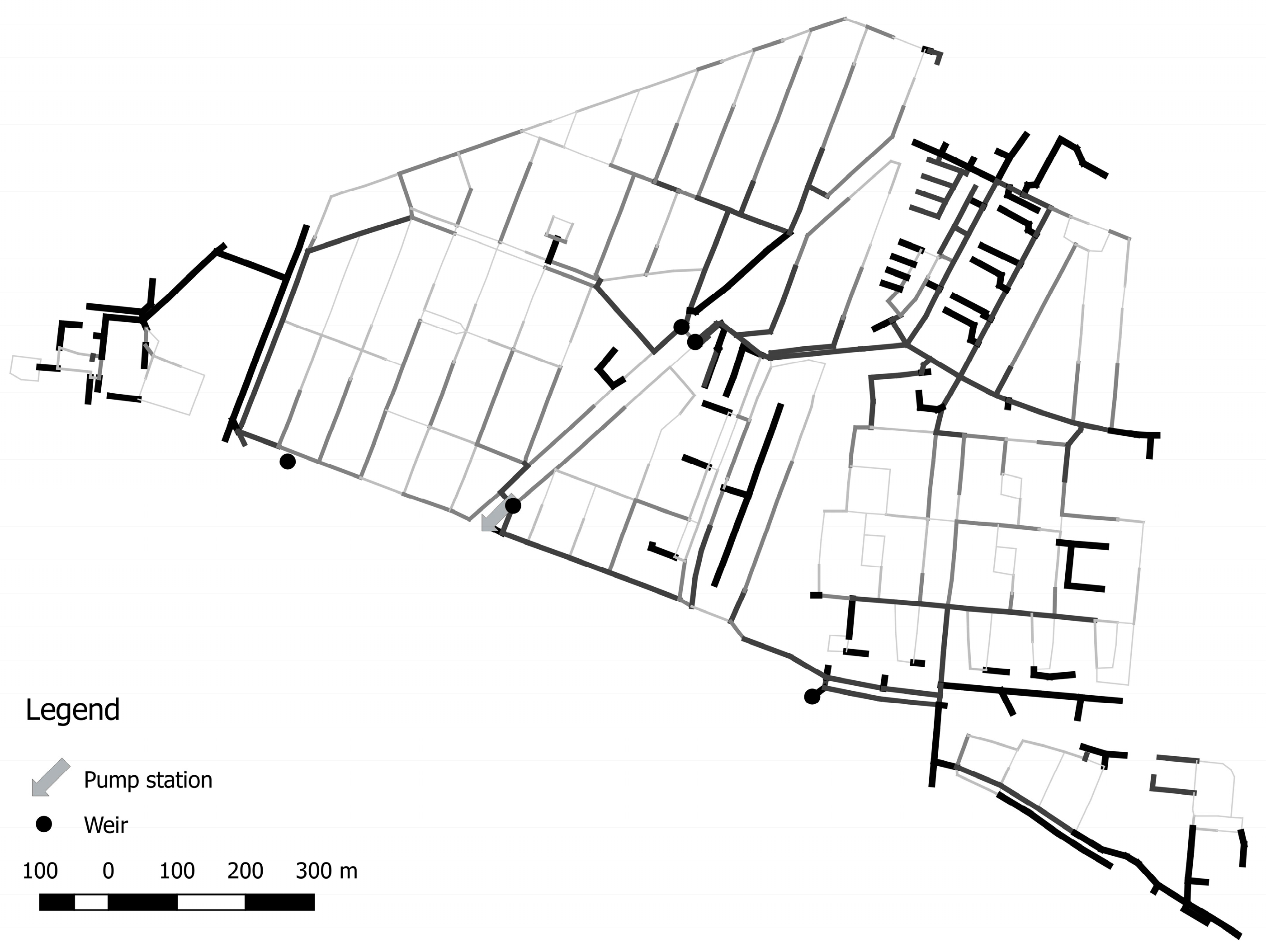
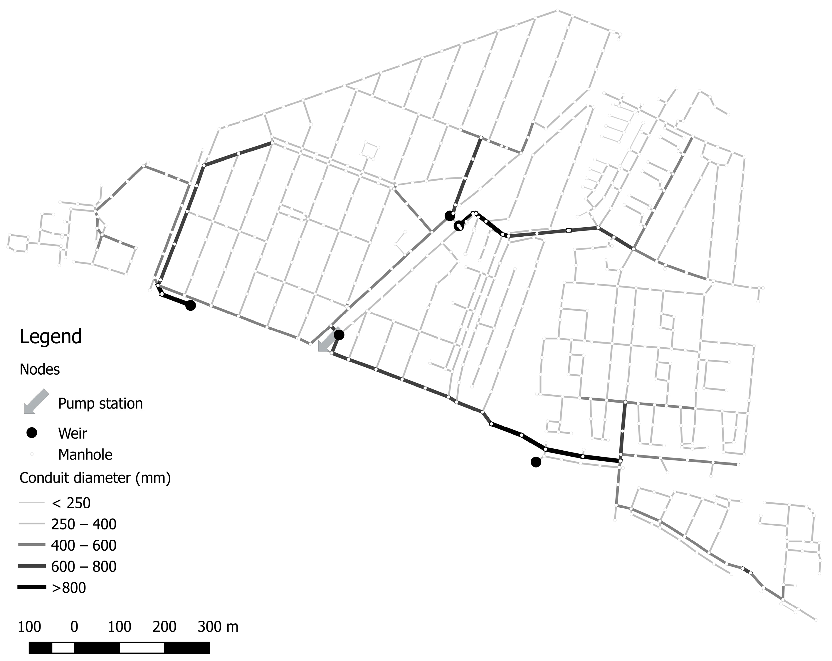
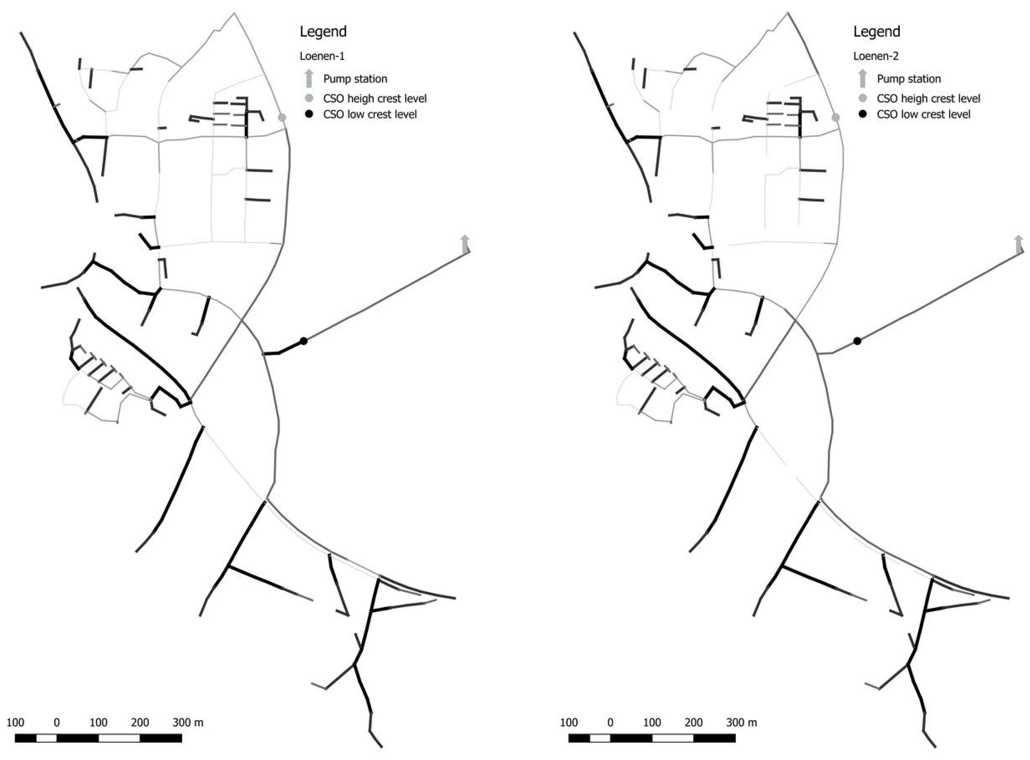
Table 1 shows the characteristics and
Figure 1 and
Figure 2 show the layout of the systems. For the Loenen catchment, two situations are studied: Loenen-2 including both CSO’s structures, and Loenen-1, where a weir that only becomes active during storm events with high rainfall intensities is closed.
2.2. Used Storm Events in the Simulations
Simulations with the models have been made with different types of storm events. The 10 design events from the Dutch national guidelines for hydrodynamic modelling of urban drainage systems [
21] are used. The events vary between 10.5 mm in 75 min (maximum intensity 40 L/s.ha. (14 mm/h) to 35.7 mm in 45 min (maximum intensity 210 L/s.ha (75.6 mm/h)). The most commonly used stationary design storm events in the Netherlands 40, 60 and 90 L/
s.ha (14, 21.6 and 32.4 mm/h) are used for Loenen-1 and Tuindorp. For Loenen-2, 10 storm events are used with a stationary rainfall intensity varying from 10–100 L/s.ha (3.6–36 mm/h) during 24 h. For Tuindorp, 13 storm events are also used of the rainfall series observed by the Royal Dutch Meteorological Institute in De Bilt over the period 1955–1964.
In earlier research, Monte Carlo simulations were applied to systematically study the impact of in-sewer defects on hydraulic performance of the Tuindorp catchment. Because it is not possible to predict which storm event results in flooding in the model simulations due to the changes in the characteristics of the network during each run in the Monte Carlo procedure, long-term rainfall series were used instead of predefined storm events. Using a filtering approach, 41 independent storm event were selected (see [
17]).
In addition, a selection of conduits has been applied to determine the impacts on hydraulic performance. The conduit locations have been chosen based on the system layout and expert judgement. This resulted in a total number of 198 conduits. In the hydraulic simulations regarding pluvial flooding, the diameter of the selected conduits has been reduced one by one to 10% of the original conduit diameter.
The total calculation time for the Tuindorp system based on the filtered storm events and conduit selection was 273 h. It is obvious that this is a time consuming method for this looped system. Therefore, only 13 storm events that caused flooding are used in this research.
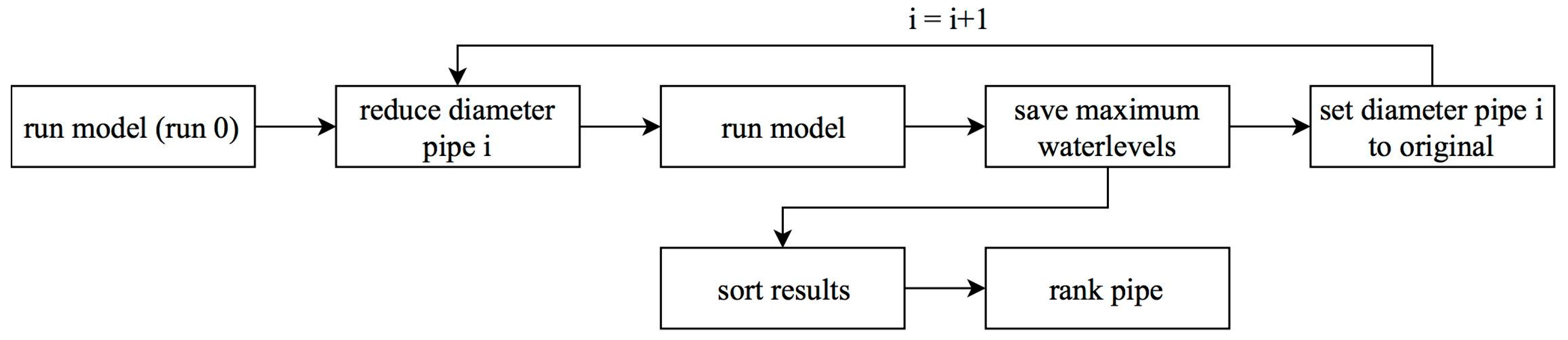
2.3. The Achilles Approach
A general, applicable method to determine the criticality of an element in a sewer system is shown in
Figure 3. This method is part of the Achilles approach [
13,
14]. The Achilles approach can be used to determine vulnerable sites of water infrastructure. For the identification of vulnerabilities the outcomes of a hydrodynamic model are used (hydrodynamic model method, HMM). First, a simulation is done with the original model in which all conduits function well. After this, the diameters of the conduits are one by one reduced to zero to simulate a blockage. For every blocked conduit, a simulation is carried out so the number of simulations is equal to the number of conduits plus one. The results are compared based on the increase of the calculated ponded volumes. The reduced conduit diameter that causes the largest increase in ponded volume is the most critical pipe.
In literature about the Achilles approach, two methods to sort the results are used. The first method is a performance indicator based on the maximum ponded volume and the total rainfall runoff (Formula (1) (an explanation of the symbols used can be found in the list of symbols)) [
14]. The main assumption of Möderl [
14] is that the performance indicators are independent of the rainfall events. Formula (2) (Method 2) shows a performance indicator that indicates the probability of damage caused by flooding [
13].
In which
| c = Catchment | (-) |
| F = Probability of damage cause by flooding | (-) |
| #J = Nr of Junctions | (-) |
| N = Node | (-) |
| PI = Performance indicator | (-) |
| VP = Ponded Volume of each node | (m3) |
| VR = Total rainfall runoff volume | (m3) |
| x = Flooding volume | (m3) |
The hydrodynamic model method (HMM) will be used as benchmark for the outcomes of the method based on the graph theory. The method described by Arthur and Crow [
4] is not applicable for fully surcharged systems and this is often the case in flat areas like the Netherlands and therefore not used.
Application of the Hydrodynamic Modelling Method as Reference Method
The outcomes of the traditional hydrodynamic model method (HMM) (see
Figure 3) are used as reference for the degree of criticality based on the graph theory method (GTM). In the GTM, it is possible that a node no longer is connected to a part of the network with a sewer overflow after a conduit is deleted (see
Section 2.4 and
Section 2.5). This can cause problems in the simulations of the HMM, and therefore the conduits are not deleted but the diameter is reduced to 10 mm (the minimum allowed diameter in the software package).
When a part of the network is not connected to a CSO because of a blocked pipe, floods will occur at every storm event. The severity of the blockage depends on the area that is disconnected from the CSO. The blocked conduits that lead to “unconnected nodes” are ranked based on the runoff surface connected to these nodes. After that the other conduits are ranked based on the results of the HMM.
In each run of the HMM, the diameter of one conduit is reduced to 10 mm. When the increase in water levels is divided into categories to rank the links the outcome of the ranking depends on the used categories. Therefore, the links are ranked based on the increase in flood volume and the increase of water level in the sewer system. After each run, the increase in flood volume and the increase of water level, relative to the original model, are determined for each manhole. The results of all manholes are summed and the links are sorted: first based on the total increase in ponded volume and then on the total increase of water level. The conduit with the largest total increase in the flood volume is ranked as most critical after the conduits that cause “unconnected nodes”. If the increase in flood volume is the same for two conduits, the conduits are sorted based on the increase in water level.
There are two differences between the HMM as described in the Achilles approach and used in this research. The first difference is the use of a minimum diameter of 10 mm instead of a fully closed pipe. The effect of this adjustment is described in the section of the results. The second is the method to rank the conduits. Instead of ranking the conduits between 0–1 based on the ponded volume and the rainfall runoff (see Formula (1)), the conduits are ranked based on the surface that is disconnected, the increase in ponded volume and the increase in water level. For the blocked conduits that cause flooding, this adjustment will not influence the ranking and this adjustment makes it possible to rank all conduits including the blocked conduits that do not cause flooding.
To validate the assumption of the Achilles approach that the performance indicators are independent of the rainfall events [
14] the HMM is used to determine the degree of criticality for various storm events (see
Section 3.2).
2.4. Introduction to Graph Theory
The graph theory is a mathematical theory and is widely used in, for example, route problems and optimization of flow problems. A graph consists of nodes and links. Graphs are used to represent relations in for example physical, information and social systems. Leonhard Euler laid the foundation of the graph theory in 1736 with the Königsberg bridge problem [
22].
A graph can be used to simplify a network and its connectivity in nodes and links [
23]. Networks such as water supply networks, sewer systems, electricity networks are typical examples of graphs consisting of links (conduits, cables) and nodes (connections or manholes). In hydrological models graphs are used to represent the structure of the network. There is little literature known about the use of the graph theory to analyse criticality of conduits in sewer networks (e.g., Laakso [
24] used the cut-edge analysis to reveal sewers that serve a high number of connections).
A graph G = (V, E) is a set V of nodes and a set E of links formed by pairs of nodes [
25]. A path in a graph between a source node and a target node is a route between the source node and the target node without a node occurring more than once. Each link can have a weight, costs or penalty. The term most often used is costs and is adopted here as well.
The costs in, for example, a road network can be defined as the distance between two places, the speed limit, the toll, fuel consumption or the risk of getting stuck in a traffic jam. The costs are a metric for determining shortest or cheapest paths. For piped water systems the necessary amount of energy to transport the water (head loss) is utilized as costs. This is explained in more detail in the paragraph Costs of links sewer system (
Section 2.5.1). For the graph in
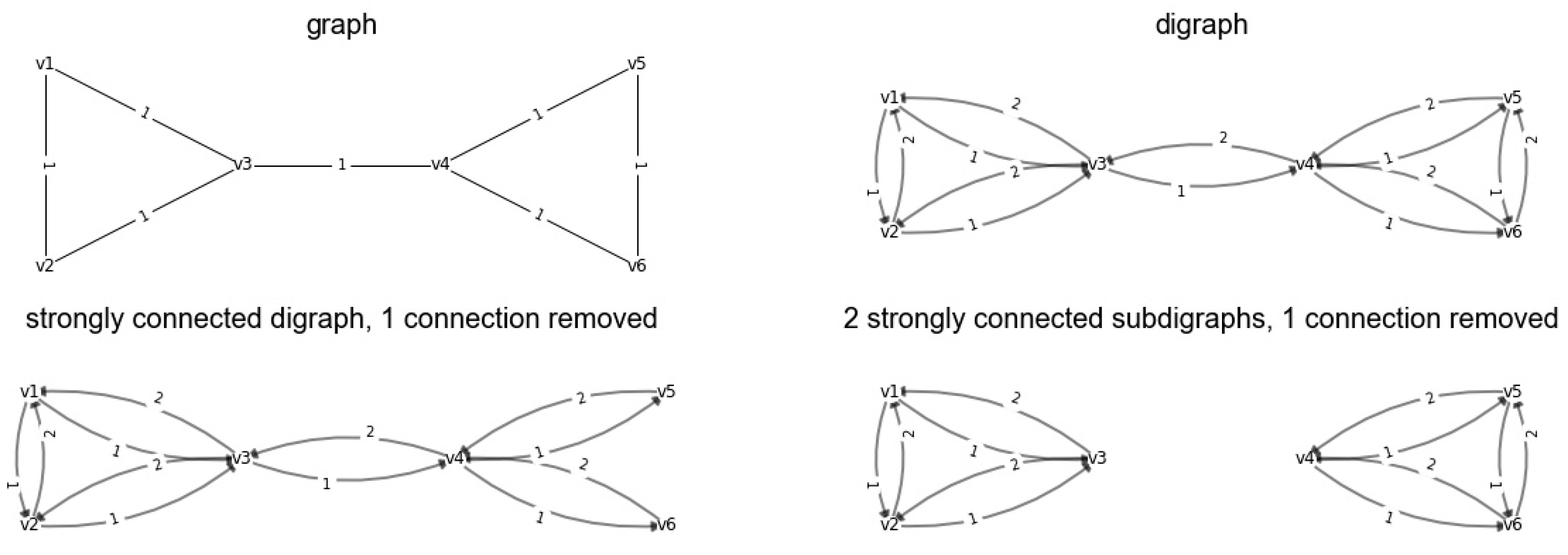
Figure 4 a path v1–v6 is v1, v2, v3, v4, v5, v6 (costs = 5) and the shortest path v1–v6 is v1, v3, v4, v6 (costs = 3).There are different kinds of graphs. The upper left graph in
Figure 4 is a graph in which v1, v2 = v2, v1. This graph can be used when the costs of opposite flow directions in a conduit are the same, in this example the costs are 1.
A directed graph or digraph is formed by nodes connected by directed links. In a digraph the link v1, v2 ≠ v2, v1 while in a graph v1, v2 = v2, v1 (see
Figure 4, digraph). A digraph can be used when the costs of opposite flows are different. In this example the costs of the edges in positive direction are 1 and in the negative direction are 2. When all nodes in a directed graph are connected in two directions, it is called a strongly connected graph. The removal of a conduit can result in one or more strongly connected digraph(s). The lower left graph in
Figure 4 shows the situation in which the connection v5, v6 and v6, v5 is removed and the result is a strongly connected digraph. The lower right graph in
Figure 4 shows the situation in which the connection v3, v4 and v4, v3 is removed and the result is two strongly connected sub-digraphs.
2.5. The Graph Theory Applied on Sewer Systems
The graph theory is applied as a concept to determine the degree of criticality of a conduit during storm conditions. The sewer system is represented as a digraph. Each manhole is represented as a node and each conduit as a link. Between each pair of nodes two links are used, each with its own costs. This allows making a distinction between a positive and negative flow direction (
Figure 4, digraph). This is necessary because a blockage of a link can result in a reversed flow.
During storm events most of the water flows out of the sewer systems via a combined sewer overflow (CSO). For each node (source), a path is determined to one of the overflows (targets) in the sewer system. Each path has its own length or “costs” (see
Section 2.5.1. Costs of links sewer system). For each node, the cheapest path to the combined overflow structure is determined based on the Dijkstra algorithm [
26].
The Dijkstra algorithm is a widely used algorithm. The general principle is to assign to every node a tentative distance value (source = 0, target = ). The source node is marked as active and the other nodes as unvisited. The tentative distances are calculated to all neighbors’ nodes of the source node. The smallest of the newly calculated tentative distance and the currently assigned tentative distances are assigned to the node. When all the distances between the source node and the neighbor nodes are calculated the source node is marked as visited. The unvisited node with the smallest distances becomes the new active node. The process continues till all unvisited nodes are visited or the target node is reached.
For each node the costs of the shortest path to the combined overflow structure is multiplied with the runoff area connected to the source node. The total costs of a graph are determined for the complete graph by summing the costs of all nodes to a combined overflow structure (Formula (3)). To determine the criticality during dry weather conditions the target is a pumping station instead of a combined overflow structure.
In which:
| Ai = the surface connected to the source node | (ha) |
| Cgraph = costs of the graph | (-) |
| Cvi−vn = the costs of the shortest path from vi to target vn | (-) |
In case of more than one overflow structure in a sewer network, each node has multiple targets. In such a case, the costs of all nodes to all targets are calculated. For every node the lowest cost of the path from the node to an overflow is used to determine the total costs of the graph.
To reduce the calculation time the calculations are not carried out from the source to the target node but from the target(s) to all nodes. Therefore, the positive and negative conduit costs are turned around to obtain the right total costs.
After calculating the total costs of the complete graph, a connection between a pair of nodes is deleted to simulate a conduit blockage (see lower images in
Figure 4). This implies that the edges v
x,v
y and v
y,v
x are deleted. When all nodes are connected the new graph remains a strongly connected digraph (
Figure 4 lower left). Otherwise the result is two strongly connected sub-digraphs (
Figure 4, lower right). Two situations are possible. First, all (sub-) digraph(s) contain at least one target node. Second, only one of the sub-digraphs contains at least one target node. If the first situation, the total costs of the (sub)digraph(s) are determined. If the second situation, the runoff surface is summed of the nodes that are not connected to a target (see
Section 2.4).
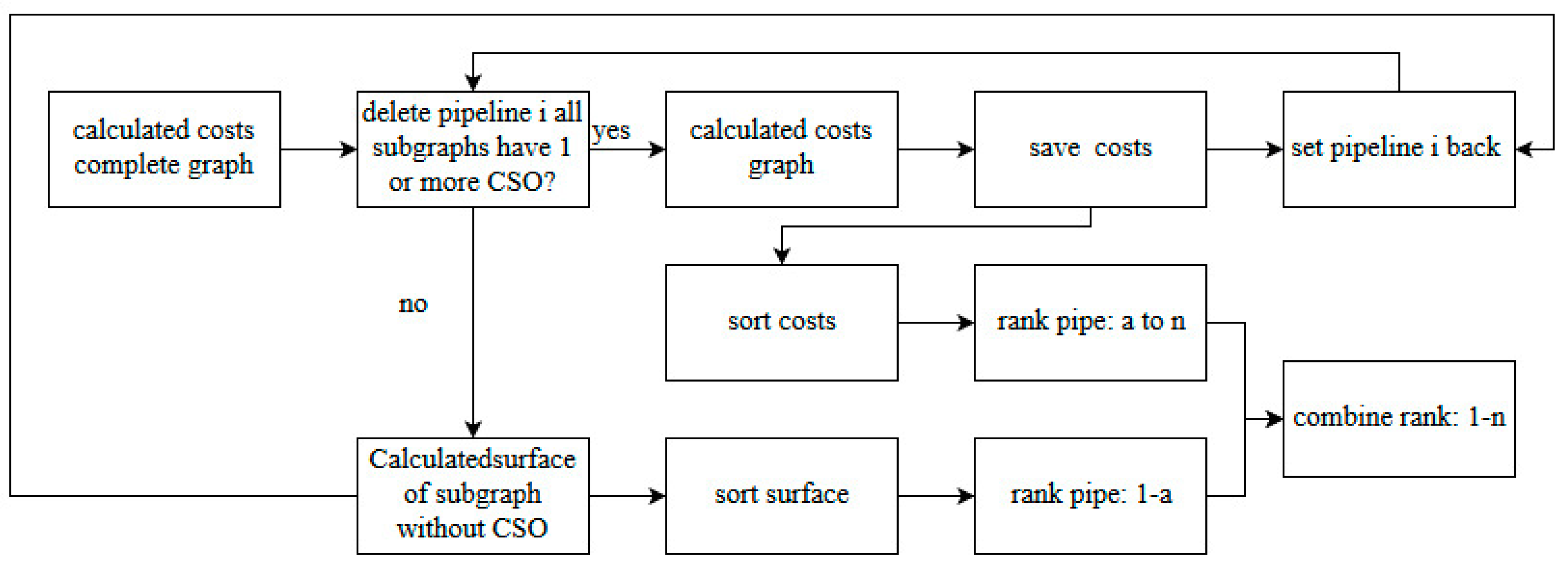
The process as shown in
Figure 5 is applied. The result is a list of deleted connections with the total costs of each digraph or the runoff surface that is not connected anymore to a target. The deleted connections are sorted, firstly by the amount of runoff surface that is not connected to a target, secondly by the total costs of the digraph from large to small amount of runoff surface and from high to low costs. The deleted connections are ranked from 1 (most critical connection) to the total number of edges (less critical).
2.5.1. Costs of Links Sewer System
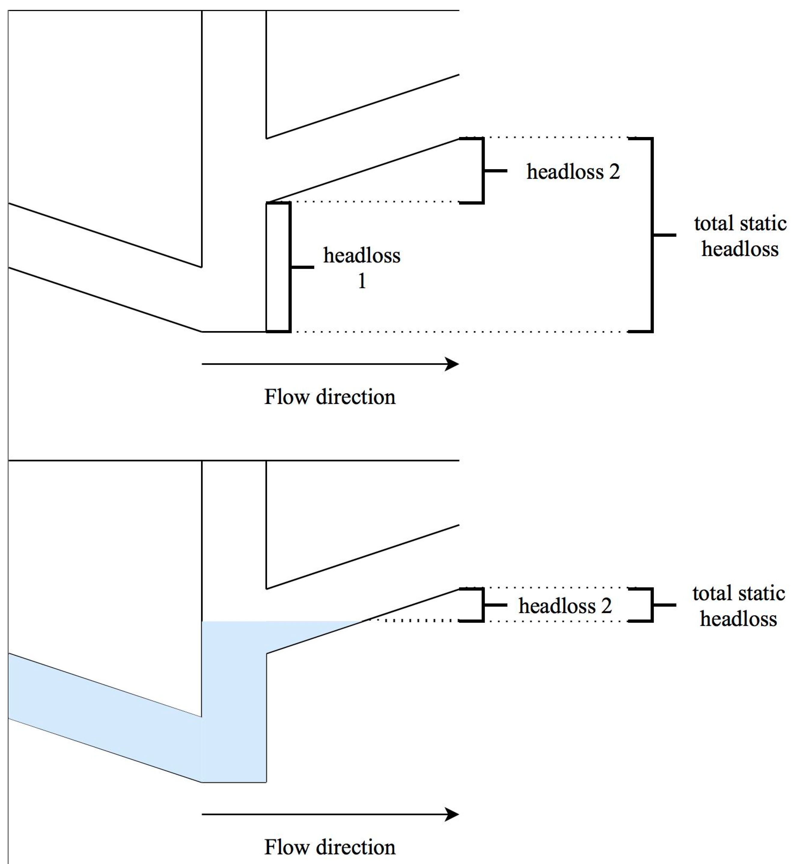
The links’ costs are derived from the head loss in a link. The head loss is the amount of energy needed to transport water from point A to point B. The head loss comprises two parts. The first part is the static head and is the amount of energy needed to lift water. The amount of energy is equal to height differences between A and B. The second part is the dynamic head. Energy is needed to let water flow from A to B. The amount of energy that is lost due to the resistance of water to flow between A and B is expressed as the dynamic head loss. The dynamic head loss depends on the characteristics of the liquid and the conduit dimension and hydraulic characteristics.
In a gravity sewer system, the head loss comprises a dynamic part and two static parts (see
Figure 6). The first static component is the height difference between the water level in the manhole upstream of the conduit and the upstream invert level of a conduit. If the water level in the manhole upstream of the conduit is higher than the upstream invert conduit level this value is zero. For the water level in a sewer system the crest level of the CSO with the lowest crest level of the system can be used. The second static component is the height difference between the upstream and downstream invert level of the pipe. If the water level is higher than the invert level this value is zero. If the downstream invert level is lower than the upstream invert level the value is also zero.
The dynamic head loss in a conduit is described with the following formulas:
In which
| A = area of pipe | (m2) |
| C = Chézy coefficient | (m1/2/s) |
| ΔH = head loss | (m) |
| k = wall roughness | (m) |
| L = length | (m) |
| q = discharge | (m3/s) |
| R = hydraulic radius | (m) |
2.6. Comparison of Criticality between Hydrodynamic Model Method (HMM) and Graph Theory Method (GTM)
The Kendall rank correlation coefficient [
27], commonly referred to as Kendall’s tau-b coefficient (τ
b) is used to determine the relationship between the outcomes of the HMM and the GTM (see Formula (6)). τ
b is a nonparametric measure of association based on the number of concordances and discordances in paired observations. τ
b is used to compare the relationship of datasets and not of individual conduits. Minus one (−1) implies a 100% negative association one (1) is a 100% positive association.
In which:
| τb = Kendall’s tau b coefficient | (-) |
| P = the number of concordant pairs | (-) |
| Q = the number of discordant pairs | (-) |
| X0 = the number of pairs tied only on the X variable | (-) |
| Y0 = the number of pairs tied only on the Y variable | (-) |
2.7. Software and Hardware
For the hydrodynamic modelling method, the software package SOBEK 2.14.001 (Deltares, Delft, The Netherlands) is used. The hydrodynamic simulation engine of SOBEK is based upon the complete De Saint-Venant Equations.
For the graph theory method, the following software is used: Python 2.7.11 64 bit version (Python Software Foundation, Beaverton, OR, USA) including the modules collections, csv (Comma Separated Values) and operator and the packages: matplotlib.pylab 1.5.1 [
28] (Matplotlib Development Team), numpy 1.12.1 [
29] (NumPy developers), networkx 1.11 [
30] (NetworkX Developers, Pasadena, CA, USA), pandas 0.18.0 [
31] (Pandas Core Team) and scipy 0.19.0 [
32] (SciPy developers) and the Development Environment Spyder 2.3.8 (Anaconda, Inc., Austin, TX USA).
The calculations are made on a laptop with an Intel® Core™ i5-3380M CPU @ 2.90 GHz processor and 8.00 Mb RAM and a Windows 7 operating system (Microsoft, Washington, DC, USA).
3. Results
3.1. Effect of Small Opening Instead of Fully Blocked Pipe
In contrast to the Achilles approach, the conduits are not completely blocked but the internal conduit diameter is reduced to 10 mm. The minimum internal conduit diameter in the used models is 151 mm. The assumption is that the effect of a 10 mm conduit instead of a fully closed conduit is negligible because of the relatively large difference in surface between a conduit with a diameter of 10 and 151 mm.
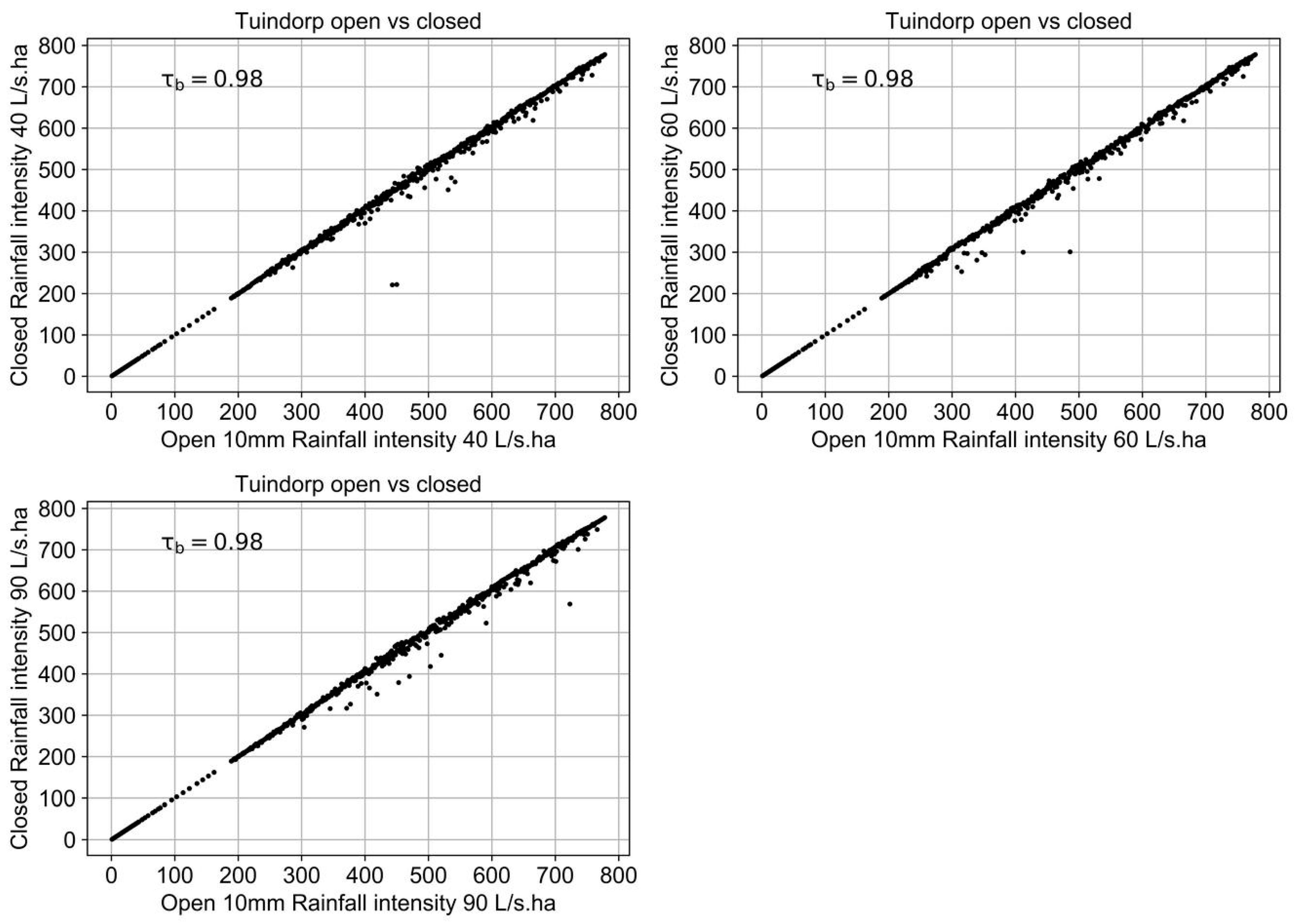
Figure 7 shows the results of the comparison of the degree of criticality based on the HMM for the Tuindorp catchment. In one situation, the conduit is completely blocked, in the other situation the diameter is reduced to 10 mm.
Figure 7 shows that the results are not exactly the same but are similar to each other and the τ
b value is 0.98. The degree of criticality is ranked from most important (1) to least important (778). If the dots are at situated at one line, the ranking of the conduits in both methods is the same. The more the points deviate from the line, the greater the difference between the two methods.
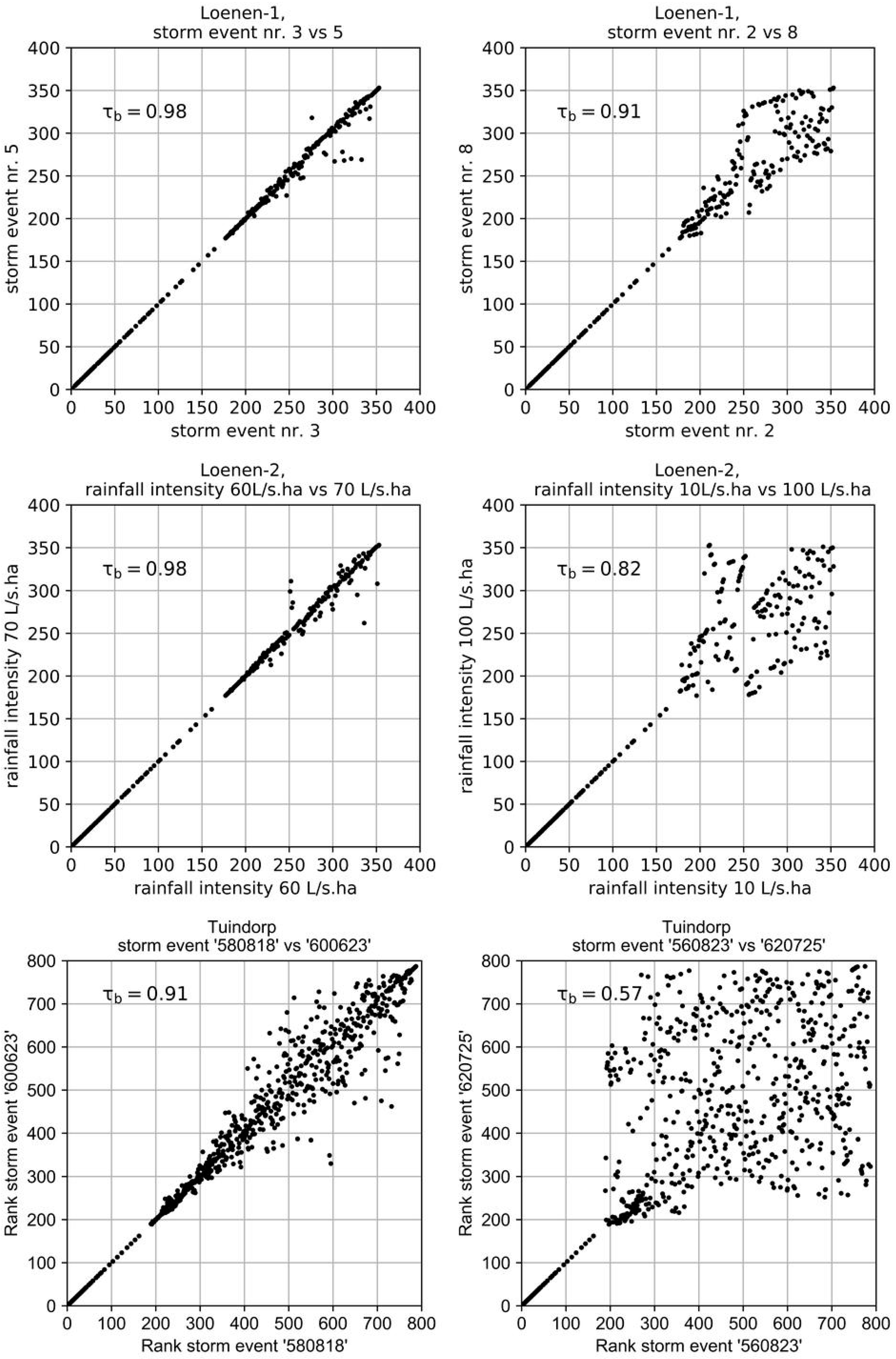
3.2. The Degree of Criticality Based on Hydrodynamic Model Method
With the hydrodynamic model method (HMM), the criticality of the conduits is determined for different storm events. For the three types of storm events (stationary, dynamic, series) the degree of criticality of the conduits is per two events plotted against each other and τb is determined. If the degree of criticality is independent of the storm event the τb value is 1.
Table 2,
Table 3 and
Table 4 show some of the results (see
Appendix A Figure A1 and
Table A1,
Table A2,
Table A3,
Table A4 and
Table A5 for more results). The tables show that the type of storm event does affect the degree of criticality of the conduit. If the differences in maximum rainfall intensity and/or shape between the storm events are limited τ
b ≈ 1 and the degree of criticality of the individual elements is almost the same. If the differences between the storm events become larger τ
b drops below 0.6 (see
Appendix A Table A1,
Table A2,
Table A3,
Table A4 and
Table A5) and the degree of criticality of the individual elements changes. This can be both an increase and a decrease of the degree of criticality.
The removal of a conduit of the Loenen network results in 176 cases in one or more nodes that are no longer connected to a combined sewer overflow. For Tuindorp this is the case for 188 conduits. These conduits are ranked based on the runoff surface that can no longer drain to a CSO. The degree of criticality of these conduits is therefore storm independent.
As the dynamics of the hydraulic load is an important factor in the distribution of water flows in networks, it is not feasible to determine a single value for the criticality of an element in a network when applying the HMM method. The results also show that the degree of criticality varies both for conduits with a lower and higher degree of criticality. This is observed for stationary storm events as well for dynamic design storm events and observed storm events. The effect is present in both sewer systems.
3.3. Comparison Degree of Criticality Based on a Hydrodynamic Model and on the Graph Theory
The degree of criticality based on the graph theory method (GTM) is compared with the outcomes of the hydrodynamic model method (HMM) in terms of the Kendalls’ τ
b. For the GTM, the costs of the conduits are decisive for the outcomes. As described in
Section 2.5.1 the costs of the conduits depend on the parameters discharge, water level and crest difference. The impact of the value of the parameters is described in more detail in
Section 4.1.
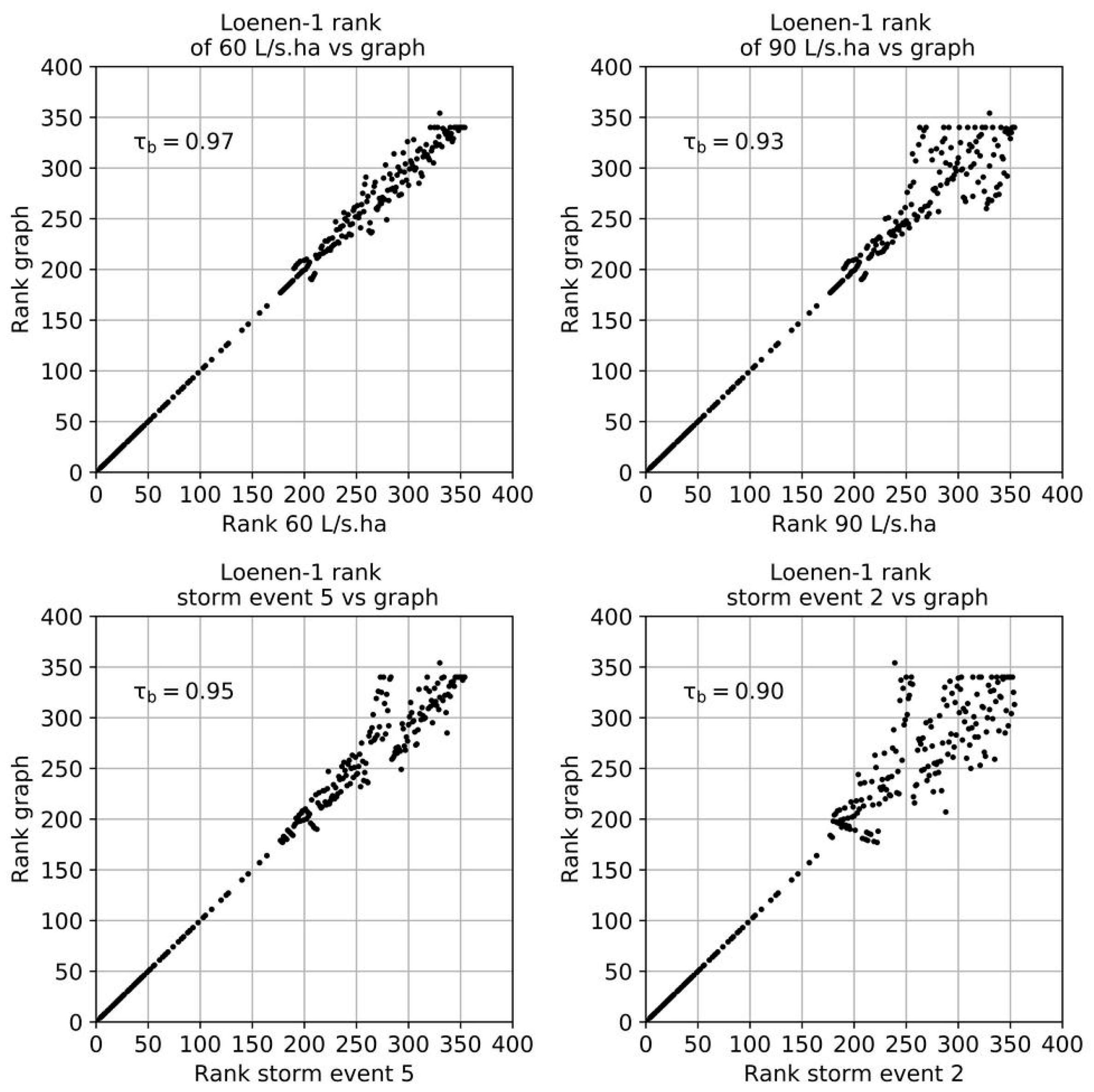
Figure 8 shows the results of the comparison with the dynamic and stationary storm events with the highest and lowest τ
b for Loenen-1. τ
b varies between 0.97–0.90. That implies that for all combinations of parameters and storm events there is a strong relation in the outcomes of the HMM and the GTM.
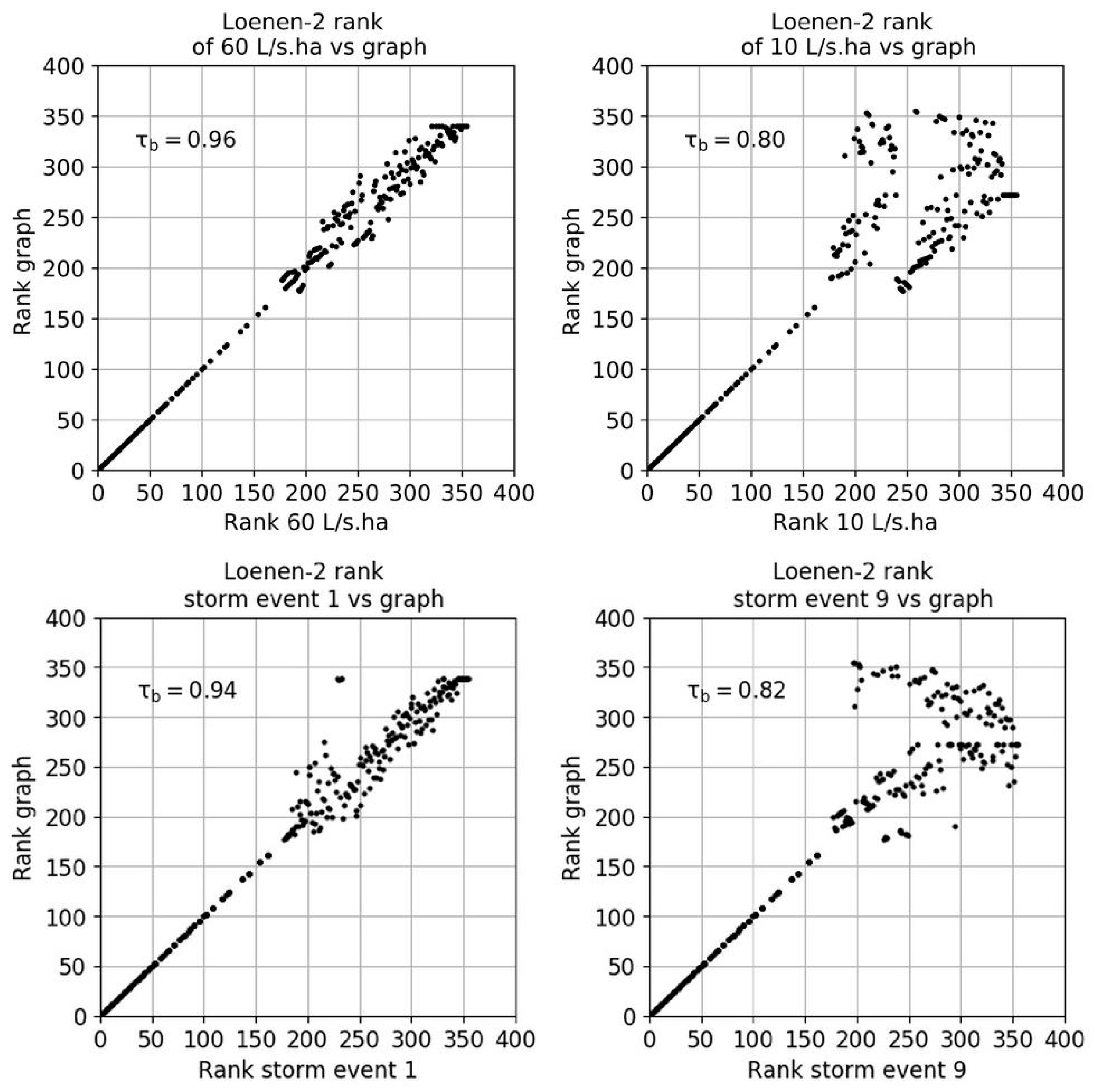
The Loenen-2 network is more complex than the Loenen-1 network because of the additional CSO. For Loenen-2, τ
b varies between 0.80–0.96: that is 0.01–0.1 less than the τ
b of Loenen-1. A τ
b of 0.80–0.96 implies that also for Loenen-2 there is a strong relation in the outcomes of the HMM and the GTM.
Figure 9 shows the results of the comparison with the dynamic and stationary storm events with the highest and lowest τ
b.
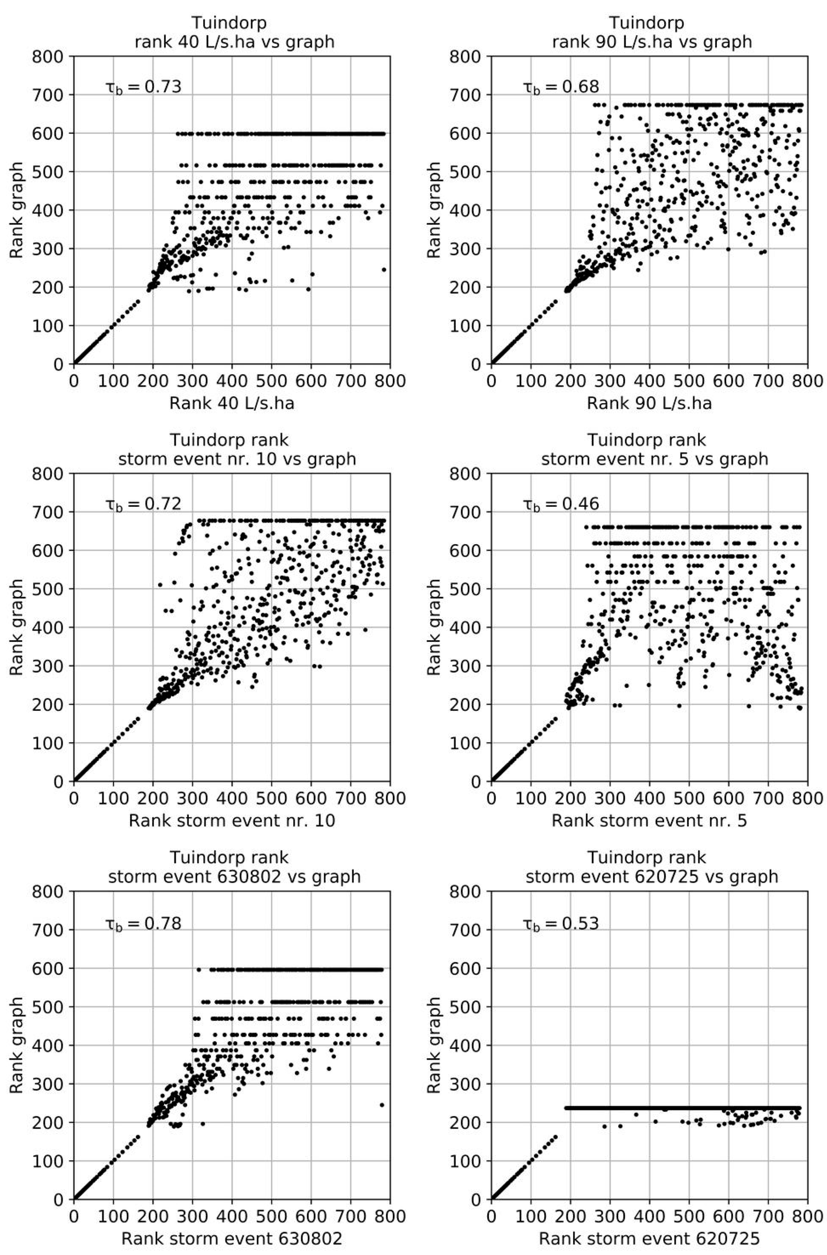
Figure 10 shows the results for the Tuindorp case. The Tuindorp network is more complex than the Loenen network because the number of conduits and CSO structures is more than twice as large. The Kendalls’ τ
b between the results of the hydraulic model and the graph method are less than for the Loenen cases. The Kendalls’ τ
b varies between 0.46–0.78. Although the Kendalls’ τ
b is reduced, it is still possible to identify the 250–300 (30–40%) most important conduits with the GTM.
4. Discussion
An analysis is made of the causes of the differences between the HMM and the GTM as presented before. As explained in
Section 3.2, a major difference between the methods discussed is the fact that the HMM is not storm independent.
An important cause of the differences in results between the HMM and the GTM is that a fixed discharge is used for all conduits in the GTM. The GTM does not take into account that in case of a blockage the discharge in the other conduits increase. An increase in discharge causes a higher head loss in the HMM. This is clearly observed in case of parallel links. In the HMM, blockage of one of the parallel links results in an increase of the water levels, along with an increased degree of criticality. In the same situation the GTM shows almost no increase in costs when one of the parallel conduits is blocked because the costs of both parallel conduits are almost the same and are not adjusted for the hydraulic processes taking place.
The same effect is visible when two CSOs are connected by a conduit with a relatively large hydraulic capacity. When a conduit close to the CSO is blocked, the water either has to flow to the other CSO or flooding occurs. In the HMM, this causes an increase of the water levels at many manholes because the discharge in the conduits to the not blocked CSO increases. So the conduit is ranked as important. The additional costs in the GTM are limited when the hydraulic capacity of the conduit between the two CSO is large so the conduit is not ranked as important.
A second cause of the difference in outcomes is the fact that the HMM makes distinctions between flooding and increases in water level. The GTM only calculates the increase in costs in the case of a blocked pipe. An increase in costs is weighted equally everywhere. In the HMM, the same increase in water level is marked as more important when the increase results in flooding. The intensity and the shape of the storm event influence this aspect.
For the Tuindorp catchment, the dynamic storm events 5 and 6 have a lower correlation than the other storm events (
Figure 11,
Figure 12 and
Figure 13). Storm events 5 and 6 have a return period of 1 year. Storm event 5 is an event with the peak intensity at the beginning of the storm event and storm event 6 has peak intensity at the end. These are storm events with maximum water levels for the fully operational sewer system between 0.1–0.25 cm below ground level in the most critical parts of the network while in the less critical parts of the network the maximum water level remains deeper below ground level. A diameter reduction of a conduit in a less critical part of the network that causes a larger increase in water level than a diameter reduction in a critical part is ranked as less important if the diameter reduction in the lower part causes a flooding.
The network of Tuindorp clearly shows the influence of the characteristics of the storm event on the ranking based on the hydraulic models. In case of storm events with high rainfall intensity at the start of the event, conduits in the surrounding of the pumping station are ranked as more important because the water degree of the sewer system influences the ponded nodes. When the peak intensity is at the end of the event the system is already completely filled and the discharge via the pumping station is no longer relevant.
A third cause of difference is the variation in ground level in combination with the network layout. In the Loenen catchment a conduit is situated on a slope. There are two paths to a CSO and the length of the two paths is different. This results in a relative large difference in costs. If the shortest route is blocked the additional costs for the GTM are relatively high and the degree of criticality is relative high. For the HMM the longer path results in an increase of water levels at only one node and the degree of criticality is relative low.
4.1. Sensitivity of Parameters in the Graph Methodology
The costs of the conduits depend on two variables; discharge and water level. The difference in crest levels of combined overflow structures is a third variable for networks with more than one CSO. The discharge influences the dynamic part of the costs of the conduits. If a discharge of 0 m3/s is used, the dynamic part of the costs of the conduits is zero. With an increasing discharge, the relative importance of the dynamic part of the costs of the conduits increases. The ratio of the dynamic part of the costs between the conduits remains the same because for all conduits the same discharge is used.
The water level influences the static parts of the conduit costs. The conduits with both invert levels below the water level have no static costs. If the water level varies between the lowest and highest invert level the static cost component decrease if the water level increase and vice versa.
The difference in crest levels of combined overflow structures determine the additional costs of the use of an overflow with a higher crest level as target node.
To determine the influence of these variables on the degree of criticality, these variables have been varied. The discharge has been varied between 0–0.2 m3/s, the water level between 0–1 m above the lowest crest level, the costs for the differences in crest level between 0–0.5 for the Tuindorp case and between 0–1 for the Loenen case. For each value the degree of criticality is determined. The outcomes of the graph method are compared with the outcomes of the hydraulic model. For the comparison of the degree of criticality the Kendall’s τb has been used.
4.1.1. Discharge
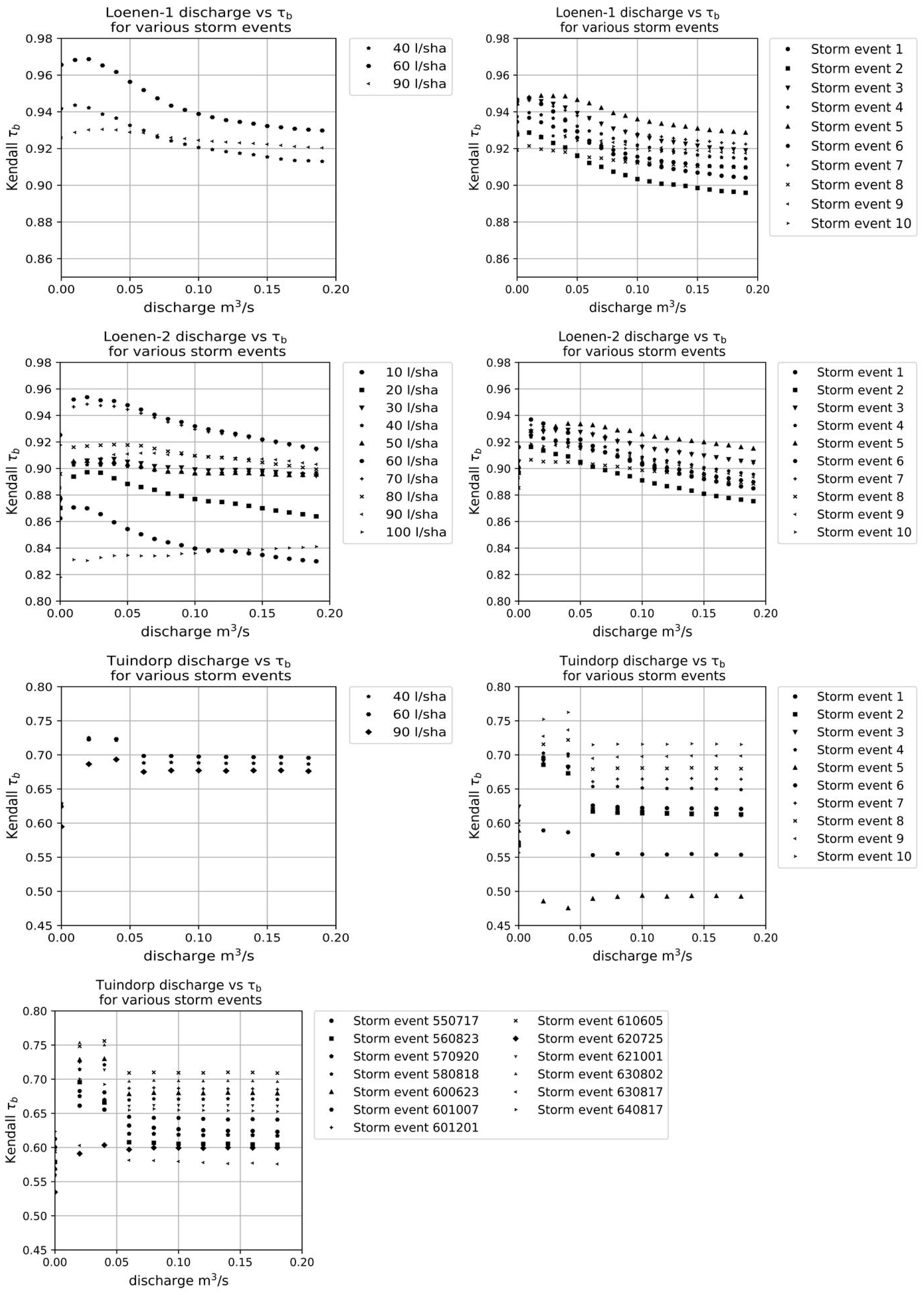
Figure 11 shows the results of the sensitivity analysis of the discharge of the results of the GTM. The graphs show that a discharge of 0.02 results in a maximum for τ
b. The variation in τ
b is limited to ≈0.05. τ
b is small if the discharge is 0, and after a peak around 0.02 m
3/s τ
b decreases with increasing discharge. As mentioned before, the discharge influences the dynamic costs. With a discharge of 0 m
3/s, the dynamic costs are ignored and with a higher discharge the dynamic costs become relative high in relation to the static costs. It is important that the dynamic costs have the same order of magnitude as the static costs.
Because Loenen is situated in a mildly sloped area, the static costs are more important than the dynamic costs. Due to the variation of the ground level, the height differences determine (in combination with the structure of the network) to an important extent the criticality of the conduits. The costs to overcome differences in altitude (static costs) are higher than the additional dynamic costs caused by smaller conduit diameters (dynamic costs).
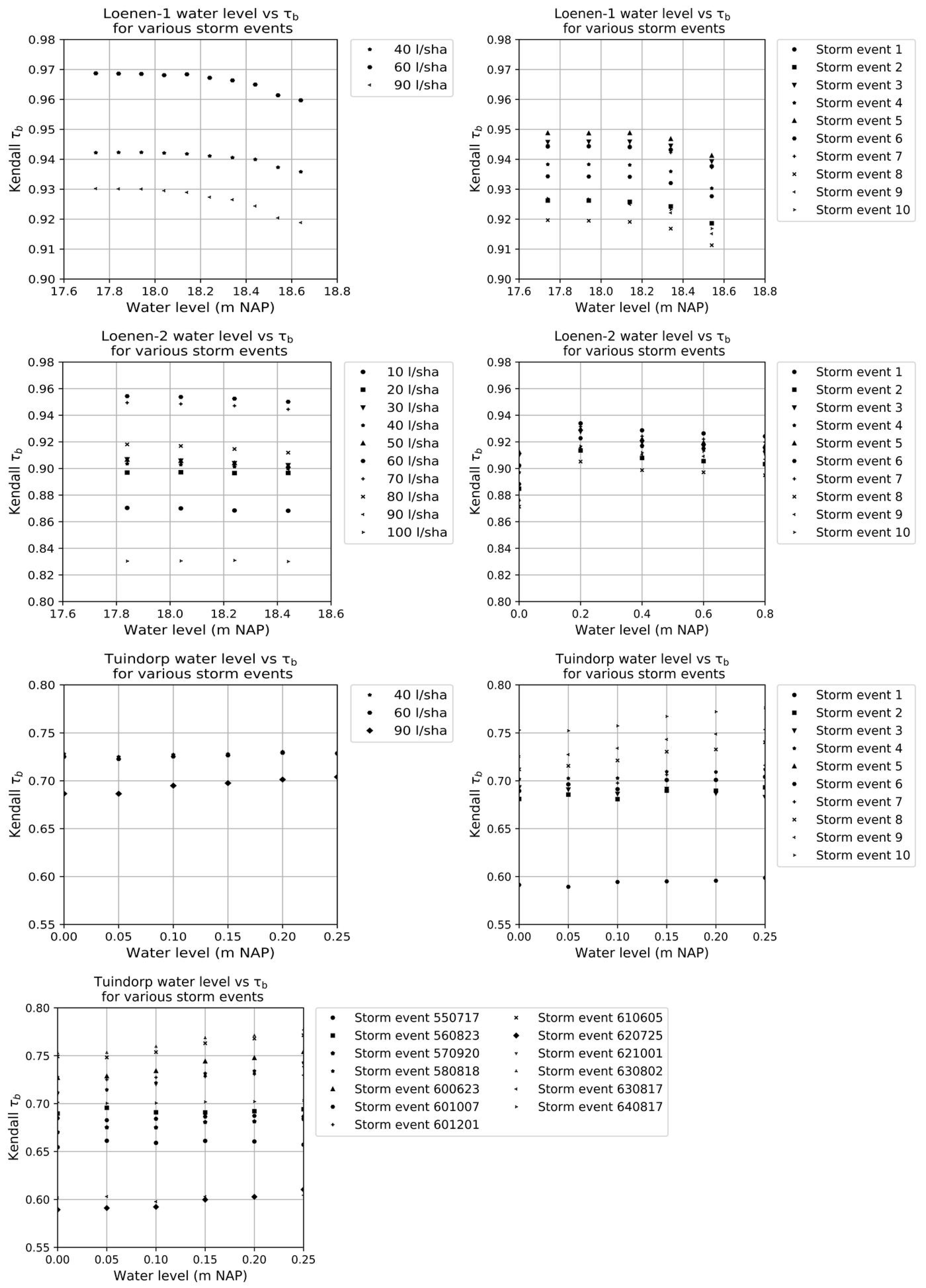
4.1.2. Water Level Sewer System
For Loenen-1 and Loenen-2, the effect of the water level is limited (see
Figure 12) because Loenen is situated in a mildly sloped area and a higher water level affects only a limited number of conduits. For Tuindorp, the effect of the water level is also limited because only less than 10% of the invert levels of the conduits are situated above the lowest weir. A water level equal to the lowest CSO or equal to the design level of the flow over the CSO (in The Netherlands 0.3 m) is a valid assumption.
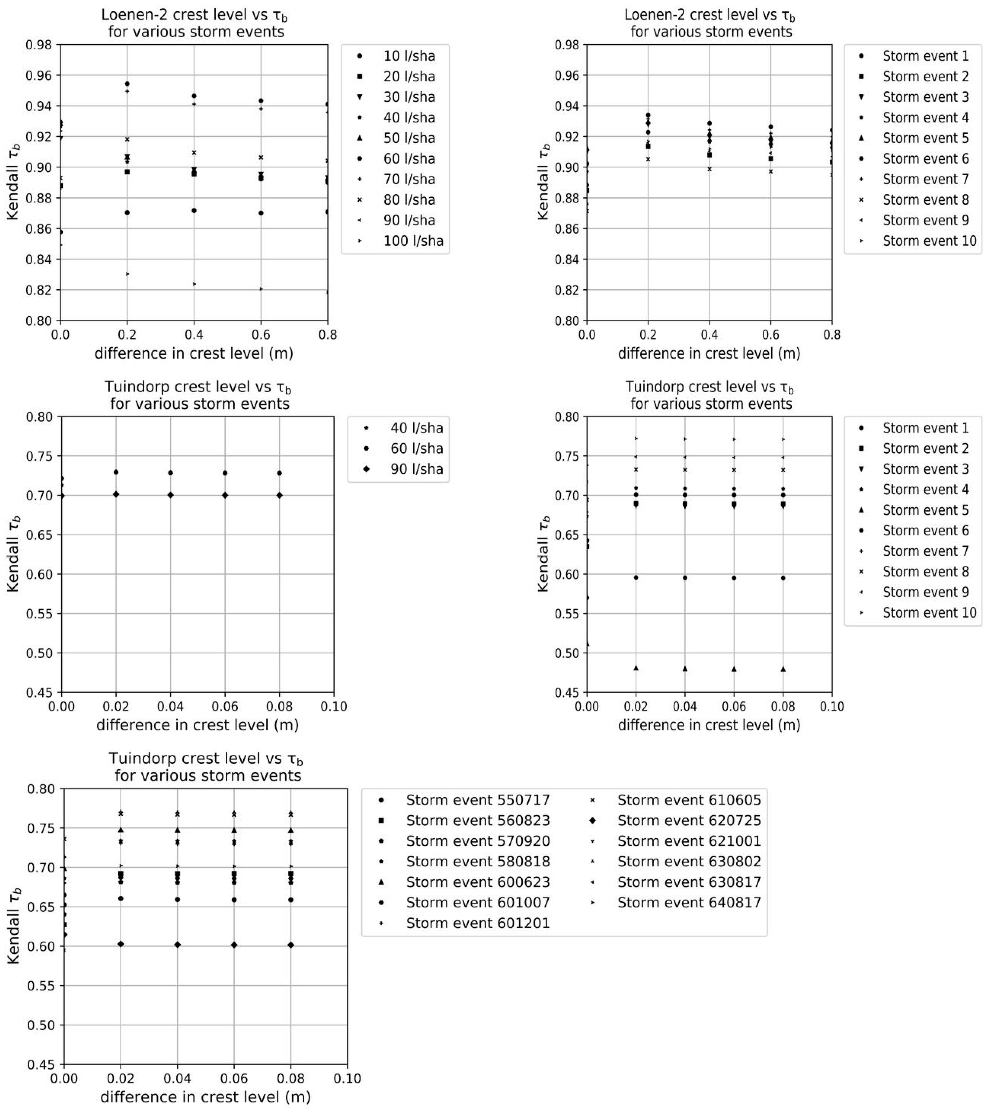
4.1.3. Difference in Crest Levels Sewer System
For the sewer systems with more than one CSO and with different crest levels, a small (<0.1) additional cost for the CSOs with a higher crest level have a positive effect on τ
b but the effect is limited (<0.05) (see
Figure 13). The degree of criticality can change strongly if another crest height is used. Conduits with a high degree of criticality can get a low degree of criticality when another difference in crest height is used and vice versa. This means that it is important to select the additional costs for overflows with different crest heights carefully in flat areas.
The additional costs for higher crest levels must be in the same order of magnitude as the dynamic costs. So, if a low discharge is used the additional costs also must be low and if a higher discharge is used the additional costs can be higher.
4.2. Performance
Table 5 shows the performance of the hydraulic model and the graph theory methodology. All calculations are made on the same computer. The table shows that the GTM methodology based on the graph theory is a few hundred to a few thousand times faster than the HMM method based on the hydraulic models if one storm event is used in the HMM.
4.3. Criticality of the Conduits
Figure 14 and
Figure 15 show the results of the criticality of the conduits for Loenen and Tuindorp based on the GTM. The figures show that, as expected, the conduits that cause a part of the network to be disconnected when these conduits are blocked are classified as important. Other important conduits are the conduits in the direction of the combined overflow structures. For Loenen there is a clear difference between the situations with 1 and 2 CSOs (Loenen-1 and Loenen-2). This is also visible in the results of the hydraulic model. For Tuindorp, the links between the CSOs are linked as moderate important by the GTM. These conduits are ranked as more important based on the HMM.
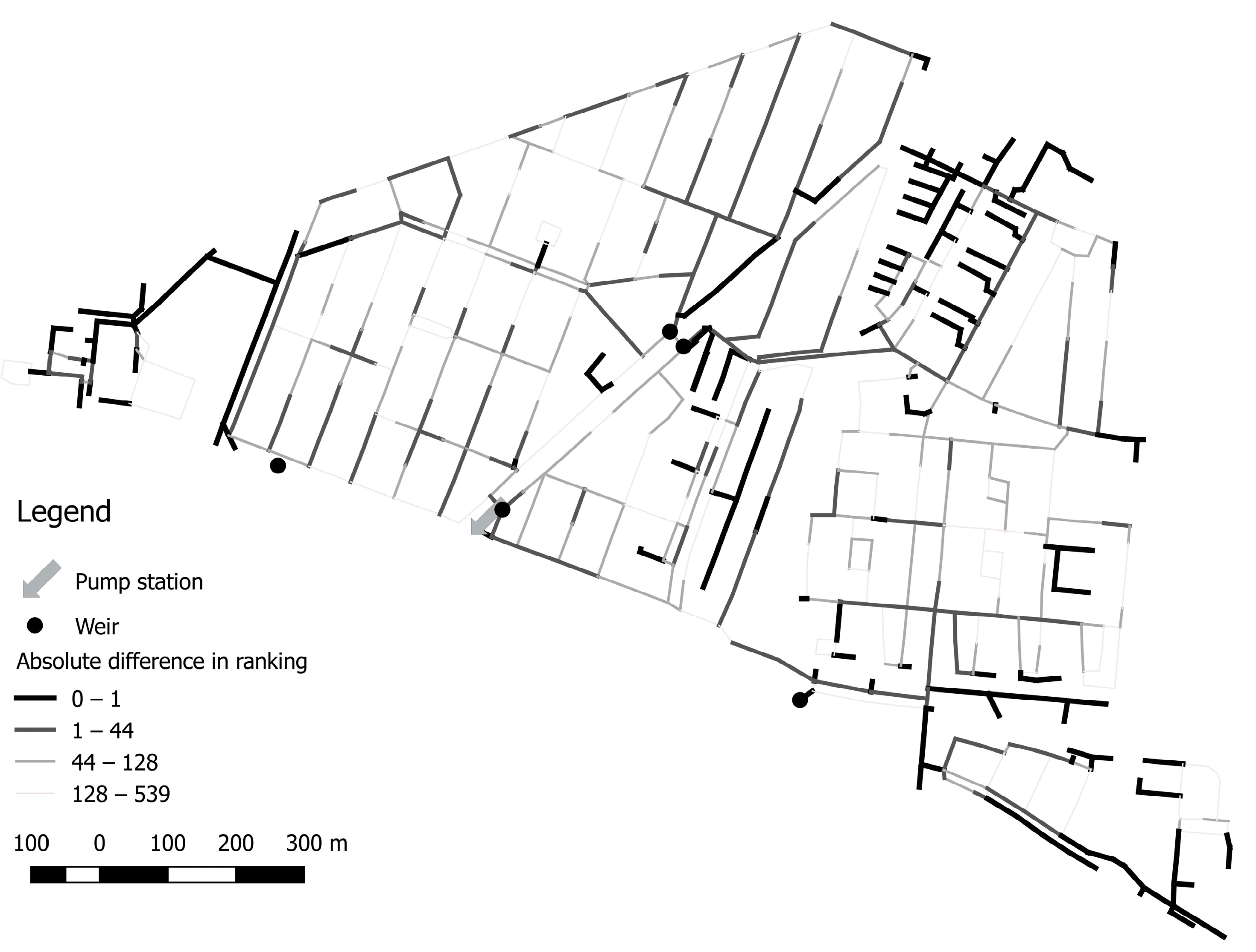
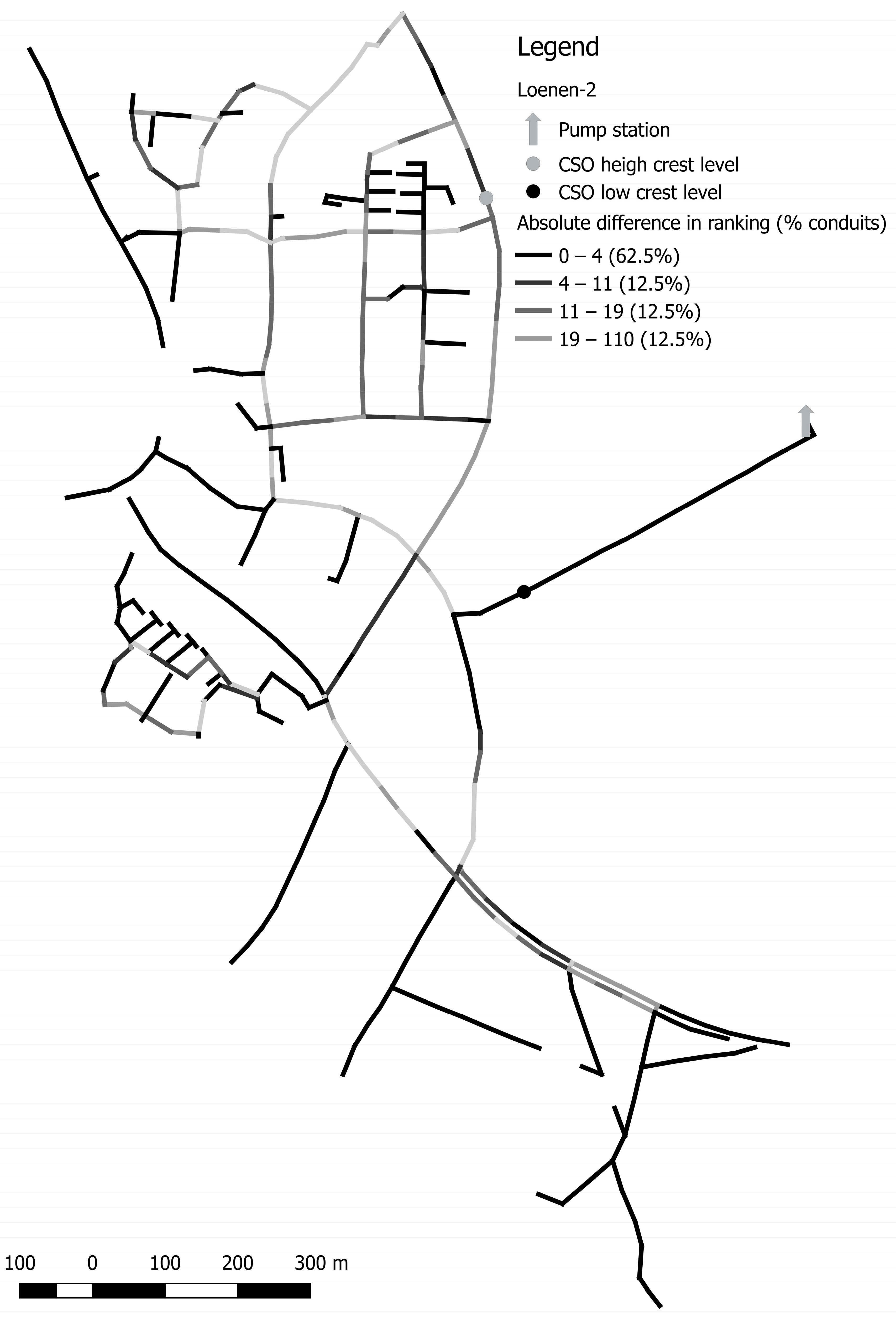
Figure 16 and
Figure 17 show the results of the comparison between the results of the HMM and the GTM. The darker the line the smaller the difference in criticality rank between the two methods.
5. Conclusions
In this paper, the graph theory method (GTM) is presented as a means to identify the most critical elements in a network with respect to malfunctioning of the system as a whole. The method is objective and independent of the type of storm event and requires limited computational effort. The degree of criticality of the conduits is compared with the hydrodynamic model method (HMM) (Achilles approach). There is a high correlation (Kendalls’ τb > 0.72) between GTM and HMM results.
The degree of criticality based on the hydrodynamic model method depends strongly on the used storm event. In the HMM the degree of criticality is determined by removing each conduit individually from the network. The links are ranked based on the total increase in flood volume and the increase of water level in the sewer system. The use of different storm events leads to a different ranking of the elements. Important elements become less important and vice versa. That means it is impossible to define one rank of the degree of criticality for different rainfall intensities by removing each conduit individually from the network.
The criticality for the partly branched mildly sloping catchment of Loenen has a stronger correlation with the results of a hydraulic model than the results of the looped, flat Tuindorp catchment. Nevertheless, it was shown that for both catchments it is possible to identify the 30–40% most critical conduits in a robust manner, compared to other methods as applied in practice.
For sewer systems, the degree of criticality based on the graph theory depends on three parameters: the discharge, the water level and the difference between crest levels of overflow structures. The outcomes of the GTM are not sensitive for the exact value of the variables as long as the variables have values that result in dynamic and static costs of the same order of magnitude. The importance of the dynamic part of the costs of the conduits is limited for sewer systems in (mildly) sloped areas where the overflow is situated in the lower part of the system.
Apart from the influence of the storm event, there are two main causes for the differences in the results of the degree of criticality based on the HMM and the GTM. The first cause is that, in the GTM, the same discharge is used for all conduits, also when one of the conduits in the system is blocked. The second cause is that, in the GTM, each increase in costs is equally important. In the HMM, an increase in water level that causes a flooding is weighted as more important than a comparable increase in water level without flooding.
The degree of criticality is an important input for risk-based asset management. The degree of criticality can be used to prioritize the required maintenance state of conduits and thus for the allocation of maintenance budgets. Before the GTM can be used in practice, additional research is required to determine the impact of the failures based on the characteristics of the area that is flooded.
Future research will focus on validation of the results for (larger) looped systems in flat areas, and the extension of the method for other network systems like gas and water supply networks, district heating networks and surface water systems for polders. Each kind of system/network has its own characteristics and the GTM has to be adjusted to fit to the system. Possible adjustments are the use of graph vs. digraph, removing edges (blockage) vs. adding demand nodes (leakage), fixed target nodes (weirs) vs. dynamic target nodes (leakages). Important characteristics that influence the elaboration of the GTM for other network types are summarized in
Table 6.
Preliminary results of an analysis of a water supply network indicate that the GTM also can be used to determine the criticality of elements in these networks [
33].

 ,
, 
