Article

Performance Assessment of General Circulation Model in Simulating Daily Precipitation and Temperature Using Multiple Gridded Datasets

1
School of Civil Engineering, Faculty of Engineering, Universiti Teknologi Malaysia (UTM), 81310 Johor Bahru, Malaysia
2
Faculty of Water Resource Management, Lasbela University of Agriculture Water and Marine Sciences (LUAWMS), 90150 Uthal, Balochistan, Pakistan
3
Department of Civil Engineering, Chungnam National University, Daejeon 34134, Korea
*
Author to whom correspondence should be addressed.
Water 2018, 10(12), 1793; https://doi.org/10.3390/w10121793
Submission received: 28 September 2018 / Revised: 29 November 2018 / Accepted: 4 December 2018 / Published: 6 December 2018
(This article belongs to the Section Hydrology)

Abstract

:
The performance of general circulation models (GCMs) in a region are generally assessed according to their capability to simulate historical temperature and precipitation of the region. The performance of 31 GCMs of the Coupled Model Intercomparison Project Phase 5 (CMIP5) is evaluated in this study to identify a suitable ensemble for daily maximum, minimum temperature and precipitation for Pakistan using multiple sets of gridded data, namely: Asian Precipitation–Highly-Resolved Observational Data Integration Towards Evaluation (APHRODITE), Berkeley Earth Surface Temperature (BEST), Princeton Global Meteorological Forcing (PGF) and Climate Prediction Centre (CPC) data. An entropy-based robust feature selection approach known as symmetrical uncertainty (SU) is used for the ranking of GCM. It is known from the results of this study that the spatial distribution of best-ranked GCMs varies for different sets of gridded data. The performance of GCMs is also found to vary for both temperatures and precipitation. The Commonwealth Scientific and Industrial Research Organization, Australia (CSIRO)-Mk3-6-0 and Max Planck Institute (MPI)-ESM-LR perform well for temperature while EC-Earth and MIROC5 perform well for precipitation. A trade-off is formulated to select the common GCMs for different climatic variables and gridded data sets, which identify six GCMs, namely: ACCESS1-3, CESM1-BGC, CMCC-CM, HadGEM2-CC, HadGEM2-ES and MIROC5 for the reliable projection of temperature and precipitation of Pakistan.

1. Introduction

Simulations of general circulation models (GCM) are generally used for the assessment of climate change. However, the GCM simulated climate is associated with large uncertainties due to model structure, parametrization, assumption, calibration processes and so on [1,2]. Therefore, all the GCMs cannot be directly used to project the future climate in certain regions. In general, a small group of GCMs is selected for a given region by excluding those which have no similarity to the climate in order to reduce the uncertainty associated with the GCMs [3,4,5,6].
Generally, GCMs are selected based on several approaches; first, the past performance-based approach which selects GCM based on its ability to replicate historical climate [7] and second, the envelope approach where GCMs are selected according to their agreement in the projections of the future climate [8]. The past performance evaluation method does not take account of the future projection of the climate while the envelope-based evaluation does not consider the GCM ability to replicate the past climate. Therefore, the third approach known as the hybrid approach, which combines the past-performance approach with the envelope method is often used. In this approach, the GCMs are screened based on their past performance. Then, the final set of GCMs are selected based on envelope approach [3]. However, when a whole pool of GCMs is considered for the selection of an ensemble, the past-performance approach is more realistic as the pool of GCMs covers the whole range of projections. Most of the previous studies also suggest that past performance evaluation is one of the most suitable approaches because the GCMs that are best in simulating the past climatic conditions are more likely to predict the future climate [9,10].
The past-performance of GCMs is usually assessed by comparing the GCM simulated climatic variables with the gridded climatic variables over a historical period. It is assumed that all gridded data used for this purpose represent the seasonal and spatial variability of the climate of the desired region. However, the performance of gridded climate data varies dramatically with space and time. This is mainly due to the type of interpolation technique, the quality of observed data and the spatial distribution of the gauges [11]. Additionally, the temporal variation in the number of observed data also affects the performance of gridded data over time. Therefore, the past performance assessment of GCMs based on single gridded data over a longer period may not be reliable.
Feature selection approaches are generally used for the selection of GCMs. The feature selection algorithm can be broadly classified into filter and wrapper. In the case of a filter approach, the GCMs are selected based on the underlying characteristics of the data using certain criteria such as correlation, mean error and so on. A wrapper approach uses a learning process to select a subset of features that have a higher capability to predict the independent variable. In the case of a filter approach, each feature is considered individually without consideration of correlation among the features. For GCM selection, it is not necessary to consider the relation between GCM simulations or predictive capability of GCMs. Therefore, filters are generally used for the selection of GCMs [12].
Various attempts have been conducted to determine the performance of GCMs in respect to gridded data using different types of filters which include weighted skill score [13,14], clustering hierarchy approach [15,16], spectral analysis [17], Bayesian weighting [18], different performance indicators [19,20] and so on. Besides, various statistical indicators have been used for GCM evaluation, ranking and selection [21,22,23,24,25,26,27]. The performance matrices are mostly evaluated on the basis of the mean state of the climatic condition where temporal variability such as trends or seasonal variability of the climate is not given full attention [28].
In recent years, one of the widely used algorithms for the variable selection is the symmetrical uncertainty (SU) algorithm. This filter-based tool [29] selects variables in an unbiased and reliable manner. The SU can track the similarity and dissimilarity between the time series of GCM simulation for historical period and observed climate variable and select the GCMs based on their ability to simulate observed climate variable. The major advantage of SU is that its performance does not depend on the underlying distribution and different conditional dependencies of data. It provides a general aspect of the association between the independent and the dependent variables. Therefore, it can be used to avoid multiple statistical metrics for performance assessment.
The objective of this study is to evaluate the capability of 31 CMIP5 GCMs in reconstructing of temperature and precipitation from different gridded data using SU to identify the most suitable ensemble of GCMs for the reliable climate projection. This study is applied to the case of Pakistan where a diverse climate with large spatial and seasonal variability exist. The ensemble of GCMs selected in this study can be used for reliable projection of climate and mitigation planning for Pakistan which is highly vulnerable to climate change.

2. Materials and Methods

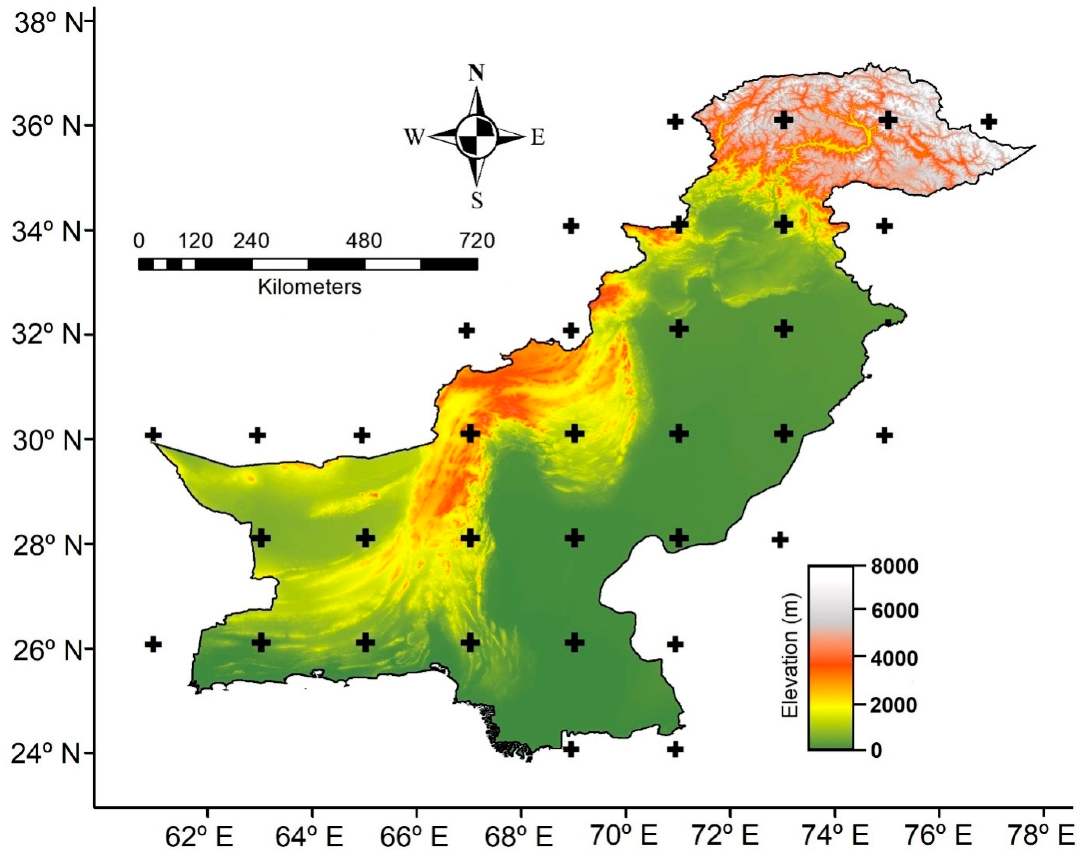
2.1. Geography and Climate of Pakistan

Pakistan (latitudes 24°00′ N–37°30′ N and longitudes 61° E–78° E) covers an area of 796,095 km2 showing a predominantly arid to semi-arid climate [30]. The topography of Pakistan significantly varies from a high and elevated region in the north to the coastal flat plains in the south (Figure 1), depending on which huge spatial and temporal variation in the climatic condition is observed. The precipitation also varies widely with less than 100 mm in the western and northwestern area and more than 1100 mm in the northeastern and northern part of the country. The precipitation is observed to increase from the arid southern coastal regions to the northern and northeastern region of the country. However, the major parts of the country have a precipitation less than 500 mm [31]. The south eastern parts of the country have the highest rainfall during summer (June–September) and least rainfall during winter (December–February), while the northern parts have the highest rainfall during winter and the lowest rainfall in summer. The maximum temperature is often above 50 °C in the south in May, while the minimum temperature is below −20 °C in the northern Himalaya and sub-Himalaya region in January [30].

2.2. Data and Sources

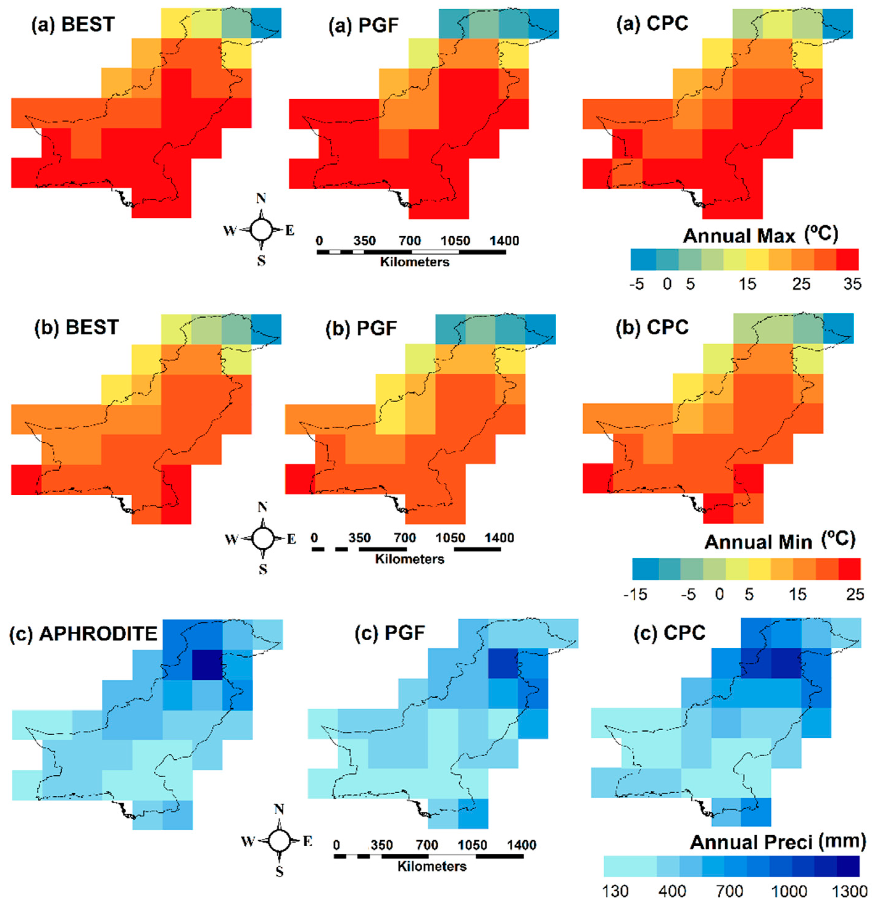
2.2.1. Gridded Datasets

Four gridded climate datasets are used in this study namely, Berkeley Earth Surface Temperature (BEST), Climate Prediction Centre (CPC), the Princeton Global Meteorological Forcing (PGF) and the Asian Precipitation Highly-Resolved Observational Data Integration Towards Evaluation of Water Resources (APHRODITE). The choice of these datasets is based on the availability of daily data for a longer period. The gridded data products which have the daily resolution are used for the assessment of the performance of GCMs with an expectation that GCMs selected based on those gridded data can be used to assess the changes in different climatic extremes which are estimated by daily gridded data and selected by GCMs. Assessment of the changes of climate extremes due to global warming is important for Pakistan as most of the studies revealed that major impact of climate change in the country will be due to the changes of climatic extremes such as heat waves, hot days, dry spells and heavy rainfall [32]. GCMs selected from daily rainfall and temperature gridded data is suitable to this purpose. The major characteristics and sources of the gridded data used in this study are summarized in Table 1. The BEST dataset is obtained from data from 36,866 stations [33], while the CPC dataset is developed using 30,000 stations data [34]. The PGF dataset is developed by merging the reanalysis data with observed data collected across the globe [35,36]. On the other hand, APHRODITE is developed using 5000 to 12,000 valid stations in the Monsoon Asian region (60° E–150° E longitude, 15° S–55° N latitude) [37,38,39].
Among the four gridded datasets maximum and minimum temperature data of BEST, CPC and PGF are used to assess the GCMs’ temperature, while the precipitation of CPC, PGF and APHRODITE are used for the assessment of GCMs’ precipitation. The annual mean maximum, minimum and precipitation for each dataset are presented in Figure 2. The selected data products are available in different spatial resolution range from 0.25 to 1°. The gridded datasets are regridded to a common spatial resolution of 2° × 2° to be in accord with the agreed resolution of the GCM. The placement of these grid points across the study area is shown in Figure 1. Grid average technique is used to upscale the gridded data into the coarse resolution. In this approach, temperature and precipitation data of all the grids within each 2° × 2° domain are averaged to convert the higher resolution data to lower resolution.

2.2.2. Coupled Model Intercomparison Project Phase 5 (CMIP5) General Circulation Model (GCM) Datasets

A total of 31 CMIP5 GCM simulations are used in this study. The name, modeling center and resolution of the GCMs used in the study are given in Table 2. The GCM simulations are downloaded from the Inter-governmental Panel on Climate Change (IPCC) portal [44]. The GCMs are selected on the basis of the availability of daily simulation for two representative concentration pathways (RCP) scenarios, RCP4.5 and RCP8.5. The RCP4.5 is an intermediate pathway scenario which shows a good agreement with the latest policy of lower greenhouse gas emission by the global community. Therefore, it is often considered as a very-good-case scenario in the context of recent policy directions [45]. On the other hand, RCP 8.5 is the business-as-usual scenario which provides the possible highest impact on climate change. Therefore, RCP 4.5 and RCP 8.5 were selected as these two scenarios can provide a possible complete range of impact. The GCMs are available in different resolutions. Therefore, all selected CMIP5 temperature and precipitation simulations are regridded into the common 2° × 2° grid for fair comparison using bilinear interpolation technique. This technique uses a minimum of four points from the domain and nearby areas to generate point output from each GCM at each grid point and thus provides a smooth interpolation. It is widely used for regridding of GCMs for comparison [4].

3. Methodology

3.1. Procedure

Temporal alignment does not exist between the daily simulation of GCMs and observed data. However, it is expected that GCMs are able to characterize the wet and dry seasons and warm and cold seasons reasonably well. Therefore, the daily gridded datasets are converted to monthly scale and the association of GCM data with gridded data is compared at a monthly scale to evaluate the performance of GCMs. The gridded data products which have daily simulations are used for the assessment of the performance of GCMs in order to facilitate the changes in different climatic extremes. The procedure for the evaluation of GCMs based on their historical simulation of temperature and precipitation is outlined below:
(1)
The GCMs are evaluated and ranked using SU at each grid point (total 36 grid points at 2° × 2° resolution to cover whole Pakistan, Figure 1) according to their capability to replicate gridded temperature and precipitation data for the period 1979–2005.
(2)
The GCMs are ranked based on their positions at different grid points using a weighting technique, where more weight is given to GCMs which archive a higher rank in most of the grid points. A separate list of rank is prepared for each climatic variable (maximum and minimum temperature and precipitation) and each gridded dataset.
(3)
The common GCMs appeared above the 50-th percentile of all GCMs in each list are identified as the most appropriate ensemble for the projection of temperature and precipitation of Pakistan.
The daily mean temperature can be used for the selection of GCMs instead of selecting GCMs separately for maximum and minimum temperature. For the projection of extremes, better simulation of minimum and maximum temperature instead of mean temperature is required. However, better simulation mean the temperature does not guarantee a better simulation of maximum and minimum temperature. Therefore, GCMs are selected in this study based on both maximum and minimum temperature. The ranking of GCMs at each grid point using SU and the ranking of GCMs for whole of Pakistan considering the SU rank at each grid points using a weighting technique are elaborated in the following sections.

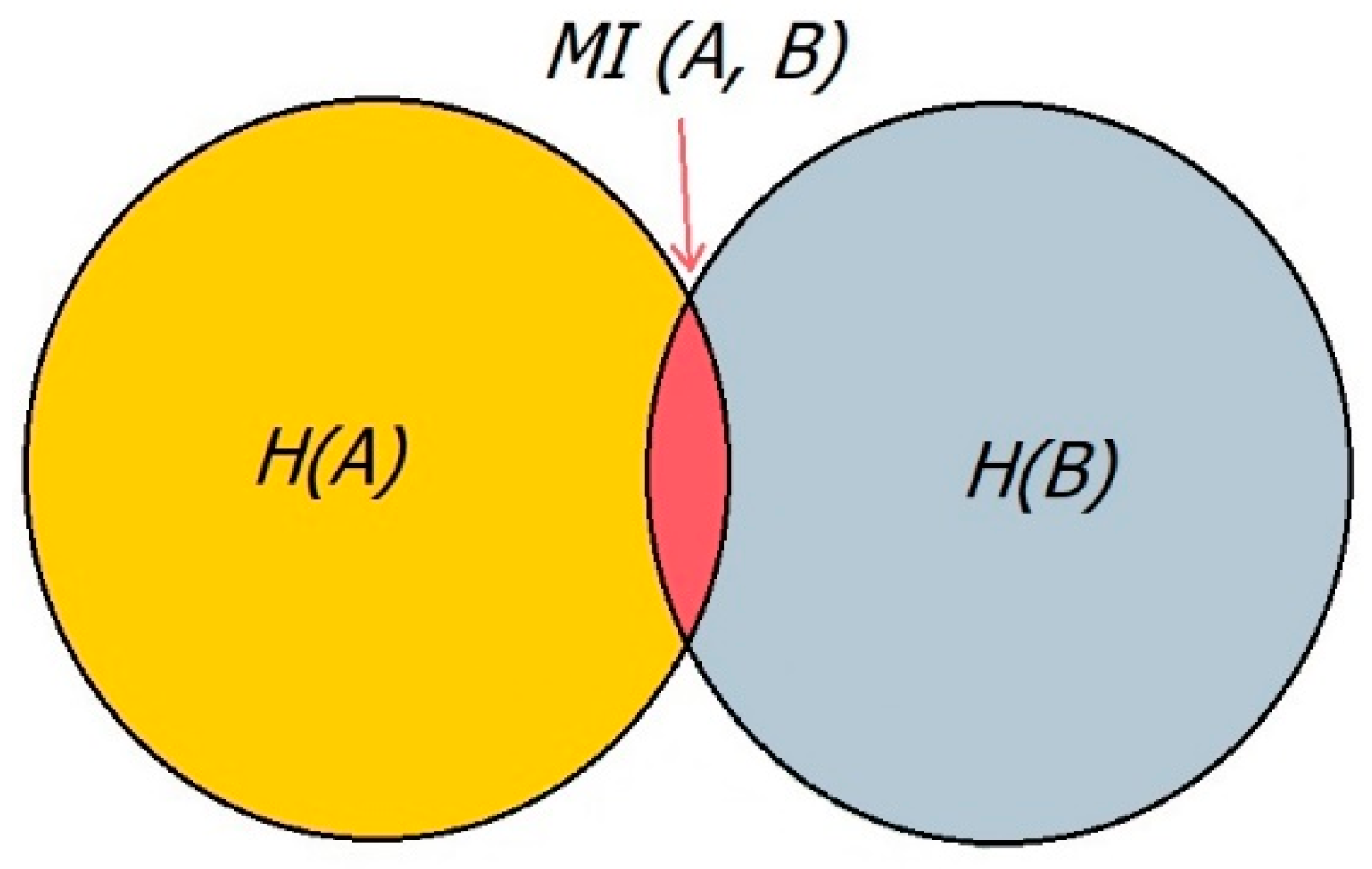
3.2. Symmetric Uncertainty (SU)

It is expected that GCMs have a capability to replicate the annual and seasonal variations of observed rainfall and temperature for the historical period. SU is a filtering approach based on information theory which can be used to assess the similarity between two time series [46]. In this study, SU is used to measure the similarity between the time series of gridded data and GCMs historical simulation [4,5]. For example, the monthly rainfall time series of the gridded data product is compared with result of GCMs at each grid point to assess the capability of the GCMs to replicate rainfall at each grid point.
SU uses the concept of mutual information (MI) to assess the association between two variables as shown in Figure 3. MI estimates the amount of information common between two variables. Let A and B be gridded rainfall and GCMs historical rainfall simulation at a grid point. If p(A) and p(B) are the probability density functions and p(A, B) is the joint probability density function of A and B, then MI between A and B is [47,48],
M I ( A , B ) = p ( A , B )   l o g p ( A , B ) p ( A ) . p ( B )
MI estimates common information between two variables as the difference between the sum of the entropies and their joint entropy:
M I ( A , B ) = H ( A ) H ( A , B )
where, H(A) and H(A, B) denotes Shannon’s entropy of A and the joint entropy of A and B, respectively. The MI estimated using Equation (1) indicates the amount of mutual information between gridded rainfall and GCMs historical rainfall simulation have. If the variables are independent to each other, the MI is zero while a higher value of MI indicates the GCMs simulated rainfall has higher similarity with the gridded rainfall.
The MI is biased toward the variable having higher values. This can be overcome using SU where the estimated MI is divided by the total entropies of GCMs simulation (B) and gridded data (A):
S U ( A , B ) = 2 M I ( A , B ) H ( A ) + H ( B )
SU value 1 means a complete agreement between gridded data and GCMs simulation, while 0 indicates no agreement [49]. Details of the selection of GCMs based on SU are found in [4,5].

3.3. Ranking of GCMs using Weighting Method

SU provides a ranking of GCMs at each grid point. A simple multi-criteria decision-making approach is used in this study for the selection of GCMs for the whole study area based on the ranking of GCMs obtained at different grid points. If a GCM achieved 1st, 2nd, 3rd, 4th and 5th ranks at X1, X2, X3, X4 and X5 number of grid points, the GCMs are assigned a weighted score:
s = X 1   ( 1 / 1 ) + X 2   ( 1 / 2 ) + X 3   ( 1 / 3 ) + X 4   ( 1 / 4 ) + X 5   ( 1 / 5 )
The GCMs rank more than 5th at a grid point are not considered because it is considered that they are not fully capable to simulate temperature or precipitation at that grid point.

4. Results

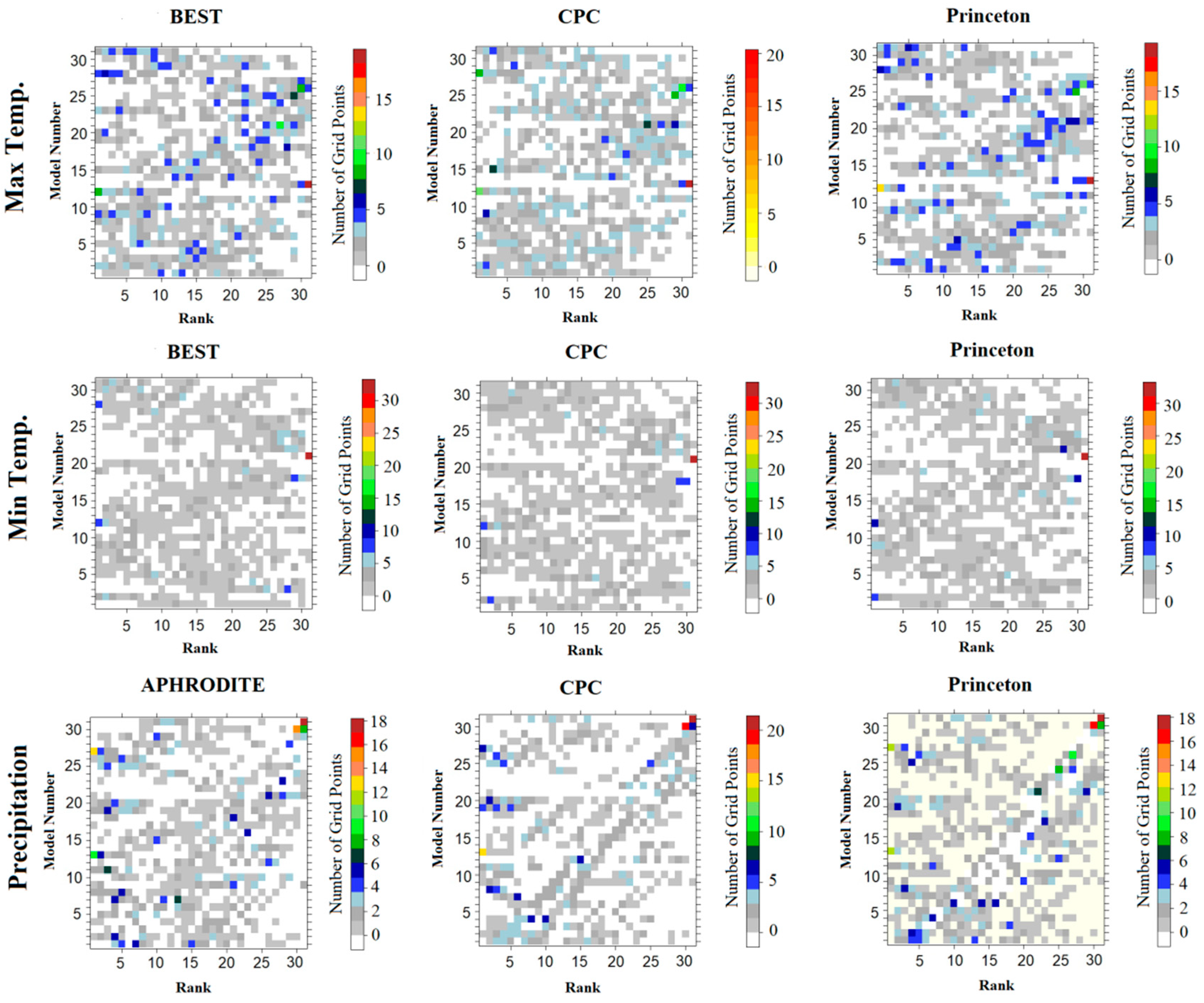
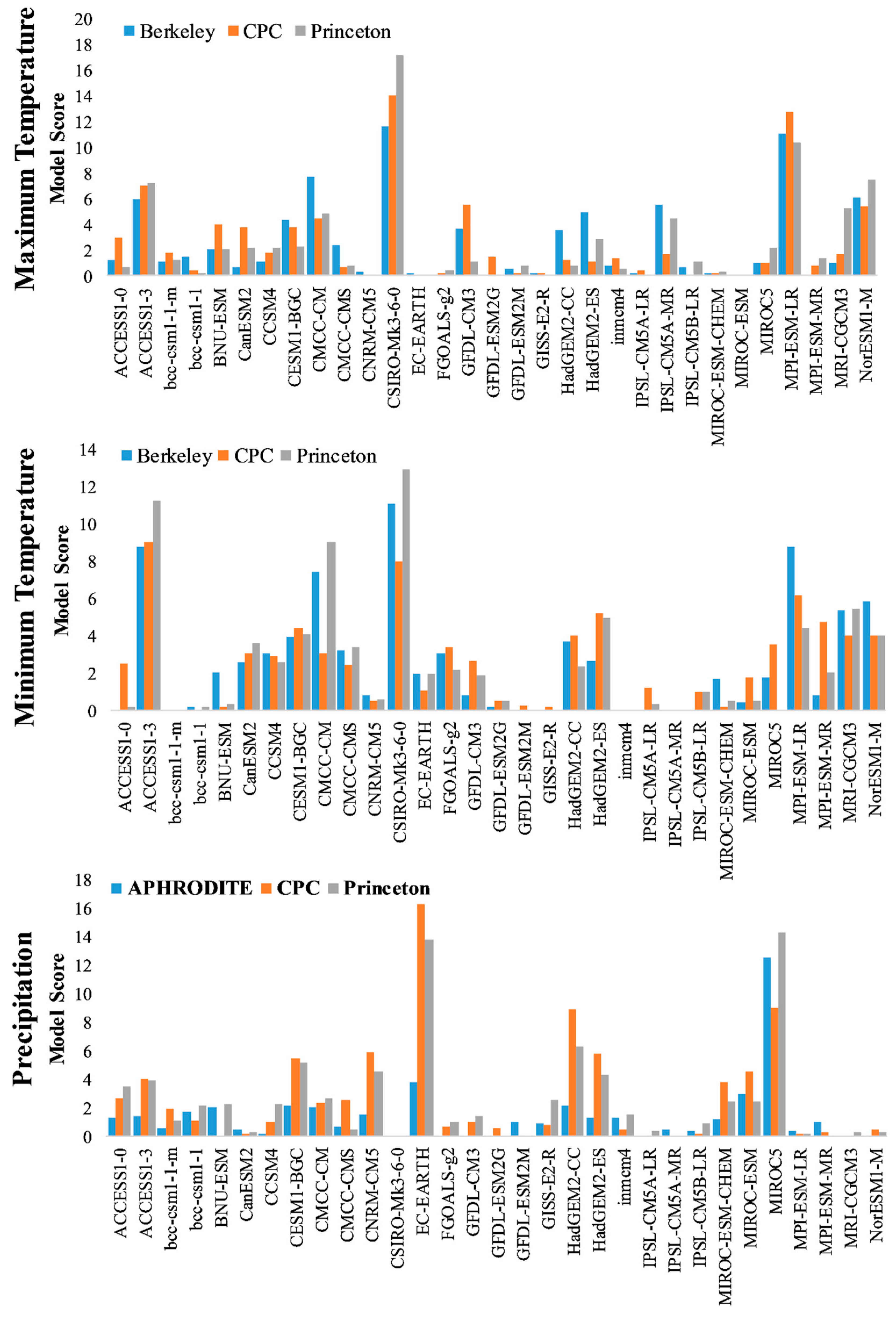
4.1. Ranking of GCMs

The ranking of GCMs in respect of their capability to replicate maximum and minimum temperature of BEST, CPC and PGF and precipitation of APHRODITE, CPC and PGF obtained by SU are shown in Figure 4 (heatmap plots). The x-axis and y-axis of the plot represent GCMs and their ranks, respectively. The number in the y-axis corresponds to GCM number which can be found in Table 2. For example, GCM number 1 represents ACCESS1-0, number 2 represents ACCESS1-3 and so on as seen in Table 1. The color ramp in the plot indicates the number of grid points. For example, CSIRO-Mk3-6-0 (GCM 12) achieved rank 1 at 11 grid points, EC-EARTH (GCM 13) is not ranked top at any grid point.
Different GCMs are ranked top at a different number of grid points (Figure 4). However, there is a consistency among the plots which indicate a similar ranking of GCMs at each grid points obtained from different gridded datasets. For example, CSIRO-Mk3-6-0 (GCM 12) is found to be best at 11 grid points for CPC and BEST, while it is found best at 12 grid points for PGF. The MPI-ESM-LR (GCM 28) is found best at 6 to 8 grid points for different gridded datasets. Overall, the BEST and CPC show better similarity in GCM ranks compared to PGF.
The similar consistency is observed in the case of minimum temperature. BEST and CPC produce similar rankings of GCMs in the case of minimum temperature. The GCM ranks using PGF is also found very close to that obtained by BEST and CPC. In the case of precipitation, better similarity is observed in the case of APHRODITE and PGF. A slight variation in the ranking is observed in the CPC. It is known from the results that rankings of GCMs vary when different gridded datasets are used although the intensity of variation is not significantly high.

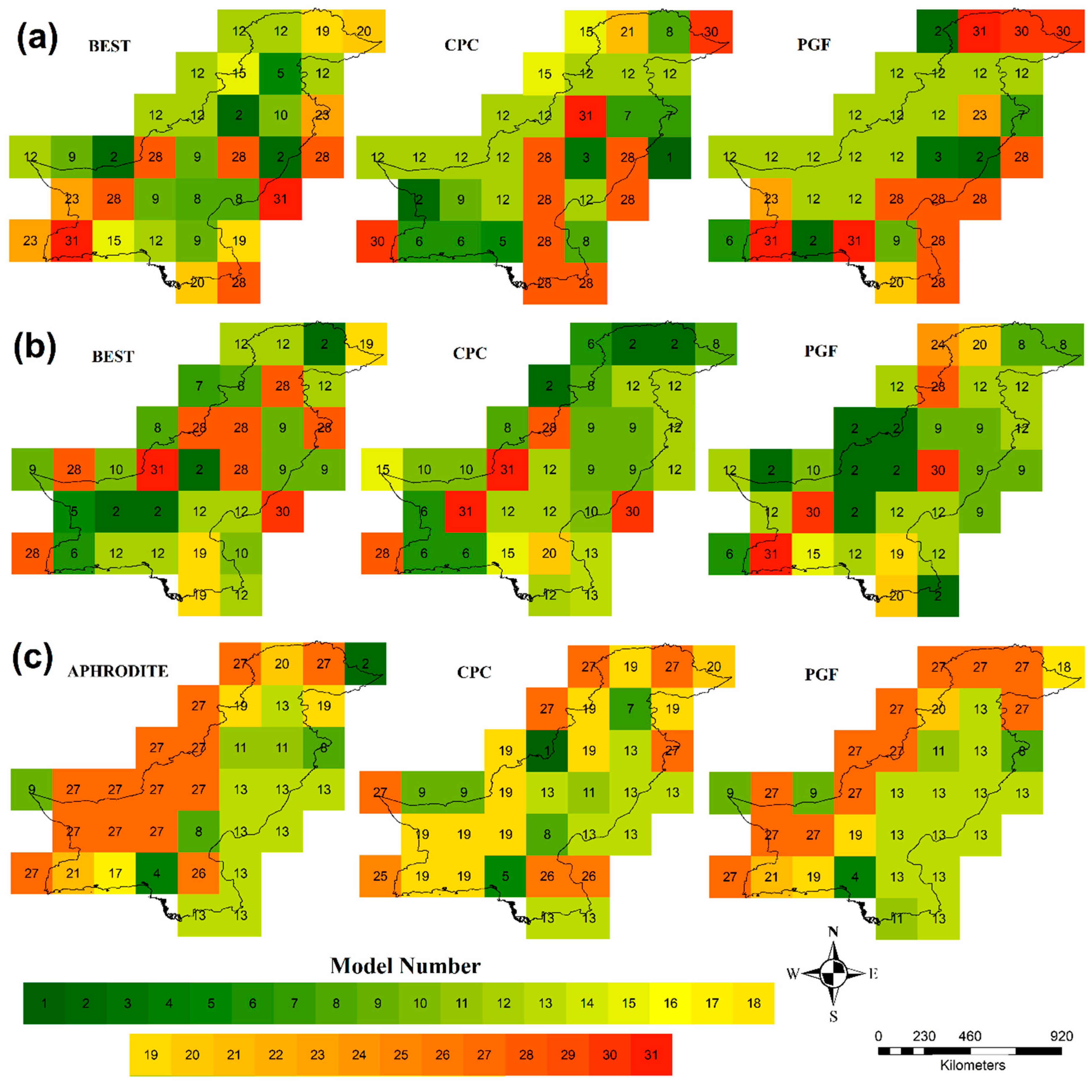
4.2. Spatial Distribution of Top Ranked GCMs

Although the number of GCMs ranked top are found to vary less for different gridded datasets as shown in the previous section, it is still required to assess whether the spatial distribution of the ranking varies for different gridded data or not. For this purpose, the spatial distribution of the GCMs ranked top using different gridded data is prepared. Figure 5 shows the spatial distribution of top ranked GCMs in simulating maximum and minimum temperature and precipitation, respectively at different gridded data. They show a significant difference in the spatial distribution of the top-ranked GCMs for different gridded data for the same climatic variable.
Figure 5 shows best GCMs at different grid points in term of their capability to simulate gridded maximum and minimum temperatures. CSIRO-Mk3-6-0 (GCM 12) shows the best result in terms of simulating the maximum temperature at most of the grid points (8 to 14 grid points for different gridded datasets) followed by MPI-ESM-LR (5 to 7 grid points). The performance of CSIRO-Mk3-6-0 (GCM 12) is mostly noticed in the western and north-western mountainous regions of Pakistan, while MPI-ESM-LR (GCM 28) in the south-eastern parts. Few other GCMs are found best at 1 to 3 grid points at different locations. CPC and PGF show a similar spatial pattern in best performing GCMs, while it is found a bit different from BEST.
The best GCMs in simulating the minimum temperature are found similar to results for the maximum temperature at most of the grid points. CSIRO-Mk3-6-0 (GCM 12) performes best at most of the grid points (8 to 11 grid points for different gridded datasets) followed by CMCC-CM (GCM 9) and ACCESS1-3 (GCM 2). CSIRO-Mk3-6-0 (GCM 12) is best in simulating the minimum temperature in the northern coastal region and southern mountainous regions, while CMCC-CM (GCM 9) in the central-western part. Similar to the maximum temperature, CPC and PGF show a similar spatial pattern in best performing GCMs in simulating minimum temperature while the BEST showed a bit different pattern.
In the case of precipitation, the significant difference in the spatial pattern of best performing GCM is observed for different gridded data. MIROC5 (GCM 27) is found as best performing GCM in simulating precipitation for APHRODITE (13 grid points) followed by EC-EARTH (GCM 13) (9 grid points). For CPC the HadGEM2-CC (GCM 19) is found as the best performing (11 grid points) followed by EC-EARTH (GCM 13) (8 grid points). In the case of PGF, HadGEM2-CC (GCM 19) is found best at most of the grid points (12 grid points) followed by HadGEM2-CC (GCM 19) (7 grid points). Overall, HadGEM2-CC (GCM 19) is found to perform best in the southwest part of Pakistan for all the gridded datasets, while no consistency in GCM is observed in other parts.

4.3. Ranking of GCMs for Pakistan

The rankings of GCMs are estimated by Equation (4). The estimated scores for each GCMs in simulating the temperature and the precipitation over Pakistan are shown in Figure 6. Based on the scores the GCMs are ranked for different dataset, the ranks for each of the three datasets in the maximum, the minimum and the precipitation are averaged to calculate the score of the GCMs. CSIRO-Mk3-6-0 is found to receive the highest score for both the maximum and the minimum temperature for all the gridded data. MPI-ESM-LR is found to receive the second highest score for the maximum temperature, while ACCESS1-3 for the minimum temperature. Different GCMs are found to receive the higher score for precipitation. EC-EARTH is found to receive the highest score for CPC and PGF while MIROC5 for APHRODITE. EC-Earth is found to receive the second highest score for APHRODITE while MIROC5 for CPC and PGF.
To assess the performance of SU in the selection of GCMs, a ranking of GCMs obtained from SU for the whole of Pakistan is compared with that obtained from conventional statistics. Two statistical metrics namely coefficient of determination (R2) and normalized root mean square error (NRMSE) are used for this purpose. The two metrics are estimated for all the GCMs at each grid point and then Equation (4) is used to estimate the score for each GCM for whole Pakistan. The scores obtained using SU, R2 and NRMSE for whole Pakistan are given in Table 3. The scores for R2 and NRMSE are averaged. GCMs are then ranked according to the combined score. The ranking obtained by different GCMs using SU and a combination of conventional statistical metrics shows very similar results, particularly for the top positions. For example, CSIRO-Mk3-6-0 is ranked top by SU while combined statistics ranked it as 3; MPI-ESM-LR is ranked as 2 by SU and 1 by combined statistics. This indicates that SU can be used for the ranking of GCMs by avoiding the use of a number of conventional statistical metrics.
In the next step, GCMs are ranked based on their performance scores obtained for different sets of gridded data using SU and Equation (4). The average of scores obtained by each GCM for different sets of gridded data is calculated for the ranking of GCMs. The average scores obtained from different GCMs in simulating temperature and precipitation are summarized in Table 4. CSIRO-Mk3-6-0, MPI-ESM-LR, ACCESS1-3, NorESM1-M and CMCC-CM estimate the highest average score for the maximum temperature, CSIRO-Mk3-6-0, ACCESS1-3, CMCC-CM, MPI-ESM-LR, MRI-CGCM3 for the minimum temperature, MIROC5, EC-EARTH, HadGEM2-CC, CESM1-BGC, CNRM-CM5 for the precipitation.

4.4. Selection of GCM Ensemble

Both temperature and precipitation projections are required for most of the climate change impact assessments. Therefore, GCMs that can simulate both temperature and precipitation properly are desirable for climate change impact analysis. In this study, the final ensemble of GCMs is selected based on their simulation capability.
For this purpose, GCMs for each climate variable are first ranked based on their average score obtained using different sets of gridded data. If the average score of a GCM for a certain climate variable is high, it can be considered that the GCM is capable of simulating that climate variable and vice-versa. In this study, it is assumed that GCM is not capable of simulating the climate variable when GCMs do not achieve a position above 50-th percentile of all GCMs for the climate variable. Therefore, those GCMs which received a position less than the 50-th percentile of all GCMs for a climate variable were given a zero score for that specific climate variable. For example, CMCC-CMS receives an average score of only 1.3 and thus a rank of 18 for the maximum temperature below 50-th percentile position (rank 16) of all GCMs. Thus, it is considered that CMCC-CMS is not well capable to simulate the maximum temperature for Pakistan and the zero score is assigned for this GCM.
The scores of GCMs after applying this criterion are given in Table 5. It shows only six GCMs namely; ACCESS1-3, CESM1-BGC, CMCC-CM, HadGEM2-CC, HadGEM2-ES and MIROC5 receive the scores for all climate variables. Some of the GCMs which receive a higher average score for one climate variable are found to receive the zero score for other climate variables. For example, EC-Earth receives the highest average score for precipitation, but the zero score for both the maximum and minimum temperature. ACCESS1-3 received the high score for the maximum temperature and precipitation, but the zero score for the minimum temperature. Therefore, those GCMs which cannot score for a certain climate variable, models are considered incapable and undesirable to project climate change in Pakistan.

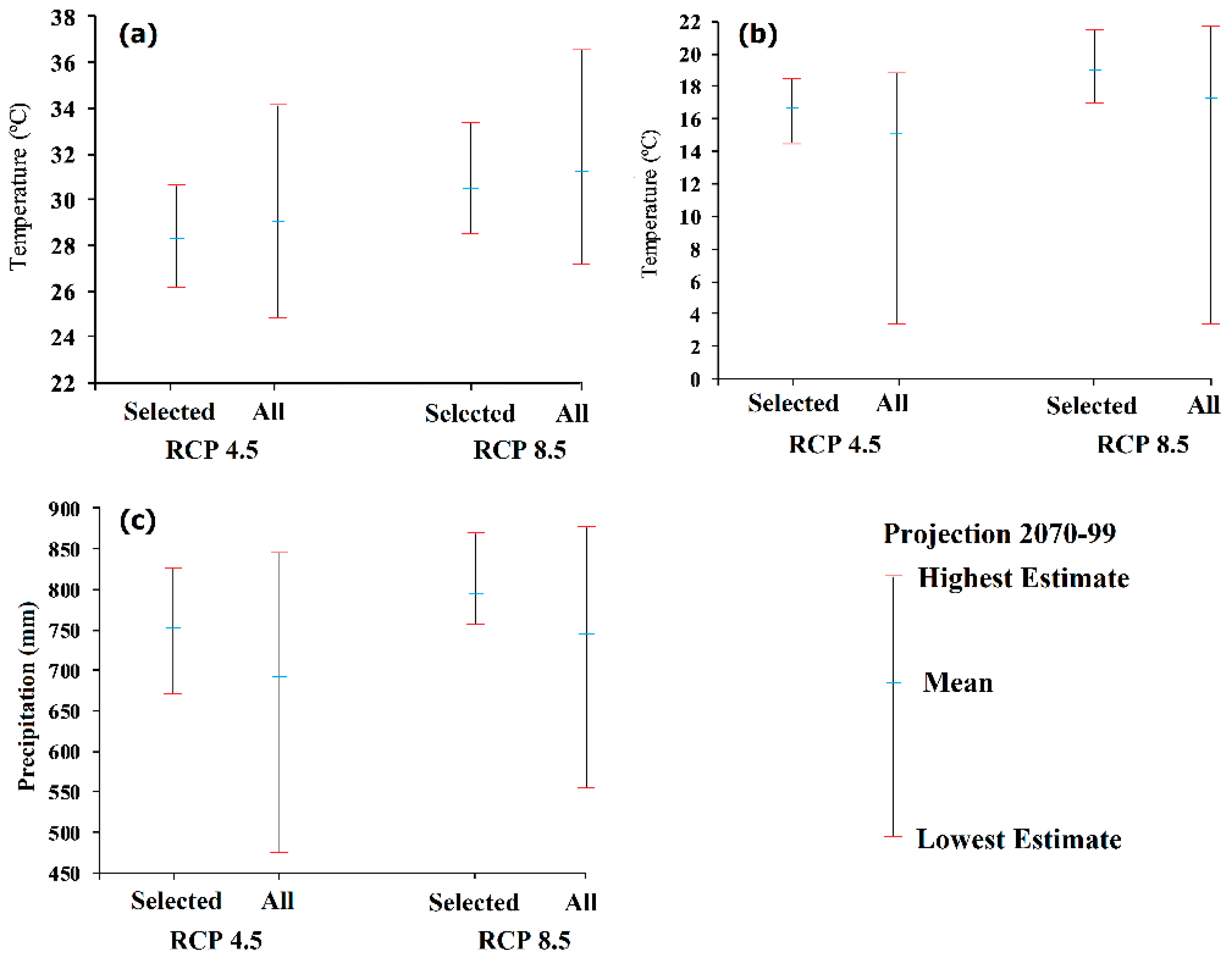
4.5. Future Projections using GCM Ensemble

The selected GCMs are used to project the future changes of temperature and precipitation in Pakistan. The projections obtained from the selected GCMs ensemble are compared with the ensemble of all the 31 GCMs. The projections of the maximum and minimum values of temperature and precipitation during the last part of this century (2070–2099) using the selected GCMs and all 31 GCMs are shown in Figure 7 based on selected RCP scenarios (RCP4.5 and RCP8.5). A significant increase of projection range estimated by all GCMs for all the cases is found in Figure 7. The ensemble mean of the projected temperature changes shifts systematically to the value higher when compared to the full ensemble mean values. Furthermore, the selected best models indicate that the maximum temperatures and precipitation (Figure 7b,c) do not include well-below average outlier models of the full ensemble. On the other hand, a higher increase of both temperature and precipitation is expected under the condition of RCP8.5 compared to RCP4.5.

5. Conclusions

The performance of CMIP5 GCMs in simulating temperature and precipitation is assessed using multiple gridded datasets. In order to understand the influence of gridded data in the selection of GCMs and to identify the common GCMs that perform well for different gridded data and climatic variables. It is known from the results that the performance of GCMs varies according to different gridded data and climatic variables. A trade-off is made for the selection of GCMs based on their performance for different gridded datasets and climatic variables. Six GCMs namely, ACCESS1-3, CESM1-BGC, CMCC-CM, HadGEM2-CC, HadGEM2-ES and MIROC5 are found to be the most suitable for projection of climate of Pakistan according to their performance in reconstructing the historical climate for the period (1961–2005). The selected GCMs are found to be different from those found by [10]. This is due to the selection of GCMs based on different set of gridded data. The results emphasize the use of different gridded data in selection of GCMs to avoid uncertainty of selection. The GCMs are selected in this study solely based on their performances in simulating historical temperature and precipitation. Future projections of GCMs can be considered along with their past performance in the selection of GCMs.

Author Contributions

N.K. and S.S. designed the research and wrote the manuscript. M.S. and K.A. provided technical help with the model design and important analysis. T.I. proposed important additions to the manuscript and N.N. gave critical views on the manuscript for further improvement.

Funding

This research was supported by NRF-2015R1D1A1A02059944 through the National Research Foundation of Korea (NRF), and funded by the Ministry of Education, Science and Technology.

Conflicts of Interest

The authors declare no conflict of interest.

References

  1. Yip, S.; Ferro, C.A.; Stephenson, D.B.; Hawkins, E. A simple, coherent framework for partitioning uncertainty in climate predictions. J. Clim. 2011, 24, 4634–4643. [Google Scholar] [CrossRef]
  2. Maraun, D.; Wetterhall, F.; Ireson, A.; Chandler, R.; Kendon, E.; Widmann, M.; Brienen, S.; Rust, H.; Sauter, T.; Themeßl, M. Precipitation downscaling under climate change: Recent developments to bridge the gap between dynamical models and the end user. Rev. Geophys. 2010, 48. [Google Scholar] [CrossRef] [Green Version]
  3. Lutz, A.F.; ter Maat, H.W.; Biemans, H.; Shrestha, A.B.; Wester, P.; Immerzeel, W.W. Selecting representative climate models for climate change impact studies: An advanced envelope-based selection approach. Int. J. Climatol. 2016, 36, 3988–4005. [Google Scholar] [CrossRef]
  4. Salman, S.A.; Shahid, S.; Ismail, T.; Ahmed, K.; Wang, X.-J. Selection of climate models for projection of spatiotemporal changes in temperature of Iraq with uncertainties. Atmos. Res. 2018, 213, 509–522. [Google Scholar] [CrossRef]
  5. Pour, S.H.; Shahid, S.; Chung, E.-S.; Wang, X.-J. Model output statistics downscaling using support vector machine for the projection of spatial and temporal changes in rainfall of Bangladesh. Atmos. Res. 2018, 213, 149–162. [Google Scholar] [CrossRef]
  6. Mote, P.; Brekke, L.; Duffy, P.B.; Maurer, E. Guidelines for constructing climate scenarios. Eos Trans. Am. Geophys. Union 2011, 92, 257–258. [Google Scholar] [CrossRef]
  7. Srinivasa Raju, K.; Nagesh Kumar, D. Ranking general circulation models for India using TOPSIS. J. Water Clim. Chang. 2015, 6, 288–299. [Google Scholar] [CrossRef]
  8. Warszawski, L.; Frieler, K.; Huber, V.; Piontek, F.; Serdeczny, O.; Schewe, J. The inter-sectoral impact model intercomparison project (ISI–MIP): Project framework. Proc. Natl. Acad. Sci. USA 2014, 111, 3228–3232. [Google Scholar] [CrossRef]
  9. Hidalgo, H.G.; Das, T.; Dettinger, M.; Cayan, D.; Pierce, D.; Barnett, T.; Bala, G.; Mirin, A.; Wood, A.; Bonfils, C. Detection and attribution of streamflow timing changes to climate change in the western United States. J. Clim. 2009, 22, 3838–3855. [Google Scholar] [CrossRef]
  10. Raju, K.S.; Sonali, P.; Kumar, D.N. Ranking of CMIP5-based global climate models for India using compromise programming. Theor. Appl. Climatol. 2017, 128, 563–574. [Google Scholar] [CrossRef]
  11. Ahmed, K.; Shahid, S.; Ali, R.; Harun, S.; Wang, X. Evaluation of the performance of gridded precipitation products over Balochistan Province, Pakistan. Désalin. Water Treat. 2017, 79, 73–86. [Google Scholar] [CrossRef]
  12. Talavera, L. An evaluation of filter and wrapper methods for feature selection in categorical clustering. In Advances in Intelligent Data Analysis VI; Springer: Berlin/Heidelberg, Germany, 2005; pp. 440–451. [Google Scholar]
  13. Maxino, C.; McAvaney, B.; Pitman, A.; Perkins, S. Ranking the AR4 climate models over the Murray-Darling Basin using simulated maximum temperature, minimum temperature and precipitation. Int. J. Climatol. J. R. Meteorol. Soc. 2008, 28, 1097–1112. [Google Scholar] [CrossRef] [Green Version]
  14. Perkins, S.; Pitman, A.; Holbrook, N.; McAneney, J. Evaluation of the AR4 climate models’ simulated daily maximum temperature, minimum temperature, and precipitation over Australia using probability density functions. J. Clim. 2007, 20, 4356–4376. [Google Scholar] [CrossRef]
  15. Knutti, R.; Masson, D.; Gettelman, A. Climate model genealogy: Generation CMIP5 and how we got there. Geophys. Res. Lett. 2013, 40, 1194–1199. [Google Scholar] [CrossRef] [Green Version]
  16. Yokoi, S.; Takayabu, Y.N.; Nishii, K.; Nakamura, H.; Endo, H.; Ichikawa, H.; Inoue, T.; Kimoto, M.; Kosaka, Y.; Miyasaka, T. Application of cluster analysis to climate model performance metrics. J. Appl. Meteorol. Climatol. 2011, 50, 1666–1675. [Google Scholar] [CrossRef]
  17. Jiang, X.; Waliser, D.E.; Xavier, P.K.; Petch, J.; Klingaman, N.P.; Woolnough, S.J.; Guan, B.; Bellon, G.; Crueger, T.; DeMott, C. Vertical structure and physical processes of the Madden–Julian oscillation: Exploring key model physics in climate simulations. J. Geophys. Res. Atmos. 2015, 120, 4718–4748. [Google Scholar] [CrossRef]
  18. Min, S.K.; Hense, A. A Bayesian approach to climate model evaluation and multi-model averaging with an application to global mean surface temperatures from IPCC AR4 coupled climate models. Geophys. Res. Lett. 2006, 33. [Google Scholar] [CrossRef] [Green Version]
  19. Afshar, A.A.; Hasanzadeh, Y.; Besalatpour, A.; Pourreza-Bilondi, M. Climate change forecasting in a mountainous data scarce watershed using CMIP5 models under representative concentration pathways. Theor. Appl. Climatol. 2017, 129, 683–699. [Google Scholar] [CrossRef]
  20. Xuan, W.; Ma, C.; Kang, L.; Gu, H.; Pan, S.; Xu, Y.-P. Evaluating historical simulations of CMIP5 GCMs for key climatic variables in Zhejiang Province, China. Theor. Appl. Climatol. 2017, 128, 207–222. [Google Scholar] [CrossRef]
  21. Taylor, K.E. Summarizing multiple aspects of model performance in a single diagram. J. Geophys. Res. Atmos. 2001, 106, 7183–7192. [Google Scholar] [CrossRef] [Green Version]
  22. Kharin, V.V.; Zwiers, F.W.; Zhang, X. Intercomparison of near-surface temperature and precipitation extremes in AMIP-2 simulations, reanalyses, and observations. J. Clim. 2005, 18, 5201–5223. [Google Scholar] [CrossRef]
  23. Gleckler, P.J.; Taylor, K.E.; Doutriaux, C. Performance metrics for climate models. J. Geophys. Res. Atmos. 2008, 113. [Google Scholar] [CrossRef] [Green Version]
  24. Johnson, F.; Sharma, A. Measurement of GCM skill in predicting variables relevant for hydroclimatological assessments. J. Clim. 2009, 22, 4373–4382. [Google Scholar] [CrossRef]
  25. Fu, G.; Charles, S.P.; Kirshner, S. Daily rainfall projections from general circulation models with a downscaling nonhomogeneous hidden Markov model (NHMM) for south-eastern Australia. Hydrol. Process. 2013, 27, 3663–3673. [Google Scholar] [CrossRef]
  26. Rupp, D.E.; Abatzoglou, J.T.; Hegewisch, K.C.; Mote, P.W. Evaluation of CMIP5 20th century climate simulations for the Pacific Northwest USA. J. Geophys. Res. Atmos. 2013, 118, 10884–10906. [Google Scholar] [CrossRef]
  27. Gu, H.; Yu, Z.; Wang, J.; Wang, G.; Yang, T.; Ju, Q.; Yang, C.; Xu, F.; Fan, C. Assessing CMIP5 general circulation model simulations of precipitation and temperature over China. Int. J. Climatol. 2015, 35, 2431–2440. [Google Scholar] [CrossRef]
  28. Reichler, T.; Kim, J. How well do coupled models simulate today’s climate? Bull. Am. Meteorol. Soc. 2008, 89, 303–312. [Google Scholar] [CrossRef]
  29. Witten, I.H.; Paynter, G.W.; Frank, E.; Gutwin, C.; Nevill-Manning, C.G. KEA: Practical Automated Keyphrase Extraction. In Design and Usability of Digital Libraries: Case Studies in the Asia Pacific; IGI Global: Hershey, PA, USA, 2005; pp. 129–152. [Google Scholar]
  30. Khan, N.; Shahid, S.; Ismail, T.; Ahmed, K.; Nawaz, N. Trends in heat wave related indices in Pakistan. Stoch. Environ. Res. Risk Assess. 2018. [Google Scholar] [CrossRef]
  31. Ahmed, K.; Shahid, S.; Nawaz, N. Impacts of climate variability and change on seasonal drought characteristics of Pakistan. Atmos. Res. 2018, 214, 364–374. [Google Scholar] [CrossRef]
  32. Khan, N.; Shahid, S.; bin Ismail, T.; Wang, X.-J. Spatial distribution of unidirectional trends in temperature and temperature extremes in Pakistan. Theor. Appl. Climatol. 2018, 1–15. [Google Scholar] [CrossRef]
  33. Rohde, R.; Muller, R.; Jacobsen, R.; Muller, E.; Perlmutter, S.; Rosenfeld, A.; Wurtele, J.; Groom, D.; Wickham, C. A new estimate of the average Earth surface land temperature spanning 1753 to 2011. Geoinform. Geostat. Overv. 2013. [Google Scholar] [CrossRef]
  34. Xie, P.; Chen, M.; Shi, W. CPC unified gauge-based analysis of global daily precipitation. In Proceedings of the Preprints, 24th Conference on Hydrology, Atlanta, GA, USA, 17–21 January 2010. [Google Scholar]
  35. Sheffield, J.; Goteti, G.; Wood, E.F. Development of a 50-year high-resolution global dataset of meteorological forcings for land surface modeling. J. Clim. 2006, 19, 3088–3111. [Google Scholar] [CrossRef]
  36. Chaney, N.; Herman, J.; Reed, P.; Wood, E. Flood and drought hydrologic monitoring: The role of model parameter uncertainty. Hydrol. Earth Syst. Sci. 2015, 19, 3239–3251. [Google Scholar] [CrossRef]
  37. Yatagai, A.; Arakawa, O.; Kamiguchi, K.; Kawamoto, H.; Nodzu, M.I.; Hamada, A. A 44-year daily gridded precipitation dataset for Asia based on a dense network of rain gauges. Sola 2009, 5, 137–140. [Google Scholar] [CrossRef]
  38. Yatagai, A.; Kamiguchi, K.; Arakawa, O.; Hamada, A.; Yasutomi, N.; Kitoh, A. APHRODITE: Constructing a long-term daily gridded precipitation dataset for Asia based on a dense network of rain gauges. Bull. Am. Meteorol. Soc. 2012, 93, 1401–1415. [Google Scholar] [CrossRef]
  39. Palazzi, E.; Von Hardenberg, J.; Provenzale, A. Precipitation in the Hindu–Kush Karakoram Himalaya: Observations and future scenarios. J. Geophys. Res. Atmos. 2013, 118, 85–100. [Google Scholar] [CrossRef]
  40. Berkeley Earth Surface Temperature. Available online: http://www.berkeleyearth.org (accessed on 1 June 2018).
  41. Climate Prediction Centre. Available online: http://www.cpc.ncep.noaa.gov/ (accessed on 1 June 2018).
  42. Asian Precipitation—Highly Resolved Observational Data Integration toward Evaluation, (Monsoon Asia). Available online: http://www.chikyu.ac.jp/precip/english/products.html (accessed on 1 June 2018).
  43. Princeton Global Meteorological Forcing Dataset. Available online: http://www.hydrology.princeton.edu (accessed on 1 June 2018).
  44. Intergovernmental Panel on Climate Change. Available online: http://www.ipcc-data.org/sim/gcm_monthly/AR5/Reference-Archive.html (accessed on 1 June 2018).[Green Version]
  45. Wang, L.; Ranasinghe, R.; Maskey, S.; van Gelder, P.M.; Vrijling, J. Comparison of empirical statistical methods for downscaling daily climate projections from CMIP5 GCMs: A case study of the Huai River Basin, China. Int. J. Climatol. 2016, 36, 145–164. [Google Scholar] [CrossRef]
  46. Novaković, J. Toward optimal feature selection using ranking methods and classification algorithms. Yugosl. J. Oper. Res. 2016, 21, 119–135. [Google Scholar] [CrossRef]
  47. Singh, B.; Kushwaha, N.; Vyas, O.P. A feature subset selection technique for high dimensional data using symmetric uncertainty. J. Data Anal. Inf. Process. 2014, 2, 95–105. [Google Scholar] [CrossRef]
  48. Kannan, S.S.; Ramaraj, N. A novel hybrid feature selection via Symmetrical Uncertainty ranking based local memetic search algorithm. Knowl.-Based Syst. 2010, 23, 580–585. [Google Scholar] [CrossRef]
  49. Shreem, S.S.; Abdullah, S.; Nazri, M.Z.A. Hybrid feature selection algorithm using symmetrical uncertainty and a harmony search algorithm. Int. J. Syst. Sci. 2016, 47, 1312–1329. [Google Scholar] [CrossRef]
Figure 1. Topographical map of the study area with the distributed points at 2° × 2°.
Water 10 01793 g001
Figure 2. Spatial distribution of annual average of daily (a) maximum temperature; (b) minimum temperature; and (c) annual total rainfall estimated using different gridded temperature and rainfall data.
Water 10 01793 g002
Figure 3. The concept of mutual information.
Water 10 01793 g003
Figure 4. Ranking of the GCM according to their performance in replicating maximum and minimum temperature and precipitation. The x-axis represents the rank of the GCM while the y-axis represents the GCM number as described in Table 2. The color bar shows the number of grid points.
Water 10 01793 g004
Figure 5. The geographical distribution of best performing GCMs in simulating: (a) maximum temperature; (b) minimum temperature; and (c) precipitation over Pakistan for different gridded datasets. The number in the figure represent the GCM as mentioned in Table 2.
Water 10 01793 g005
Figure 6. Score estimated for different GCMs in simulating the maximum temperature (upper panel), the minimum temperature (middle panel) and the precipitation (lower panel) for Pakistan.
Water 10 01793 g006
Figure 7. The projections of (a) maximum temperature; (b) minimum temperature; and (c) precipitation during 2070–2099 obtained using the selected GCMs and all GCMs.
Water 10 01793 g007
Table 1. The description of the gridded datasets used in the study.
ProductsSourcePeriodSpatial ResolutionClimate Variable
BEST [33]Berkley Earth Surface Temperature [40](1960–2013)1° × 1°Daily Temp.
CPC [34]Climate Prediction Centre [41](1979–present)0.5° × 0.5°Daily Temp. and Precipitation
APHRODITE [37]Asian Precipitation—Highly Resolved Observational Data Integration Toward Evaluation, (Monsoon Asia) [42](1951–2007)0.5° × 0.5°Daily Precipitation
PGF [35]Princeton Global Meteorological Forcing [43](1948–2010)0.25° × 0.25°Daily Temp. and Precipitation
Table 2. The Coupled Model Intercomparison Project Phase 5 (CMIP5) general circulation models (GCMs) used in this study for the selection of an ensemble for Pakistan.
GCM No.GCM NameDeveloperResolution
1ACCESS1-0Commonwealth Scientific and Industrial Research Organisation–Bureau of Meteorology, Australia1.9 × 1.2
2ACCESS1-3
3bcc-csm1-1-mBeijing Climate Centre, China2.8 × 2.8
4bcc-csm1-11.1 × 1.1
5BNU-ESMBeijing Normal University, China2.8 × 2.8
6CanESM2Canadian Centre for Climate Modelling and Analysis, Canada2.8 × 2.8
7CCSM4National Centre for Atmospheric Research
USA
0.94 × 1.25
8CESM1(BGC)0.94 × 1.25
9CMCC-CMCentro Euro-Mediterraneo sui Cambiamenti Climatici, Italy0.7 × 0.7
10CMCC-CMS1.9 × 1.9
11CNRM-CM5Centre National de Recherches Météorologiques, Centre, France1.4 × 1.4
12CSIRO-Mk3-6-0Commonwealth Scientific and Industrial Research Organization, Australia1.9 × 1.9
13EC-EARTHEC-EARTH consortium published at the Irish Centre for High-End Computing, Netherlands/Ireland1.1 × 1.1
14FGOALS-g2Institute of Atmospheric Physics, Chinese Academy of Sciences, China2.8 × 2.8
15GFDL-CM3Geophysical Fluid Dynamics Laboratory, USA2.5 × 2.0
16GFDL-ESM2G2.5 × 2.0
17GFDL-ESM2M2.5 × 2.0
18GISS-E2-RNASA/GISS (Goddard Institute for Space Studies), USA2.5 × 2.0
19HadGEM2-CCMet Office Hadley Centre, UK1.9 × 1.2
20HadGEM2-ES1.9 × 1.2
21INMCM4.0Institute of Numerical Mathematics, Russia2.0 × 1.5
22IPSL-CM5A-LRInstitut Pierre Simon Laplace, France3.7 × 1.9
23IPSL-CM5A-MR2.5 × 1.3
24IPSL-CM5B-LR3.7 × 1.9
25MIROC-ESM-CHEMThe University of Tokyo, National Institute for Environmental Studies, and Japan Agency for Marine-Earth Science and Technology, Japan2.8 × 2.8
26MIROC-ESM2.8 × 2.8
27MIROC51.4 × 1.4
28MPI-ESM-LRMax Planck Institute for Meteorology, Germany1.9 × 1.9
29MPI-ESM-MR1.9 × 1.9
30MRI-CGCM3Meteorological Research Institute, Japan1.1 × 1.1
31NorESM1-MMeteorological Institute, Norway2.5 × 1.9
Table 3. The scores obtained from different GCMs according to their performance estimated using symmetric uncertainty and conventional statistics.
GCM No.Model NameScore (SU)Rank (SU)Score (R2)Score (NRMSE)Average (R2 + NRMSE)Rank (R2 + NRMSE)
1ACCESS1-01.66153.013.773.3915
2ACCESS1-36.7733.075.984.026
3bcc-csm1-10.00183.301.902.6021
4bcc-csm1-1-m0.00182.843.533.1918
5BNU-ESM2.69103.063.533.2916
6CanESM22.21123.983.043.5112
7CCSM41.70144.502.493.4913
8CESM1-BGC3.4875.481.583.5311
9CMCC-CM5.6452.844.923.888
10CMCC-CMS0.00185.072.403.739
11CNRM-CM50.00183.161.512.3324
12CSIRO-Mk3-6-014.2513.885.694.793
13EC-EARTH0.00181.942.222.0828
14FGOALS-g20.00183.293.103.2017
15GFDL-CM33.4384.012.773.3914
16GFDL-ESM2G0.00181.491.061.2830
17GFDL-ESM2M0.00181.832.992.4123
18GISS-E2-R0.00184.933.474.204
19HadGEM2-CC1.83134.242.873.5610
20HadGEM2-ES2.9992.523.382.9520
21INMCM40.00181.763.262.5122
22IPSL-CM5A-LR0.00181.922.592.2625
23IPSL-CM5A-MR3.9362.985.134.055
24IPSL-CM5B-LR0.00181.083.382.2326
25MIROC51.41173.502.422.9619
26MIROC-ESM0.00180.762.111.4429
27MIROC-ESM-CHEM1.41160.923.472.1927
28MPI-ESM-LR11.3724.695.335.011
29MPI-ESM-MR0.00180.001.680.8431
30MRI-CGCM32.66113.174.753.967
31NorESM1-M6.3045.104.504.802
Table 4. The scores obtained by different GCMs according to their performance based on different gridded dataset.
ModelMax TemperatureMin TemperaturePrecipitation
BESTCPCPGFScoreBESTCPCPGFScoreAPHCPCPGFScore
ACCESS1-01.33.00.71.70.02.50.20.91.32.73.52.5
ACCESS1-36.07.07.36.88.79.011.29.71.54.03.93.1
bcc-csm1-1-m1.21.81.21.40.00.00.00.00.51.91.11.2
bcc-csm1-11.50.50.30.70.20.00.20.11.71.12.21.6
BNU-ESM2.14.02.02.72.00.20.30.92.00.02.21.4
CanESM20.73.82.22.22.53.13.63.10.50.20.30.3
CCSM41.11.82.21.73.02.92.62.80.21.02.31.2
CESM1-BGC4.33.82.33.53.94.44.14.12.25.45.14.2
CMCC-CM7.74.54.85.67.43.19.06.52.02.32.72.3
CMCC-CMS2.40.70.71.33.22.43.43.00.72.60.51.2
CNRM-CM50.30.00.00.10.90.50.60.71.55.94.54.0
CSIRO-Mk3-6-011.614.017.214.311.18.012.910.70.00.00.00.0
EC-EARTH0.20.00.00.12.01.01.91.63.816.313.811.3
FGOALS-g20.00.20.50.23.03.42.22.90.00.71.00.6
GFDL-CM33.75.51.13.40.82.71.91.80.01.01.40.8
GFDL-ESM2G0.01.50.00.50.20.50.50.40.00.50.00.2
GFDL-ESM2M0.50.20.80.50.00.30.00.11.00.00.00.3
GISS-E2-R0.30.20.00.20.00.20.00.10.90.82.51.4
HadGEM2-CC3.51.20.81.83.74.02.33.32.28.96.35.8
HadGEM2-ES5.01.12.93.02.65.24.94.31.35.84.43.8
INMCM40.81.30.50.90.00.00.00.01.30.51.51.1
IPSL-CM5A-LR0.30.40.00.20.01.30.30.50.00.00.30.1
IPSL-CM5A-MR5.51.74.53.90.00.00.00.00.50.00.00.2
IPSL-CM5B-LR0.70.01.20.60.01.01.00.70.30.20.90.5
MIROC-ESM-CHEM0.20.20.30.21.70.20.50.81.23.82.42.4
MIROC-ESM0.00.00.00.00.51.80.50.93.04.52.53.3
MIROC51.11.02.11.41.83.50.01.812.59.014.211.9
MPI-ESM-LR11.012.710.411.48.76.24.46.40.30.20.20.2
MPI-ESM-MR0.00.81.40.70.84.72.02.51.00.30.00.4
MRI-CGCM31.01.75.22.75.44.05.44.90.00.00.30.1
NorESM1-M6.15.47.56.35.84.04.04.60.00.50.30.3
Table 5. The GCMs received the highest scores in replicating temperature and precipitation at all the grid points over Pakistan. The selected GCMs are shown in bold fonts.
GCMMax TemperatureMin TemperaturePrecipitation
ACCESS1-01.70.02.5
ACCESS1-36.89.73.1
bcc-csm1-10.00.01.6
bcc-csm1-1-m0.00.01.2
BNU-ESM2.70.01.4
CanESM22.23.10.0
CCSM41.72.80.0
CESM1-BGC3.54.14.2
CMCC-CM5.66.52.3
CMCC-CMS0.03.01.2
CNRM-CM50.00.04.0
CSIRO-Mk3-6-014.310.70.0
EC-EARTH0.00.011.3
FGOALS-g20.02.90.0
GFDL-CM33.41.80.0
GFDL-ESM2G0.00.00.0
GFDL-ESM2M0.00.00.0
GISS-E2-R0.00.01.4
HadGEM2-CC1.83.35.8
HadGEM2-ES3.04.33.8
INMCM40.00.00.0
IPSL-CM5A-LR0.00.00.0
IPSL-CM5A-MR3.90.00.0
IPSL-CM5B-LR0.00.00.0
MIROC51.41.811.9
MIROC-ESM0.00.03.3
MIROC-ESM-CHEM0.00.02.4
MPI-ESM-LR11.46.40.0
MPI-ESM-MR0.02.50.0
MRI-CGCM32.74.90.0
NorESM1-M6.34.60.0

