Using SCADA to Detect and Locate Bursts in a Long-Distance Water Pipeline

Abstract

Pipe bursting is a serious problem for water supply systems. We propose a two-step burst detection and localization method for a long-distance water transportation pipeline. First, we use the Dempster–Shafer theory, an effective inference method for processing uncertain information, and combine two risk functions to identify a pipe burst. Then we identify the location of the burst point using a hydraulic model. The method is prototyped on a transportation pipeline in Guangzhou, China and tested with one-year historical records. The detection system correctly identified all the bursts and the alarm rate is acceptable for the system inspectors (average: two alarms/month). The burst location is identified within the acceptable limits of accuracy.

1. Introduction

Pipe leaks and bursts are common in water supply systems for reasons such as poor construction quality, improper operation management, and abrupt temperature changes. Burst/leakage results in wasted water, financial loss, water pollution, and serious social consequences. Long-distance water transportation pipelines (pipes connecting the water source to the water treatment plant) use pipes larger in diameter than urban water distribution systems and have a higher working pressure and greater flow velocity. It is critical to monitor the water transportation system for leakage because a burst can affect downstream water supply components, thus causing serious damage to the whole water supply system, such as the interruption of water supply, real estate damage, and water/energy waste. If a leak can be identified promptly, losses will be greatly reduced.

Water companies are concerned about leakage and burst pipes, which are the subject of considerable research in the field of water distribution systems. Li et al. [1] classified leakage detection methods and techniques into two categories: hardware-based methods and software-based methods. The hardware-based methods utilize hardware equipment for leak detection with a relatively high accuracy (e.g., vibro-acoustic techniques, listening sticks/correlators, gas injection techniques, thermography, ground penetrating radar, etc.). Leak detection techniques based on vibro-acoustic measurements are widely adopted by monitoring the vibroacoustic phenomena of active leaks [2]. It includes vibration monitoring and Acoustic–Emission-based techniques. The vibration-based method is proposed to detect and quantify leaks through analyzing vibrational response of the pipeline [3,4,5]. The Acoustic–Emission-based techniques is a non-intrusive evaluation method that can be applied for leak detection by monitoring the AE signals produced from leaks [6].

The other category consists of software-based methods that use real-time monitoring data, and include hydraulic model-based methods, transient-based methods, and dedicated data mining methods. Baghdadi and Mansy [7] created a mathematical model to locate a pipe leak by analyzing the change in pressure before and after the leak. Methods using hydraulic information (generally flow and pressure data) obtained by supervisory control and data acquisition (SCADA) have been widely studied. Pudar and Liggett [8] proposed a leakage detection method based on the inverse analysis of pressure and flow data. Misiunas et al. [9] used pressure wave data to find the location of a burst by measuring the arrival time of a transient wave and inferring the size of the burst from the wave magnitude. Lee et al. [10] analyzed the resonance peak patterns of the system frequency response diagram (FRD) to detect leaks. Bicik et al. [11] developed a methodology that used the Dempster‒Shafer (D–S) theory with the outputs of several models to increase the accuracy of leak localization. Srirangarajan et al. [12] used multiscale wavelet analysis of high-frequency data to detect and locate pipe burst events.

Recently, data mining methods have been regarded as promising tools for burst detection. Mounce and Machell [13] used both static and time-delayed artificial neural networks (ANNs) on different classifications of time series to detect leakage and bursts. Further development and field validation are described in their subsequent articles [14,15]. Ye and Fenner [16] developed a Kalman filtering method to detect pipe leakage by measuring flow and pressure at district metering locations. Based on this, Choi et al. [17] analyzed the effect of the sampling interval on Ye’s Kalman filter model and proposed a new sampling algorithm to improve bursts prediction ability. Ye and Fenner [18] used weighted least squares to derive a polynomial function to fit the historical flow data for automatic leakage detection. Lin et al. [19] developed a hybrid heuristic approach based on the ordinal optimization algorithm and symbiotic organism search to identify leaks. It was found that this method has the ability to determine leak numbers, locations, and size. Wu et al. [20] used a clustering algorithm to detect pipe leakage in a real DMA, and this algorithm exhibited good performance with a relatively low false positive rate. Wu and Liu [21] examined the applicability and limitations of existing data-driven approaches, and recommended comprehensive performance evaluation in future work. However, methods using pressure wave data need high-frequency sensors, which are rarely used in water distribution systems because of high costs and instability. Data mining approaches show a high false alarm rate due to inaccurate monitored data, which makes their current use for water distribution systems impractical and unrealistic.

Most of the current research focuses on identifying bursts/leakage in water distribution networks; little is devoted to the detection and localization of bursts in long-distance water transportation pipelines. This paper describes a convenient and practical method for detecting and locating long-distance pipeline leaks in two stages. First, we explain how the D–S theory can be used to detect a pipe burst. The abnormal risk values of pressure and flow to be used are derived from monitored data. Second, we show how the localization equation is used to locate the burst point using pressure fluctuation between the upstream and downstream monitors. We use a case study to show how this approach is applied to a long-distance pipe monitoring system. The feasibility and applicability of the method are summarized and discussed. Finally, we make some pertinent suggestions for further research.

2. Pipe Burst Detection

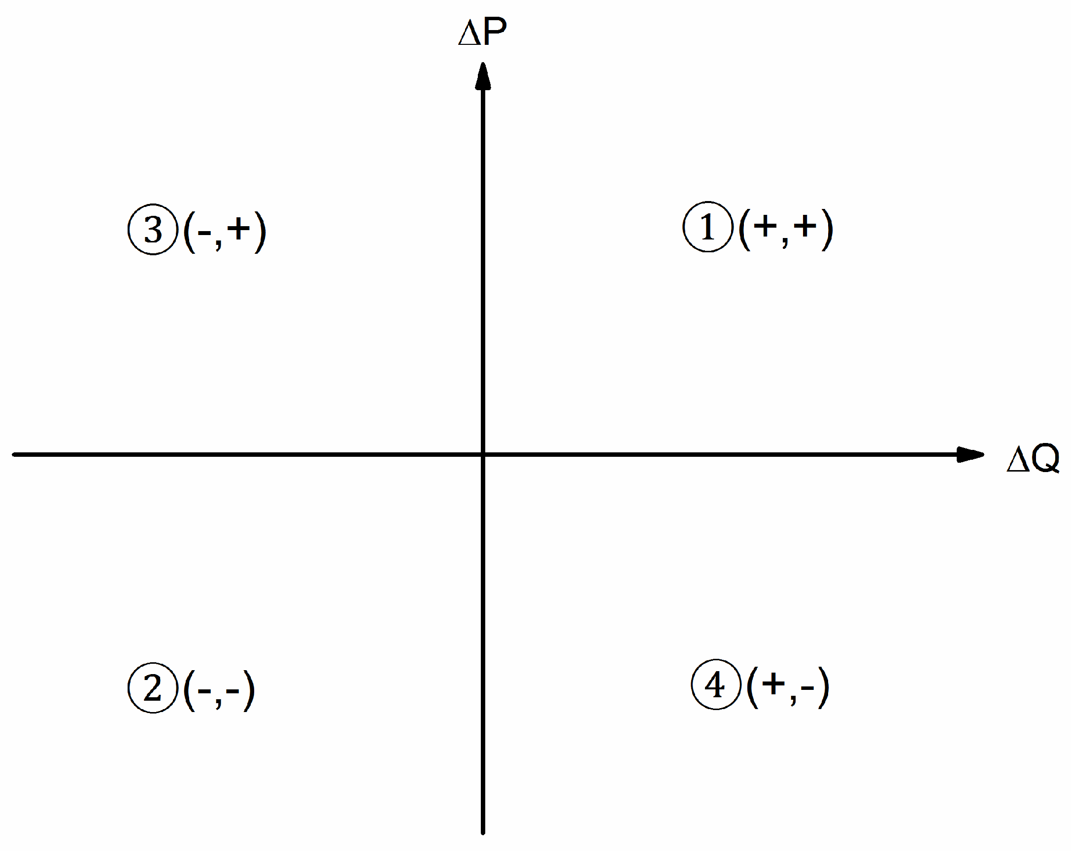
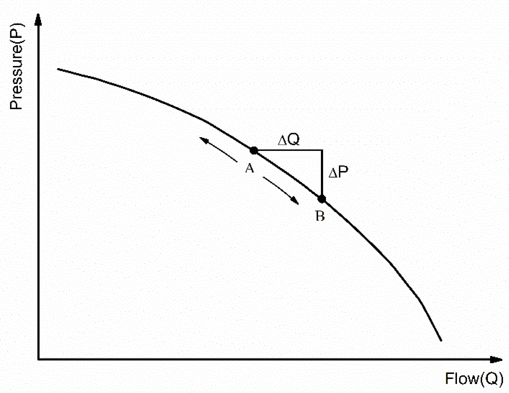
2.1. State Changes of Pressure and Flow at Pumping Station

Major water transportation pipelines are especially important for the safety of a city water supply. Many sensors are installed along the pipelines to monitor their status, as shown in Figure 1. Usually, a flow sensor and a pressure sensor are fitted at the pump station to record the flow rate and the pressure at the pipeline inlet. Other sensors are installed every few kilometers.

Changes in pressure and flow in the water pipe are related to the operation of pumps and variability in demand. There are four states of change in pressure and flow, which are shown in Figure 2:

State 1

When the number of operating pumps increases, the pressure and flow both increase (ΔP and ΔQ are positive);

State 2

When some pumps are shut off, the pressure drops and the flow also decreases (ΔP and ΔQ are negative);

State 3

If the flow decreases, the pressure rises when the number of pumps operating remains constant (ΔQ is negative and ΔP is positive); and

State 4

If the flow increases, the pressure descends when the number of pumps stays constant (ΔQ is positive and ΔP is negative).

In most cases, the number of pumps running is constant. When the flow increases, the pump state will change from A to B (Figure 3), where the pressure decreases by ΔP and the flow increases by ΔQ. If the absolute values of ΔP and ΔQ are too large, a burst may have occurred. Therefore, ΔP and ΔQ are, in effect, information to identify a pipe burst. The threshold values of ΔP and ΔQ can be determined from their statistical characteristics.

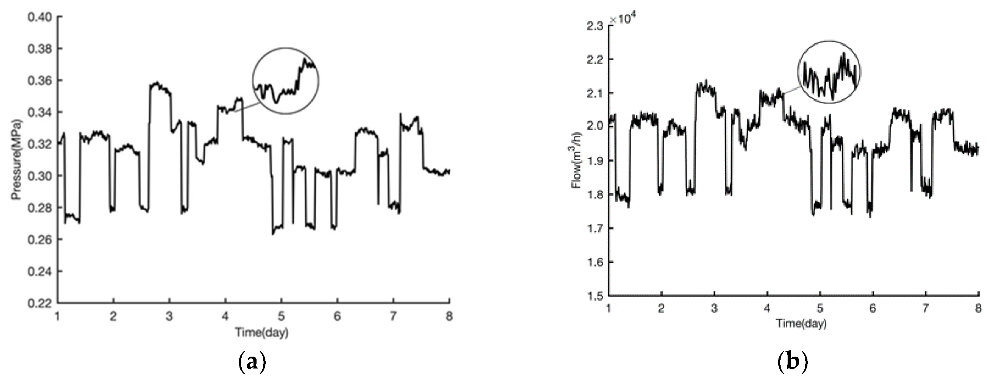
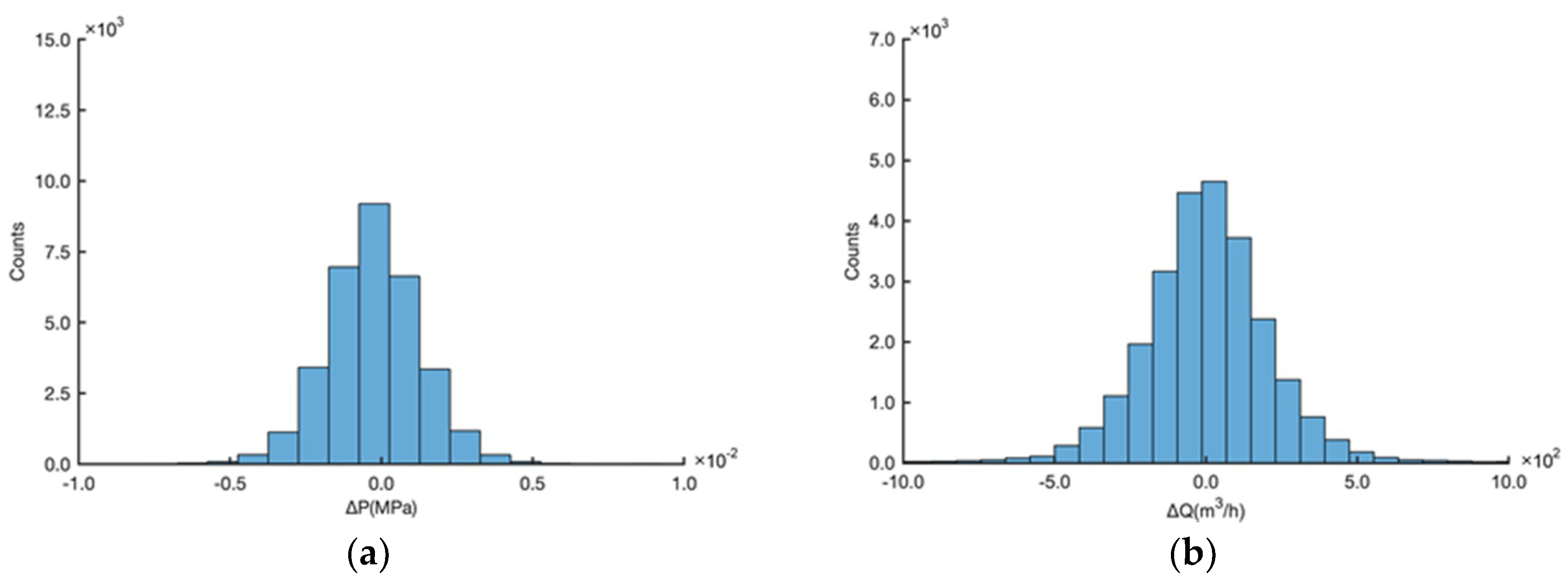
2.2. Pressure and Flow Fluctuation Distributions

Pressure and flow are not constant because they vary with demand. In this section, historical data for a transportation pipeline in Guangzhou are used to find a statistical pattern. Pressure and flow at the pump station are shown in Figure 4. On a macro scale, pressure and flow increase or decrease simultaneously, which is represented by states 1 and 2 in Figure 2. The monitoring data varies in a wide range and are different every day, which can be explained by the operation of pumps according to the demand variation of downstream. At a micro level, they change within a certain range because of water plant regulation, and the tiny random fluctuations can be seen in the enlarged view.

The three-sigma (3σ) rule-of-thumb is widely used in experimental random variable processing. However, more evidence is required to convince engineers to use the rule in practical applications. Pressure and flow are not normally distributed, but their variations (ΔP and ΔQ) approach normal distributions. Zhao and Cheng [22] found that in a water distribution system, the cumulative probability curves of pressure and flow fluctuation fit the normal distribution within the probability range 5–95%, but they are significantly different outside this range. The inflection point is located within 2–3 times standard deviation. Similarly, in a long-distance pipeline, the histogram of ΔP or ΔQ at the pump station is approximately a normal distribution, as shown in Figure 5. Figure 6 shows the cumulative probability of ΔP and ΔQ. The straight line is the normal distribution function (an error function) on a stretched coordinate. The vertical axes show the cumulative probability of ΔP or ΔQ. The 3σ rule indicates that data within the probability range 3–97% are normal, while data outside this range have a high probability of being abnormal.

2.3. Abnormality Risk Function

Traditional methods use a threshold value of pressure or flow to determine whether there is a burst. However, fluctuating data can occasionally surpass the threshold but may not necessarily indicate a burst. Using an indicator such as burst probability is more suitable for this kind of uncertain event. In this section, we describe how a risk function based on observed data is used to evaluate the abnormality of pressure and flow. Since fluctuations of pressure and flow are approximately normally distributed, we use the Gaussian error function as the risk function. As discussed above, decreasing pressure with increasing flow may indicate a burst event, and the risk functions for pressure and flow fluctuation can be expressed as in Equations (1) and (2):

$$\mathrm{F}(\Delta {\mathrm{P})}_{\mathrm{abnormal}}={\displaystyle {\int }_{\Delta \mathrm{P}}^{+\infty }\frac{1}{\sqrt{2\pi }\cdot {\mathsf{\sigma }}_{\Delta \mathrm{P}}}}{e}^{-{(x-{\mathsf{\mu }}_{\Delta \mathrm{P}})}^2/(2{\mathsf{\sigma }}_{\Delta \mathrm{P}}{}^2)}d(x)$$

(1)

$$\mathrm{F}(\Delta {\mathrm{Q})}_{\mathrm{abnormal}}={\displaystyle {\int }_{-\infty }^{\Delta \mathrm{Q}}\frac{1}{\sqrt{2\pi }\cdot {\mathsf{\sigma }}_{\Delta \mathrm{Q}}}}{e}^{-{(x-{\mathsf{\mu }}_{\Delta \mathrm{Q}})}^2/(2{\mathsf{\sigma }}_{\Delta \mathrm{Q}}{}^2)}d(x),$$

(2)

where µ_ΔP is the mean of pressure fluctuations; σ_ΔP is the mean square deviation of pressure fluctuations; µ_ΔQ is the mean of flow fluctuations; and σ_ΔQ is the mean square deviation of flow fluctuations.

2.4. Combining Pressure and Flow Risk Functions

It is likely there is a burst only when both the pressure drops and the flow increases beyond a certain range. Thus, combining the two risk functions can provide more reliable burst detection, considering the uncertainty, inaccuracy, and incompleteness of the data. D–S theory, or evidence theory, is widely used in fuzzy reasoning and expert systems. It was first developed by Dempster and subsequently improved by Shafer [23], and it effectively represents uncertainty.

In D–S theory, a set Θ that consists of incompatible (i.e., mutually exclusive) basic propositions is called the frame of discernment, and the set consisting of all possible combinations of the propositions of Θ is the power set 2^Θ. If B is a nonempty subset of Θ, its probability assignment function is denoted by m(B), which represents trust in the degree of evidential support for proposition B:

$$m(B):2^{\Theta }\to [0,1]$$

(3)

$${\displaystyle {\sum }_{B\subseteq \Theta }m(B)}=1.$$

(4)

If m(B) > 0, B is called the focal element. For the empty set Φ, m(Φ) = 0.

On the basis of the probability assignment function, the belief function Bel is defined as:

$$Bel(A):2^{\Theta }\to [0,1]$$

(5)

$$Bel(A)={\displaystyle \sum }_{B_i\subseteq A}m(B_i),$$

(6)

where A is a non-empty subset of Θ, Bel(A) is the belief function of A, which is the sum of the basic beliefs of all its subsets B_i (Equation (6)). Bel(Φ) is also zero. Another fundamental function of D–S theory, the plausibility function Pl, is defined as:

$$Pl(A):2^{\Theta }\to [0,1]$$

(7)

$$Pl\left(A\right)=1-Bel(\overline{A}),$$

(8)

where A is a non-empty subset of Θ, and Bel($\overline{A}$) is the degree of trust in the inverse (negation) of proposition A. In other words, Pl(A) gives an upper limit for judging the truth of A.

If two basic probability assignment functions m₁ and m₂ are given and their corresponding focal elements are A_i and B_j, the combination rule of D–S is defined by:

$$m(A)=\{\begin{array}{c}\frac{{\displaystyle \sum _{Ai\cap Bj=A}m1(Ai)m2(Bj)}}{1-K},A\ne \varphi \\ 0,A=\varphi \end{array},$$

(9)

$$K={\displaystyle \sum _{Ai\cap Bj=\varphi }m1(Ai)m2(Bj)}$$

(10)

where K is a coefficient that reflects the degree of conflict among various evidences, and 1/(1 − K) is the normalization factor. If K < 1, the combined function m(A) exists; otherwise, m(A) does not exist, which means that m₁ and m₂ contradict each other.

Combining the pressure and flow risk functions of Equations (1) and (2), a burst detection method can be formulated using Equation (9). More details and examples will be introduced in Section 4.

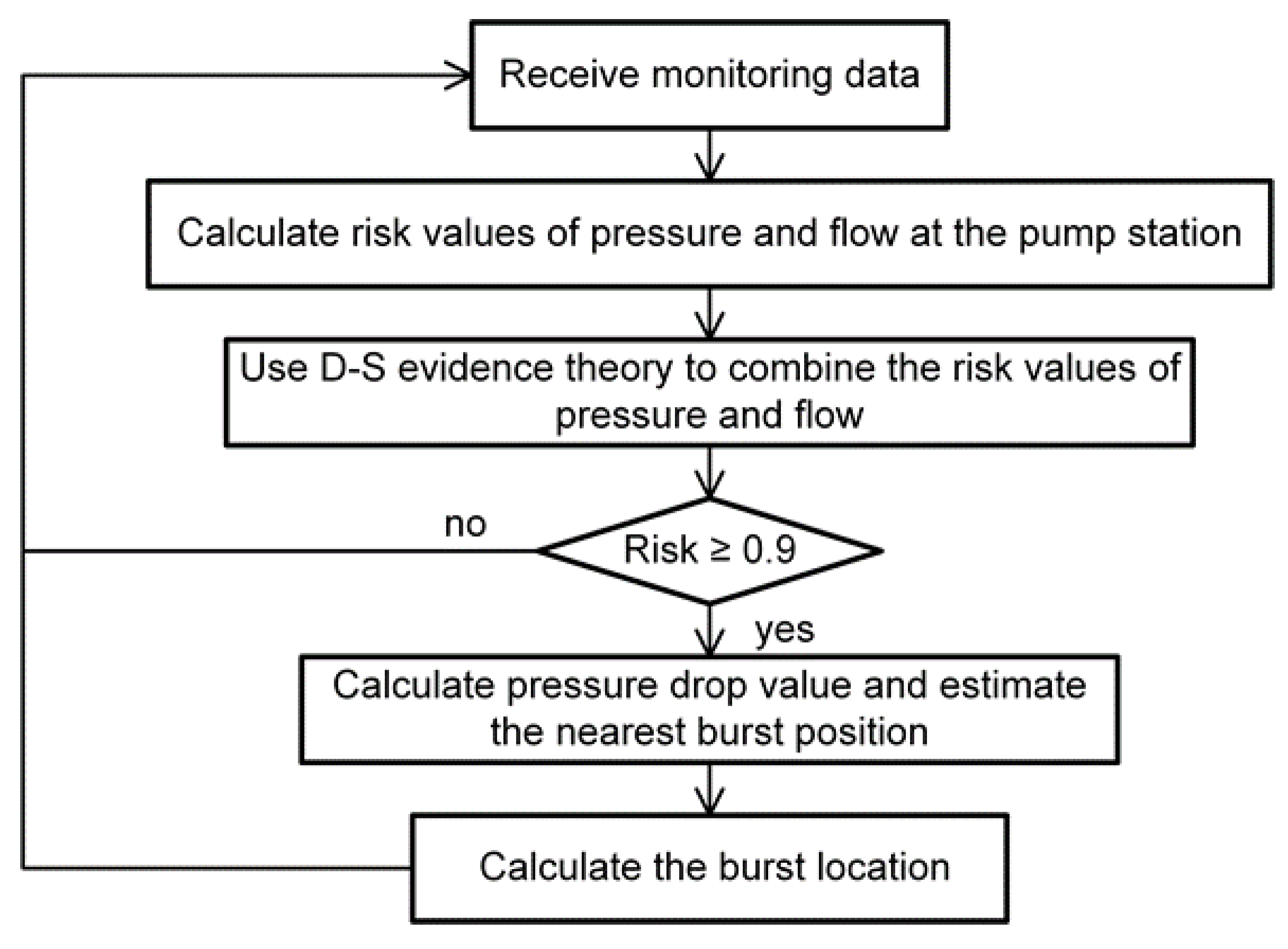
3. Pipe Burst Localization

The previous section described the burst detection method. When a pipe burst is observed, the objective is to locate the burst point as soon as possible. The frictional head loss is calculated as:

$${\delta }_f=SL{\mathrm{Q}}^n,$$

(11)

where S is the specific resistance of the pipeline; n is an exponent (the Reynolds number of a large-diameter pipe is usually >10⁶, which means the drag of the pipe is proportional to speed squared, so usually n = 2); L is the length of the pipe section; and Q is the flow.

Assuming that the elevation of the pipe is constant, both water head and pressure fall along the pipe (Figure 7). In normal conditions, the pressure drop curve is a straight line (line A). After a leak or burst occurs, the pressure at the pump station drops by ΔP₁, and the slope of the water head line will change at the burst point. The slope of the line B₁ increases as the upstream flow increases. The pressure difference ΔP₂ also increases between B₁ and C (C is parallel to line A) in the outlet direction of the pipe, due to the burst flow. In contrast, the slope of the line B₂ decreases and the corresponding ΔP₂ decreases too.

Pipe monitoring scheme is shown in Figure 8. The pressure difference between the two pressure sensors is calculated as:

$$({\mathrm{P}}_1+\rho gz1+\frac{\rho v^2}{2})-({\mathrm{P}}_2+\rho gz2+\frac{\rho v^2}{2})=SL{\mathrm{Q}}_0^2$$

(12)

$${\mathrm{P}}_1-{\mathrm{P}}_2=SL{\mathrm{Q}}_0^2+C,$$

(13)

where P₁ and P₂ are the upstream and downstream pressures under regular operating conditions; C = $\rho g(z2-z1)$; and Q₀ is the normal flow. After a burst occurs at location x, Equation (13) becomes:

$$\{\begin{array}{l}{\mathrm{P}}_1^{\prime }-{\mathrm{P}}_2^{\prime }=Sx{\mathrm{Q}}_1^2+S(L-x){\mathrm{Q}}_2^2+C\\ {\mathrm{Q}}_1={\mathrm{Q}}_2+\Delta \mathrm{Q}\end{array},$$

(14)

where x is the distance between the burst point and the upstream pressure sensor; P’₁ and P’₂ are the upstream and downstream pressures after the burst; Q₁ and Q₂ are the upstream and downstream flows; and ΔQ is the burst flow. The burst location is calculated by:

$$x=\frac{{\mathrm{P}}_1^{\prime }-{\mathrm{P}}_2^{\prime }-({\mathrm{P}}_1-{\mathrm{P}}_2)}{S[{\left({\mathrm{Q}}_2+\Delta \mathrm{Q}\right)}^2-{\mathrm{Q}}_2{}^2]}.$$

(15)

To minimize the measurement errors, the average data of several monitoring points are used to estimate the burst position. For example, as there are four pressure sensors around the pipe bust point (Figure 8), a burst point is estimated from selected pairs of sensors:

Estimated burst position from sensors a and c:

$$x_{ac}=\frac{{\mathrm{P}}_a^{\prime }-{\mathrm{P}}_c^{\prime }-({\mathrm{P}}_a-{\mathrm{P}}_c)}{S_{ac}[{(\mathrm{Q}+\Delta \mathrm{Q})}^2-{\mathrm{Q}}^2]}.$$

Estimated burst position from sensors a and d:

$$x_{ad}=\frac{{\mathrm{P}}_a^{\prime }-{\mathrm{P}}_d^{\prime }-({\mathrm{P}}_a-{\mathrm{P}}_d)}{S_{ad}[{(\mathrm{Q}+\Delta \mathrm{Q})}^2-{\mathrm{Q}}^2]}.$$

Estimated burst position from sensors b and c:

$$x_{bc}=\frac{{\mathrm{P}}_b^{\prime }-{\mathrm{P}}_c^{\prime }-({\mathrm{P}}_b-{\mathrm{P}}_c)}{S_{bc}[{(\mathrm{Q}+\Delta \mathrm{Q})}^2-{\mathrm{Q}}^2]}.$$

Estimated burst position from sensors b and d:

$$x_{bd}=\frac{{\mathrm{P}}_b^{\prime }-{\mathrm{P}}_d^{\prime }-({\mathrm{P}}_b-{\mathrm{P}}_d)}{S_{bd}[{(\mathrm{Q}+\Delta \mathrm{Q})}^2-{\mathrm{Q}}^2]}.$$

The final estimated average value is:

$$\overline{x}=\frac{{\displaystyle \sum }{x}_n}{n}=\frac{2l_a+2l_b+x_{ac}+x_{ad}+x_{bc}+x_{bd}}{4},$$

where x_ac and x_ad are the distances between the burst point and sensor a; x_bc and x_bd are the distances between the burst point and the sensor b; l_a and l_b are the distances from the pump station to the sensors a and b; $\overline{x}$ is the estimated average distance from the pump station; Q is the flow before the burst event; and Q + ΔQ is the flow after the burst event. The flow data are measured from the pump station, and pressure data are gathered from each monitoring point every 5 min.

The resistance parameter S in Equation (15) needs to be fitted according to the historical data. Specific results will be introduced in the next section.

4. Case Study

A monitoring system based on the burst/leakage detection and location method described above was successfully implemented at a water treatment plant in China. Two parallel pipelines (diameter 2.200 m) connect the reservoir to the water treatment plant. The length of a single pipeline is 22.770 km, and the average flow in each pipeline is about 19,800 m³/h. The dual pipeline is constructed mostly of steel pipes, and some pipe sections have been replaced by GRP sand pipes or ductile iron pipes during maintenance. Sixteen remote-transmitting pressure sensors and two flow sensors are installed along each pipeline. The pipeline configuration is shown in Figure 9.

The pipe burst/leakage detection system is installed on a computer server. It continuously monitors the two pipes and generates evaluation results every 5 min. When the value of the combined risk functions surpasses any of the three different risk thresholds (which will be discussed in the next section), the system will show a red, orange, or yellow alarm. Figure 10 shows the monitoring station web page. The underlying flowchart for this system is shown in Figure 11.

4.1. Pipe Burst Detection

4.1.1. Risk Threshold

The risk threshold is a significant parameter for the real-time monitoring system. If the threshold level is too low, too many alarms will habituate the inspectors, who will gradually learn to ignore the alarms. If the threshold level is too high, genuine leakages may be missed or incorrectly trigger the alarm. A reasonable threshold level is critical to maintain a balance between safety (i.e., accurate detection and appropriate alarm) and sensitivity. We calculate risk values for 2014 and set three alarm levels (red, orange, and yellow) considering the principles above, as shown in

Table 1. Counts and proportion of data in different risk intervals.

Pressure Risk			Flow Risk			Combined Risk
Risk	Counts	Proportion	Risk	Counts	Proportion	Risk	Counts	Proportion
0.0–0.1	813	2.32%	0.0–0.1	615	1.75%	0.0–0.1	7901	22.55%
0.1–0.2	123	0.35%	0.1–0.2	1677	4.78%	0.1–0.2	26,525	75.70%
0.2–0.3	31,608	90.21%	0.2–0.3	24,359	69.51%	0.2–0.3	403	1.15%
0.3–0.6	1807	5.15%	0.3–0.6	7848	22.39%	0.3–0.6	116	0.33%
0.6–0.9	380	1.08%	0.6–0.9	362	1.03%	0.6–0.9	71	0.20%
0.9–1.0	309	0.88%	0.9–1.0	179	0.51%	0.9–1.0	24	0.07%

. The highest risk level is red when the data meet the following conditions: combined risk ≥0.9; flow risk ≥0.8; and pressure risk ≥0.8. The orange and yellow risk criteria are 0.6–0.9 and 0.3–0.6. The 2014 results for different risk levels show that there are 24 red alarms, 71 orange alarms, and 116 yellow alarms. The red alarms account for only 0.07% of the total records, and they identified two pipe bursts (described in Section 4.1.2), showing a success rate of 100%. Even though 22 out of 24 red alarms are false, 24 alarms/year represents a frequency of two alarms/month, an alarm rate that is acceptable for the system inspectors. Most alarms whose combined risk are 0.3–0.9 can be checked in the monitoring room, and only 11.3% of the alarms (i.e., red alarms) require a site inspection. To illustrate, when the system detects that the combined risk is ≥0.9, the inspector must check the pressure and flow data to determine whether a burst has occurred. They must also notify the relevant workers to check the pipeline.

The false alarms are mainly caused by two factors. One is downstream flow regulation, such as valve operation, and the other is sensor error and miscommunication. Under the two situations, data variation may exceed red alarm thresholds, which will be falsely regarded as a burst event. If the signal of valve operation can be sent to the control center and the accuracy of sensors enhanced, the results will be improved.

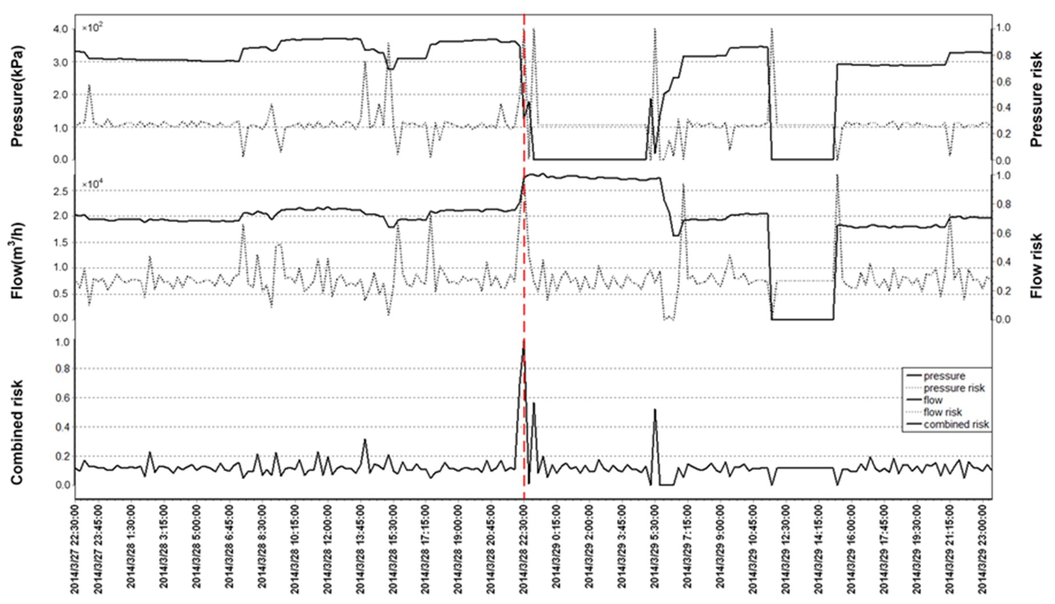
4.1.2. Two Burst Events

The monitoring data and corresponding risks before and after the bursts are presented in this section. One serious burst occurred on the night of 11 April 2014 and the other was in the early morning of 28 March 2014, as shown in Figure 12 and Figure 13.

On 11 April 2014, pressure and flow were steady before the burst occurred. The pressure fluctuation was within the range 300–350 kPa. The flow rate was maintained at 20,000 m³/h. The pressure–flow risk curve jumped sometimes as pressure and flow fluctuated, but the combined risk value remained below the red threshold because of its filtering effect. At the time of the burst (shown as the vertical dotted line), the pressure suddenly dropped to 255 kPa, and the flow increased to 27 500 m³/h. The pressure risk value was almost 1.00, and the flow risk value increased to 0.99. The combined risk value jumped to 0.99. Fifteen minutes later, workers shut down the pumps so pressure and flow abruptly dropped to 0 and the combined risk returned to the normal range.

The monitoring data for 28 March 2014 are shown in Figure 13. The pressure before the burst is about 320 kPa, and the flow is about 20,000 m³/h. Pressure and flow risk values before the burst sometimes become large because of random fluctuations in the sensors. However, the combined risk was below 0.4. When the burst occurred, the pressure dropped to 126 kPa, and the flow increased to 27,400 m³/h. At the same time, the pressure risk increased to 0.98, the flow risk became 1.00, and the combined risk increased to 0.99. After the pumps were shut down, flow and pressure sensors returned error values (extremely large values or zero). The combined risk fluctuated sharply when the burst emergency was dealt with.

In summary, the monitoring system detected two bursts from historical records based on the combined risk value. Additionally, the number of false alarms over the whole year was acceptable (i.e., at a reasonable level), which shows that this method is both feasible and reliable.

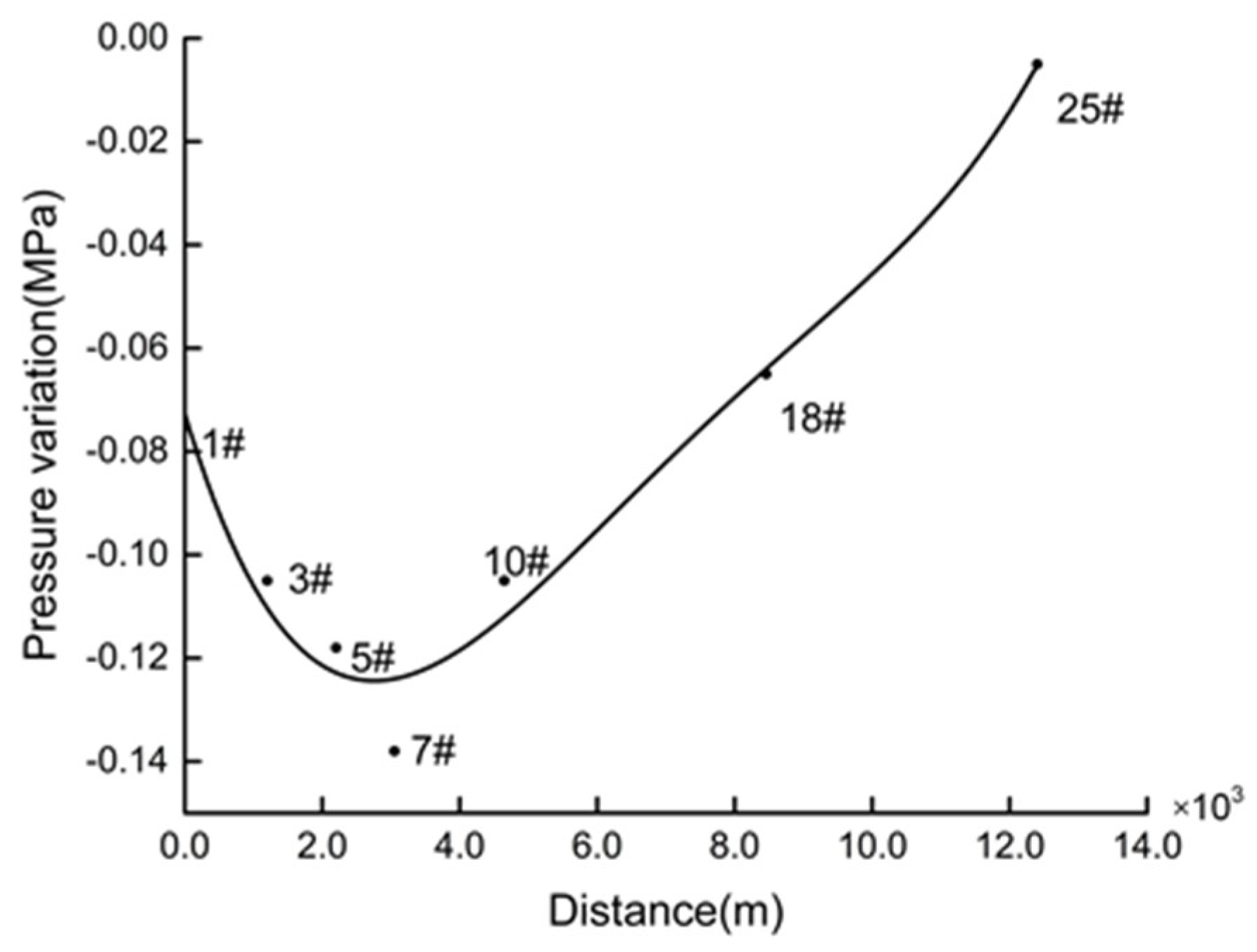
4.2. Pipe Burst Location

We selected the burst event on 11 April 2014 to evaluate the burst localization capability of our model. Pressures before and after the burst event are shown in

Table 2. Pressure change before and after the burst.

Sensor	1#	3#	5#	7#	10#	18#	25#
Pb (MPa)	0.330	0.332	0.314	0.303	0.281	0.203	0.121
Pa (MPa)	0.255	0.227	0.197	0.165	0.177	0.138	0.116
Pb − Pa (MPa)	−0.075	−0.105	−0.118	−0.138	−0.105	−0.065	−0.005
Distance from pumping station (m)	0	1200	2200	3050	4646	8459	12403

Note: P_b = pressure before the burst; P_a = pressure after the burst.

. The fitted curve of pressure change is shown in Figure 14. The absolute value of pressure change in the middle of the curve is greater than those on both sides, which makes the curve look like a funnel.

A burst is most likely to appear near the lowest point of the funnel curve, the position where the pressure drop along the pipeline reaches its maximum. In this case, the sensor showing the greatest pressure change is sensor 7. Therefore, the location of the burst was probably near sensor 7. Five sensors (sensors 1, 3, 5, 7, and 10) around the lowest point of the funnel curve are used to calculate the location of the burst. The first step is to determine parameter values. The resistance to flow parameter S and the elevation parameter C of different pipe segments were fitted (Equation (13)) and stored in the system. The burst points were calculated by Equation (15). The final results are shown in

Table 3. Estimated burst point.

Pipe Section	1–10	3–10	5–10	7–10
S × 1011 (kPa·h2/m7)	3.49	3.80	3.15	3.73
C (kPa)	−27.70	4.00	−2.67	−3.53
X (m)	2683.06	2365.52	1181.89	−1362.80
Distance from pumping station (m)	2683.06	3565.52	3381.89	1687.20

Note: For the convenience of calculation, the pressure unit is kPa and the flow unit is m³/h (cubic meter per hour) in applying Equations (13) and (15).

. The average distance from the pumping station to the burst location is 2829 m. According to the records, the burst was located near sensor 7. The difference between the calculated and actual position was <400 m. Inspectors can walk there within 5 min or drive in under 2 min, which satisfies the design requirements.

As this is a preliminary localization method for engineering use, sensors around the lowest point (i.e., the greatest pressure drop point) of the funnel curve can be chosen to estimate the burst location according to the accuracy requirements. The number of sensors and the determination of pipe sections are not limited to those shown in this case. However, the calculation accuracy would be improved if the burst location is between the two selected sensors, as shown in the fifth row of Table 3.

4.3. Parameter Sensitivity Analysis

In the burst location equation, Equation (15), the parameter S is the only parameter needed for estimation. It is fitted from the historical data. The effects of differences in S on identifying the burst location are analyzed for two selected pipe sections (1–10 and 3–10). The results are shown in

Table 4. Sensitivity analysis of parameter S.

Pipe Section	Items	S	S − 20%	S − 10%	S + 10%	S + 20%
1–10	S	3.49	2.79	3.14	3.84	4.19
	x (m)	2682.519	3355.552	2981.526	2438.018	2234.365
	Location (m)	2682.519	3355.552	2981.526	2438.018	2234.365
	Deviation (m)	0	673.033	299.007	−244.501	−448.154
3–10	S	3.80	3.04	3.42	4.18	4.56
	x (m)	2365.520	3042.988	2666.617	2119.168	1913.874
	Location (m)	3565.520	4242.988	3866.617	3319.168	3113.874
	Deviation (m)	0	677.468	301.097	−246.352	−451.646

. When S changes by 10%, the calculated position varies from 200 m to 300 m. If S changes by 20%, the location varies by about 500 m. This indicates that the parameter S is not very sensitive. However, the accuracy of S should meet the engineering design requirements. In our case, data from four different quarters are used for the estimation of S. The results show that the change of S is less than 10%, which means the error can be controlled within a reasonable range.

5. Discussion and Conclusions

The pipe burst detection and localization method proposed in this paper are derived from data observations and hydraulic principles. The resistance parameter S is insensitive, and the algorithm is simple and effective. Our experience during this study leads us to suggest the following directions for future research:

• The pressure sensors that are used for burst detection in a long-distance water transportation pipeline should be evenly distributed, and the distance between sensors should not exceed 5000 m. It is not necessary to increase the density of sensors because there would be little improvement in the results but the management costs would greatly increase.
• The sampling return period of the pressure sensors should not exceed 5 min. If the sampling time is too long, the backflow of water in the pipe after the burst point will affect the sensor readings, which will lead to large deviations in the calculations. More frequent sampling results will require more power, but will not greatly increase precision. A reasonable sampling frequency is necessary to ensure the feasibility and effectiveness of the monitoring system.
• The data fluctuations observed in a long-distance water pipeline are consistent with the behavior of a water distribution system. In practice, the accuracy of instrumental monitoring can be improved by taking account of the statistical characteristics of monitored data during normal operation of the system.

References

1. Li, R.; Huang, H.D.; Xin, K.L.; Tao, T. A review of methods for burst/leakage detection and location in water distribution systems. Water Sci. Technol.-Water Supply 2015, 15, 429–441. [Google Scholar] [CrossRef]
2. Martini, A.; Troncossi, M.; Rivola, A. Vibroacoustic Measurements for Detecting Water Leaks in Buried Small-Diameter Plastic Pipes. J. Pipeline Syst. Eng. Pract. 2017, 8, 10. [Google Scholar] [CrossRef]
3. Martini, A.; Troncossi, M.; Rivola, A.; Nascetti, D. Preliminary Investigations on Automatic Detection of Leaks in Water Distribution Networks by Means of Vibration Monitoring. Adv. Cond. Monit. Mach. Non-Station. Oper. 2014, 535–544. [Google Scholar] [CrossRef]
4. Yazdekhasti, S.; Piratla, K.R.; Atamturktur, S.; Khan, A.A. Novel vibration-based technique for detecting water pipeline leakage. Struct. Infrastruct. Eng. 2016, 13, 731–742. [Google Scholar] [CrossRef]
5. Yazdekhasti, S.; Piratla, K.R.; Atamturktur, S.; Khan, A. Experimental evaluation of a vibration-based leak detection technique for water pipelines. Struct. Infrastruct. Eng. 2018, 14, 46–55. [Google Scholar] [CrossRef]
6. Martini, A.; Troncossi, M.; Rivola, A. Leak Detection in Water-Filled Small-Diameter Polyethylene Pipes by Means of Acoustic Emission Measurements. Appl. Sci.-Basel 2017, 7, 13. [Google Scholar] [CrossRef]
7. Baghdadi, A.H.A.; Mansy, H.A. A mathematical-model for leak location in pipelines. Appl. Math. Model. 1988, 12, 25–30. [Google Scholar] [CrossRef]
8. Pudar, R.S.; Liggett, J.A. Leaks in pipe networks. J. Hydraul. Eng. 1992, 118, 1031–1046. [Google Scholar] [CrossRef]
9. Misiunas, D.; Lambert, M.; Simpson, A.; Olsson, G. Burst detection and location in water distribution networks. Effic. Use Manag. Urban Water Supply 2005, 5, 71–80. [Google Scholar] [CrossRef] [Green Version]
10. Lee, P.J.; Vitkovsky, J.P.; Lambert, M.F.; Simpson, A.R.; Liggett, J.A. Leak location using the pattern of the frequency response diagram in pipelines: A numerical study. J. Sound Vib. 2005, 284, 1051–1073. [Google Scholar] [CrossRef] [Green Version]
11. Bicik, J.; Kapelan, Z.; Makropoulos, C.; Savic, D.A. Pipe burst diagnostics using evidence theory. J. Hydroinform. 2011, 13, 596–608. [Google Scholar] [CrossRef] [Green Version]
12. Srirangarajan, S.; Allen, M.; Preis, A.; Iqbal, M.; Lim, H.B.; Whittle, A.J. Wavelet-based burst event detection and localization in water distribution systems. J. Signal Process. Syst. Signal Image Video Technol. 2013, 72, 1–16. [Google Scholar] [CrossRef]
13. Mounce, S.R.; Machell, J. Burst detection using hydraulic data from water distribution systems with artificial neural networks. Urban Water J. 2006, 3, 21–31. [Google Scholar] [CrossRef]
14. Farley, B.; Mounce, S.R.; Boxall, J.B. Development and field validation of a burst localization methodology. J. Water Resour. Plan. Manag. 2013, 139, 604–613. [Google Scholar] [CrossRef]
15. Mounce, S.R.; Boxall, J.B.; Machell, J. Development and verification of an online artificial intelligence system for detection of bursts and other abnormal flows. J. Water Resour. Plan. Manag.-ASCE 2010, 136, 309–318. [Google Scholar] [CrossRef]
16. Ye, G.L.; Fenner, R.A. Kalman filtering of hydraulic measurements for burst detection in water distribution systems. J. Pipel. Syst. Eng. Pract. 2011, 2, 14–22. [Google Scholar] [CrossRef]
17. Choi, D.Y.; Kim, S.W.; Choi, M.A.; Geem, Z.W. Adaptive Kalman filter based on adjustable sampling interval in burst detection for water distribution system. Water 2016, 8, 142. [Google Scholar] [CrossRef]
18. Ye, G.; Fenner, R.A. Weighted least squares with expectation-maximization algorithm for burst detection in U.K. water distribution systems. J. Water Resour. Plan. Manag. 2014, 140, 417–424. [Google Scholar] [CrossRef]
19. Lin, C.C. A hybrid heuristic optimization approach for leak detection in pipe networks using ordinal optimization approach and the symbiotic organism search. Water 2017, 9, 812. [Google Scholar] [CrossRef]
20. Wu, Y.P.; Liu, S.M.; Wu, X.; Liu, Y.F.; Guan, Y.S. Burst detection in district metering areas using a data driven clustering algorithm. Water Res. 2016, 100, 28–37. [Google Scholar] [CrossRef] [PubMed]
21. Wu, Y.P.; Liu, S.M. A review of data-driven approaches for burst detection in water distribution systems. Urban Water J. 2017, 14, 972–983. [Google Scholar] [CrossRef]
22. Zhao, D.D.; Cheng, W.P. Study on minimum detectable pipe diameter for pipe burst in water distribution system. China Water Wastewater 2014, 30, 117–122. (in Chinese). [Google Scholar]
23. Shafer, G.A. A Mathematical Theory of Evidence; Princeton University Press: Princeton, NJ, USA, 1976. [Google Scholar]
Figure 1. Diagram of a water delivery pipeline.
Water 10 01727 g001
Figure 2. Four states of change in pressure and flow.
Water 10 01727 g002
Figure 3. Pressure–flow curve of pumping station.
Water 10 01727 g003
Figure 4. Pressure (a) and flow (b) at the pump station.
Water 10 01727 g004
Figure 5. Histograms of (a) pressure and (b) flow fluctuations at the pumping station.
Water 10 01727 g005
Figure 6. Cumulative probability curves of (a) pressure and (b) flow fluctuations at the pumping station.
Water 10 01727 g006
Figure 7. Pressure variation along the pipe.
Water 10 01727 g007
Figure 8. Diagram of a pipe section.
Water 10 01727 g008
Figure 9. Layout of pipelines.
Water 10 01727 g009
Figure 10. Pipe burst monitoring web page.
Water 10 01727 g010
Figure 11. Flowchart of pipe burst monitoring system.
Water 10 01727 g011
Figure 12. Burst risk on 11 April.
Water 10 01727 g012
Figure 13. Burst risk on March 28.
Water 10 01727 g013
Figure 14. Pressure change after the burst.
Water 10 01727 g014