Abstract
Generic habitat suitability criteria (HC) are often developed from spatially and temporally variable hydroecological datasets to increase generality, cost-effectiveness, and time-efficiency of habitat models. For benthic macroinvertebrates (BMIs), however, there is no prior knowledge on the spatiotemporal variation in their habitat preferences and how this may be reflected in the final environmental flow (e-flow) predictions. In this study, we used a large, spatiotemporally variable BMI-hydroecological dataset and developed generic, local, and season-specific subsets of HC for three seasons and two river types within various data pre-treatment options. Each subset was used to train a fuzzy habitat model, predict the habitat suitability in two hydrodynamically-simulated river reaches, and develop/compare model-based e-flow scenarios. We found that BMIs shift their habitat preferences among seasons and river types; consequently, spatiotemporally variable e-flow predictions were developed, with the seasonal variation being greater than the typological one. Within this variation, however, we found that with proper data pre-treatment, the minimum-acceptable e-flows from the generic models mostly (65–90%) lay within the acceptable e-flows predicted by the local and season-specific models. We conclude that, within specific limitations, generic BMI-HC can be used for geographically extended, cost-effective e-flow assessments, compensating for the within-limits loss of predictive accuracy.
1. Introduction
Spatiotemporal variation has long been a subject of discussion in physical habitat modelling [1,2,3,4,5,6,7]. From a management-oriented perspective, the use of multiple local and season-specific habitat suitability criteria to develop model-based environmental flow recommendations is considered unrealistic [2,3]; usually, the costs and time required to generate site- and season-specific habitat preferences cannot be covered by the limited funding available and, thus, the ability to develop appropriate local hydroecological datasets is also limited [3]. Research, however, suggests that aquatic organisms often shift their habitat preferences among seasons and may have different requirements in different geographical locations. This has been repeatedly confirmed for fish, as there is a complete agreement between studies on different species and from different regions [1,8,9,10,11], and thus, in fish-based studies, site- and season-specific habitat suitability criteria have been preferred over generic ones [12,13]. In contrast, the fewer available studies on benthic macroinvertebrates (BMIs) reach contrasting conclusions; although most studies suggest increased performance of habitat models when local and season-specific criteria are applied [4,5,11,14], others conclude that the observed differences are not significant enough to inhibit the application of generic habitat suitability criteria [2,3,15]. However as Kelly et al. indicate [14], ‘some balance needs to be found between generality and specificity’ to widen the applicability of model-based environmental flow assessments.
Typically, habitat preference datasets consist of microhabitat samples relating the flow velocity (V), the water depth (D) and the type of substrate (S) with a habitat suitability value, calculated either by using the abundance of target aquatic organisms or by applying traits- or metrics-based approaches. These preferences are often visualized in the two-dimensional space as habitat suitability curves [4,16,17] but other approaches have been also implemented [18,19,20]. The habitat preference datasets are then used as training data in hydraulic habitat models, that is, the reference data which will be used by the model to predict the habitat suitability (Κ) in samples/microhabitats with known V, D, and S values and unknown Κ. Currently, there are various alternatives available for the development of habitat suitability criteria, reflecting the aforementioned challenging effort to balance the sources of error and variation towards cost-effectiveness and time-efficiency. In this effort, hydroecological data from geographically and hydrologically various river types and in different time periods, often collected within different projects, are either treated separately to develop site- and season-specific criteria or are aggregated to increase sample size and/or extend the geographical and typological applicability of a model [21,22,23]. In BMI-based studies, typical aggregation schemes include spatiotemporal pooling-of samples from different sites and/or seasons-without pre-treatment [17,24]; spatial aggregation of samples only from specific, usually low-flow periods [25,26]; and spatiotemporal pooling of samples after proper pre-treatment [4,19,27].
Although it has been previously acknowledged that spatial and temporal variation may result in error and uncertainty in model-based environmental flow predictions [28,29], case studies including and quantifying this spatiotemporal component are currently missing. Do benthic macroinvertebrates shift their habitat preferences among seasons and in different geographical locations? Will a model-based environmental flow assessment reach similar prediction by applying local and season-specific-versus generic habitat suitability criteria? Are the possible differences in the predictions variable enough to inhibit the application of generic habitat suitability criteria? Can a generic dataset be treated appropriately to enable its use in multiple locations? These questions have not been properly addressed due to the lack of relevant comparative assessments, but within the context of ‘trading-off between modelling accuracy and generality’ [30], such assessments are necessary to properly guide future habitat modelling efforts.
The purpose of this study was (i) to explore the possible seasonal and typological variation in the habitat preferences of benthic macroinvertebrates and (ii) to investigate whether this spatiotemporal variation can be—at least partially—omitted to facilitate the development of generic BMI habitat suitability criteria. Based on a large BMI-hydroecological dataset collected from Greek streams and rivers, we developed local and generic habitat suitability criteria for benthic macroinvertebrates, including (i) three seasons, (ii) two river types, and (iii) five Κ-calculation alternatives. With the application of a two-dimensional hydrodynamic habitat model, we used these criteria to develop model-based environmental flow predictions in two river reaches in Greece. Our ultimate goal was to calculate the probability of agreement between the environmental flow predictions based on the different habitat suitability criteria. Low probability would suggest that local and season-specific habitat suitability criteria cannot be replaced by generic ones due to the high loss in the model’s predictive accuracy. High probability of agreement would suggest that generic habitat suitability criteria can be used in model-based EFAs within the concept of balancing between a model’s predictive performance, generality, cost-effectiveness, and time-efficiency.
2. Materials and Methods
2.1. Overview of the Analysis
The steps followed to implement our analysis are outlined below:
- Development-acquisition of a benchmark microhabitat preference dataset.
- Calculation of habitat suitability (κ) for each microhabitat sample using BMI metrics.
- Normalization of κ in the 0–1 scale, using five alternatives-options.
- Training of a habitat model using each of the five κ-normalization options within three seasons and two river types.
- Application of hydrodynamic simulations in two river reaches to acquire V and D values in multiple discharges.
- Prediction of κ in the two reaches using the various training alternatives (subsets).
- Development of spatially and temporally varying environmental flow scenarios, comparisons and discussion on the selection of the minimum acceptable and optimal environmental flows within the various subsets.
2.2. Development/Acquisition of a Benchmark Microhabitat Preference Dataset
The habitat preferences of benthic macroinvertebrates were acquired from the benthos-GR dataset (https://github.com/chtheodoro/benthos-GR) [18], consisting of 380 microhabitat samples collected from 9 reference (unpolluted) sites in Greece (max. 20 microhabitats per site) (see Table S1 for the complete BMI taxalist). The dataset spans three seasons (spring, summer, and autumn of 2015) and three river types, based on Van de Bund [31], (i) RM-1 (10–100 km2, altitudes between 200–800 m a.s.l., mixed geology), (ii) RM-2 (100–1000 km2, altitude < 600 m a.s.l., mixed geology), and (iii) RM-4 (10–1000 km2, altitudes between 400–1500 m a.s.l., mixed geology). Each sample, delineated as a 0.25 × 0.25 m2 rectangular area, relates V, D, and S to a habitat suitability value calculated using commonly applied BMI-community metrics [32,33,34,35] (No. of families, Shannon-Wiener’s diversity index, No. of Ephemeroptera-Plecoptera-Trichoptera families, total community abundance). As the samples from RM-1 and RM-2 types were disproportionately lower than the RM-4 samples, they were merged to a single RM1-2 category including middle and lowland sites with medium-sized catchments, in contrast to the smaller-catchment, highland sites of the RM4 type. Thus, the number of microhabitat samples per season and per river type in the dataset (n) were (i) spring samples (n = 160), (ii) summer samples (n = 160), (iii) autumn samples (n = 60), (iv) RM1-2 samples (n = 100), (v) RM4 (n = 280) (Figure 1). Two-dimensional representations (scatterplots) of the hydroecological relationships between the abiotic predictors (V, D, S) and the selected BMI metrics are shown in the Appendix A (Figure A1, Figure A2, Figure A3, Figure A4 and Figure A5).
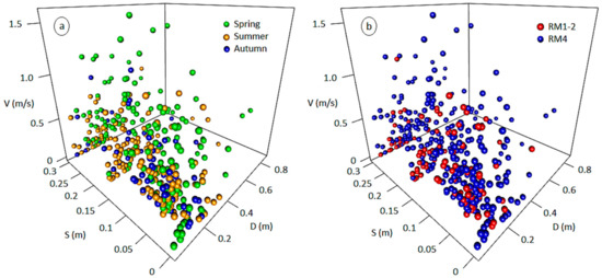
Figure 1.
Three-dimensional representation of the 380 microhabitat samples of the benthos-GR dataset spanning three seasons (a) and two river types (b). V: flow velocity, D: water depth, S: substrate type.
2.3. Calculation of Habitat Suitability Using BMI Metrics
As detailed in Theodoropoulos et al. [18], for the calculation of habitat suitability, each of the aforementioned metrics was weighted based on a combination of expert-judgment and previous literature [32,33,34,35,36] to reflect its relevant contribution-significance, and the final, unnormalized κ has been calculated as follows:
where is the unnormalized habitat suitability of the ith microhabitat; denotes the number of BMI taxa (families) found at the ith microhabitat; denotes the Shannon’s diversity index for the ith microhabitat; is the number of EPT taxa found at the ith microhabitat; is the abundance of benthic macroinvertebrates found at the ith microhabitat.
As the unnormalized κ values arbitrarily ranged from 0 to higher than 3000, and in accordance with previous literature on the calculation of K [16,36,37,38,39], a normalization process was afterwards applied to scale the κ values to the 0–1 range. Correlations between the abiotic predictors and the selected BMI metrics are shown in the Appendix A (Table A1).
2.4. Normalization of κ in the 0–1 Scale, Using Five Alternatives
We applied five alternatives to normalize the unnormalized habitat suitability values:
- The unnormalized habitat suitability values are divided by the maximum κ observed at the whole dataset (seasonal and typological variation not accounted; no seasonal grouping, no typological grouping applied—hereafter called maxall).
is the normalized habitat suitability of the ith microhabitat ranging from 0 to 1; denotes the number of BMI taxa (families) of the ith microhabitat; denotes the Shannon’s diversity index for the ith microhabitat; is the number of EPT taxa found at the ith microhabitat; is the abundance of benthic macroinvertebrates of the ith microhabitat; denotes the maximum unnormalized habitat suitability value observed in the whole dataset.
- 2.
- The unnormalized habitat suitability values are divided by the maximum κ observed at each season (seasonal variation; no typological grouping applied—hereafter called maxseason).
is the normalized habitat suitability of the ith microhabitat at the nth season, ranging from 0 to 1; denotes the number of BMI taxa (families) found at the ith microhabitat at the nth season; denotes the Shannon’s diversity index for the ith microhabitat of the nth season; is the number of EPT taxa found at the ith microhabitat at the nth season; is the abundance of benthic macroinvertebrates of the ith microhabitat at the nth season; denotes the maximum unnormalized habitat suitability value observed at the nth season.
- 3.
- The unnormalized habitat suitability values are divided by the maximum κ observed at each river type (typological variation; no seasonal grouping applied—hereafter called maxtype).
is the normalized habitat suitability of the ith microhabitat of the pth river type, ranging from 0 to 1; denotes the number of BMI taxa (families) found at the ith microhabitat of the pth type; denotes the Shannon’s diversity index for the ith microhabitat of the pth type; is the number of EPT taxa found at the ith microhabitat of the pth type; is the abundance of benthic macroinvertebrates found at the ith microhabitat of the pth type; denotes the maximum unnormalized habitat suitability value observed of the pth type.
- 4.
- The unnormalized habitat suitability values are divided by the maximum κ observed at each site at each season (seasonal and typological grouping—hereafter called maxsite).
is the normalized habitat suitability of the ith microhabitat at the jth site at the nth season ranging from 0 to 1; denotes the number of BMI taxa (families) of the ith microhabitat at the jth site at the nth season; denotes the Shannon’s diversity index for the ith microhabitat of the jth site at the nth season; is the number of EPT taxa found at the ith microhabitat of the jth site at the nth season; is the abundance of benthic macroinvertebrates of the ith microhabitat at the jth site at the nth season; denotes the maximum unnormalized habitat suitability value observed at the jth site at the nth season.
- 5.
- The value of each metric is divided by the maximum value of this metric observed at each site at each season (seasonal and typological grouping—hereafter called maxmetric).
is the normalized habitat suitability of the ith microhabitat at the jth site at the nth season ranging from 0 to 1; denotes the maximum number of BMI taxa (families) of the jth site at the nth season; denotes the maximum Shannon’s diversity index of the jth site at the nth season; is the maximum number of EPT taxa found at the jth site at the nth season; is the maximum abundance of benthic macroinvertebrates of the jth site at the nth season.
2.5. Training of a Habitat Model Using Each of the Five κ-Normalization Options within Three Seasons and Two River Types
A fuzzy rule-based Bayesian algorithm (FRB) based on Brookes et al. [40], detailed in Theodoropoulos et al. [18] and implemented in the HABFUZZ software [41] was trained and cross-validated (see Supplementary Material—Table S2 for details). In brief, the FRB algorithm applies a fuzzification process to convert the numerical input values of V and D to membership degrees (MDs) in overlapping, trapezoidal-shaped fuzzy sets [19] (Table 1). By this process, each numerical input is assigned to one or more fuzzy sets with a MD ranging from zero to one; K values are also classified in five classes (0 ≤ bad ≤ 0.2; 0.2 < poor ≤ 0.4; 0.4 < moderate ≤ 0.6; 0.6 < good ≤ 0.8; 0.8 < high ≤ 1). The training dataset (in this case the multiple alternatives of the benthos-GR dataset), with a priori calculated K values, is used to develop sets of data-driven IF-THEN rules (Table S2), relating the simultaneous occurrence of a series of fuzzy sets to a specific K class. The fuzzy MD of each input is afterwards accounted as the probability of occurrence of the particular fuzzy set, such as ‘IF V is low with a MD of 1 AND D is moderate with a MD of 1 AND S is gravel with a MD of 1 THEN K is good with a MD of 0.3 and moderate with a MD of 0.7’. The IF-THEN rules are then combined using the Bayesian joint probability, so that (referring to the previous example) the probability of the specific microhabitat’s K being good is the joint probability that V is low AND D is moderate AND S is gravel AND K is good (1 × 1 × 1 × 0.3 = 0.3), while the probability of K being moderate is the joint probability that V is low AND D is moderate AND S is gravel AND K is moderate (1 × 1 × 1 × 0.7 = 0.7). Based on a utility function [18,40], a score is assigned at each K class (bad: 0.1; poor: 0.3; moderate: 0.5; good: 0.7; high: 0.9) and the habitat suitability for each microhabitat is predicted using the following equation:
where, is the predicted habitat suitability; denotes the joint probability of occurrence of each κ class; denotes the score of each κ class; For the previous example, equals to 0.7 × 0.5 + 0.3 × 0.7 = 0.56.

Table 1.
Class names and relevant class parameters of the hydraulic variables. Substrate type (S) and habitat suitability (K) were treated as crisp (not fuzzy) sets. V: flow velocity; D: water depth.
The predicted K value is then compared with the K observed in the training dataset for the specific microhabitat and the predictive accuracy of the algorithm is estimated within a three-K-class system (low: 0–0.2; moderate: 0.2–0.6; acceptable: 0.6–1) (Table S2), using a 10-fold cross-validation process [42]: The initial dataset is randomly partitioned in ten equal-sized subsamples. Nine subsamples are used as the training dataset and the remaining subsample is used for model validation. This process is repeated ten times (folds), using a different subsample for validation at each iteration. The performance of each model is evaluated as the average percentage of the correctly classified instances (%CCI) between each iteration of the ten-fold cross-validation process (Appendix A—Figure A6 and Figure A7).
2.6. Hydrodynamic Simulation of Two River Reaches to Acquire V, D and S Values in Multiple Discharges (Q)
Topographic data (longitude, latitude, bottom elevation) and hydrometric data (Q, V and D at randomly selected points in two different discharges), were recorded in two river reaches in Greece (Parapeiros River and Oinoi Stream-Figure 2) at multiple sampling campaigns. The Blue Kenue software [43] was used to construct a triangulated computational mesh for each river reach based on the relevant topographic information (Parapeiros-reach mesh properties: 277-m long; 9875 elements; 5170 nodes, Oinoi-reach grid properties: 370-m long; 7140 elements; 3938 nodes). The TELEMAC 2D hydrodynamic model (Electricité de France, Paris, France) [44] was afterwards used to simulate V and D values at each node of each computational mesh in multiple discharges (11 Q scenarios for the Parapeiros reach and 16 Q scenarios for the Oinoi reach). The models were calibrated-validated as follows: initial values for the Manning’s roughness coefficient (n) were acquired from the tables given in Chow [45] through an on-site visual estimation of the major types of substrate at each reach. The n values were afterwards properly adjusted within multiple model runs until an acceptable agreement was observed between the field-recorded and the simulated values of V and D at each of the randomly selected points at each river reach. The models were calibrated in the lower discharges and validated in the higher discharges. As this study is focused on habitat modelling, for further details on the hydrodynamic simulations of the Parapeiros and Oinoi reaches, please refer to [23,46], respectively.
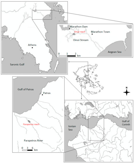
Figure 2.
The Parapeiros River and Oinoi Stream where the relevant reaches were hydrodynamically simulated.
2.7. Prediction of K in the Two Test Reaches Using the Various Training Alternatives
Within the process mentioned in Section 2.4, we developed 20 training alternatives (subsets) to explore the seasonal and typological variation in the BMI habitat preferences and the relevant variation in the selection of the minimum acceptable and optimal environmental flow scenario within each subset (Figure 3).
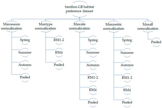
Figure 3.
Seasonal and typological subsets of the benthos-GR dataset developed within the various κ-normalization methods. In total, 20 subsets were developed and 20 environmental flow assessments were applied at each test case, using each subset as a training dataset for the habitat model.
As it is obvious, not all normalization alternatives can be used in all cases. For example, since in the maxall option, the κ values are divided by the maximum observed κ at the whole benthos-GR dataset, the maxall option cannot be applied only for the spring (or only for the RM4) samples; in contrast, the maxseason, maxsite, and maxmetric options can be applied in a seasonal subset, and likewise, the maxtype, maxsite, and maxmetric options can be applied in a typological subset. Each of the aforementioned 20 subsets was used as a training dataset in the HABFUZZ habitat model, based on which the integrated TELEMAC 2D + HABFUZZ model predicted K at each node of each computational mesh according to the V, D, and S values simulated by TELEMAC 2D at each discharge. In total, the K values in 540 discharge scenarios were simulated; 20 subsets × 11 Q scenarios for the Parapeiros reach and 20 subsets × 16 Q scenarios for the Oinoi reach.
2.8. Development of Environmental Flow Scenarios
Similarly to the fish-based ‘Weighted Usable Area’ approach of Bovee [16], to advance from the microhabitat scale to the reach scale, the K multimetric index (microhabitat scale) was combined with abiotic metrics describing habitat connectivity, habitat availability, and the percentage of wetted nodes, within the Optima Flow Scenario (OFS) index (reach scale) as follows:
- Overall Suitability Index (OSI):
- Normalized OSI (nOSI):
where Ki (from 0 to 1) denotes the habitat suitability at each node of the computational grid; w denotes the total No. of wetted nodes in the computational grid at each Q scenario.
- 3.
- Certainty of prediction (COP): The ratio of the No. of microhabitat combinations actually found in the training dataset to the total No. of nodes in the computational mesh; instead of requiring the user’s interference to manually adjust the missing fuzzy rules, HABFUZZ is completely data-driven and when a microhabitat combination is not found in the training dataset, instead of returning some arbitrary K value for a particular node (e.g., −1), it uses the K value of its neighboring node in the mesh, with a simultaneous assessment of the relevant prediction error.
- 4.
- Percentage of wetted nodes in the computational mesh at each Q scenario (w).
- 5.
- Habitat connectivity (C): The ratio of connected (neighboring) nodes with K > 0.6 to the total number of wetted nodes with K > 0.6.
- 6.
- Habitat availability (A): The ratio of connected (neighboring) nodes with K > 0.6 to the total number of nodes in the study reach (wetted and dry).
All values were normalized in a 0–1 scale by dividing each with the maximum OFS observed. Based on the status classification system introduced in the Water Framework Directive 2000/60/EC [47], all Q scenarios with OFS values higher than 0.6 were considered acceptable as environmental flows; Seasonal and typological comparisons were applied based on the minimum and optimal environmental flow predictions to ultimately explore the variation of the different environmental flow scenarios developed by the various subsets, corresponding to spatially and temporally different habitat suitability criteria.
3. Results
The seasonal and typological OFS means and standard deviations (SD) within the various κ-normalization alternatives (see Table A2, Table A3, Table A4 and Table A5 for the actual mean and SD values), along with the OFS values for each discharge simulated in the various seasons and river types, are depicted in Figure 4, Figure 5 and Figure 6 for the Parapeiros reach and in Figure 7, Figure 8 and Figure 9 for the Oinoi reach. Two trends are evidenced in both reaches:
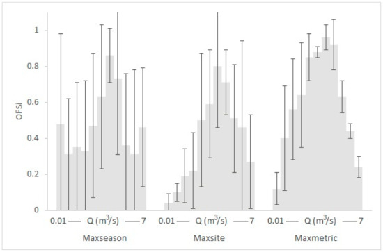
Figure 4.
Graphical representation of the Seasonal optimal flow scenario (OFS) means (grey shaded) and standard deviations within the various κ-normalization alternatives for the Parapeiros reach. The OFS values of spring, summer and autumn for each discharge (Q) have been averaged.
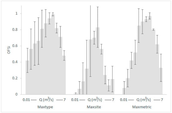
Figure 5.
Graphical representation of the typological OFS means (gray shaded) and standard deviations within the various κ-normalization alternatives for the Parapeiros reach. The OFS values of RM1-2 and RM4 types for each discharge (Q) have been averaged.
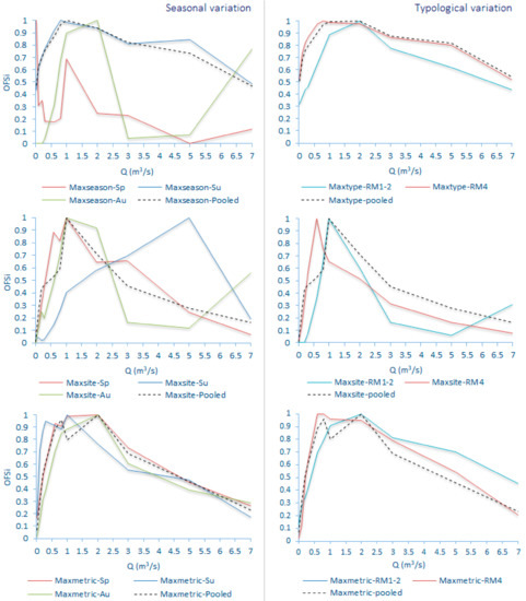
Figure 6.
Seasonal and typological variation in the selection of the OFS for the Parapeiros reach within the various habitat-suitability calculation-normalization options (Sp: Spring; Su: Summer; Au: Autumn).
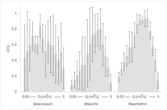
Figure 7.
Graphical representation of the seasonal OFS means (gray shaded) and standard deviations within the various κ-normalization alternatives for the Oinoi reach. The OFS values of spring, summer and autumn for each discharge (Q) have been averaged.
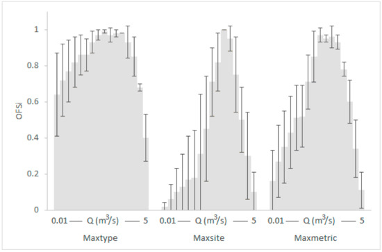
Figure 8.
Graphical representation of the typological OFS means (gray shaded) and standard deviations within the various κ-normalization alternatives for the Oinoi reach. The OFS values of RM1-2 and RM4 types for each discharge (Q) have been averaged.
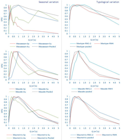
Figure 9.
Seasonal and typological variation in the selection of the optimal flow scenario (OFS) for the Oinoi reach within the various habitat-suitability calculation-normalization options (Sp: Spring; Su: Summer; Au: Autumn).
- The seasonal differences in the OFS values for the same Q within the various subsets were greater and more variable than the relevant typological differences. For example, in the Parapeiros reach, the OFS value for Q = 0.3 m3/s was 0.18 in spring, 0.77, in summer and 0.04 in autumn (mean: 0.33; SD: 0.39; maxseason normalization). For the same Q, the OFS value for the RM1-2 type was 0.46 and for the RM4 type was 0.86 (mean: 0.66; SD: 0.29; maxtype normalization). In the Oinoi reach, the OFS value for Q = 0.05 m3/s was 0.91 in spring, 0.61 in summer, and 0.26 in autumn (mean: 0.59; SD: 0.33; maxseason). For the RM1-2 type, the OFS for Q = 0.05 m3/s was 0.89, and for the RM4 type it was 0.65 (mean: 0.77; SD: 0.17; maxtype).
- The observed seasonal and typological variation decreased when site-based or metric-based normalizations were applied (maxsite and maxmetric, respectively) with the maxmetric option mostly showing the lowest variation among seasons and river types. In the seasonal comparisons of the Parapeiros reach, the maxmetric option had the lowest OFS-SD for all Q values (100% lower SD) when compared with the maxseason option and for 7 out of 11 discharges (64%) when compared with the maxsite option. In the relevant typological comparisons, the maxmetric option showed 81% lower SD, in comparison with the maxtype option and 64% lower SD when compared with the maxsite option. The seasonal comparisons for the Oinoi reach showed that the SD for the maxmetric option was 81% lower (13 out of 16 Q values) when compared with both the maxseason and maxsite alternatives. The relevant typological comparisons however, showed only 31% lower SD values (5 out of 16 Q values) in comparison with the maxtype option. The comparison between the maxsite and maxmetric options, once again showed 68% lower SD for the maxmetric normalization.
When comparing the seasonal and typological differences in the prediction of the minimum acceptable environmental flows (OFS > 0.6) within the various κ-normalization options, it can be seen that the predictions were highly variable; for the Parapeiros reach (Figure 10), the minimum acceptable environmental flow varied from 0.01 m3/s (maxseason—spring) to 2 m3/s (maxsite—summer). For the Oinoi reach (Figure 11) the minimum environmental flow varied from 0.01 m3/s (maxseason—spring; maxtype—RM1-2) to 0.9 m3/s (maxsite—RM4).
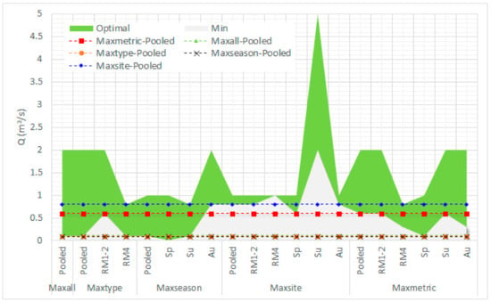
Figure 10.
Overall comparison on the selection of the minimum acceptable and optimal environmental flow in the Parapeiros River between the various habitat-suitability calculation-normalization options including seasonal and typological variation (Sp: Spring; Su: Summer; Au: Autumn). Predictions within the green area are considered acceptable (lying between the minimum and optimal environmental flows).
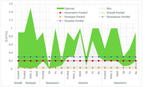
Figure 11.
Overall comparison on the selection of the minimum acceptable and optimal environmental flow in the Oinoi Stream between the various habitat-suitability calculation-normalization options including seasonal and typological variation (Sp: Spring; Su: Summer; Au: Autumn). Predictions within the green area are considered acceptable (lying between the minimum and optimal environmental flows).
It must be noted that, within this variation, when environmental flows are predicted by pooling all seasons and types under the various κ-normalization options, the minimum environmental flows predicted within the maxsite and maxmetric alternatives in both reaches, mostly lay within the acceptable environmental flows predicted by all other options (hereafter called between-models’ degree of agreement—DoA), in contrast to the other training alternatives (maxseason, maxtype, maxall). In the Parapeiros reach, maximum DoA was reached by pooling the dataset within the maxsite option (90%; within acceptable limits in 18 out of the 20 predictions). The maxmetric option showed 65% DoA and all other alternatives had 35% agreement. In the Oinoi reach, the maxsite option showed again maximum agreement (90%), with the maxmetric, maxseason, maxall, and maxtype options showing 75%, 75%, 30%, and 15% DoA, respectively.
4. Discussion
4.1. Seasonal and Temporal Variation in the Habitat Preferences of Benthic Invertebrates
The results of the study suggest that benthic macroinvertebrates shift their habitat preferences among seasons and in different geographical locations, with the seasonal shifts being greater than the typological ones (the between-seasons SD values were constantly higher than the between-types SD). During summer, benthic invertebrates preferred faster-flowing and deeper habitats (the relevant habitat suitability peaked at higher discharges, reflecting higher V and D values). During spring and autumn, their preferences were more variable, but in general, a preference for shallower and slow-flowing habitats was observed, with the habitat suitability peaking at the lowest discharges mostly in spring. Although seasonal differences in macroinvertebrate-community abundance and composition have long been reported in literature [48,49,50,51,52], community-shifts in their habitat preferences have not been studied; we assume that such ‘shifting behavior’ may be associated with the seasonal fluctuation of environmental variables, which are known primary drivers of BMI-community changes, that is, shading, water temperature and dissolved oxygen [53]. As summer approaches, shading from the surrounding riparian vegetation is reduced, the water temperature increases, the dissolved oxygen concentration decreases [54] and consequently, faster flowing, deeper, better oxygenated habitats provide shelter against the changing environment. In contrast to the under-studied seasonal shifts, typological differences in the habitat preferences of BMIs have been previously documented, suggesting a preference for shallower water depths and lower velocities in smaller rivers [15,55]. Our results also confirm this trend; the habitat suitability in the RM1-2 type, which includes mid- and lowland sites draining larger catchments, peaked at higher discharges, reflecting a BMI preference for higher velocities and water depths, in comparison to the RM4 type consisting of highland sites with small-sized catchments.
4.2. Seasonal and Typological Variation in the Environmental Flow Predictions within the Various κ-Normalization Options
As it was expected, the seasonal and typological variation in the habitat suitability of benthic macroinvertebrates was highly reflected in the minimum acceptable and optimal model-based environmental flow (e-flow) predictions. E-flow recommendations based on habitat suitability criteria developed from spring samples only, were slightly or highly different than e-flow recommendations based on habitat suitability criteria developed from summer or autumn samples of the same set of sites (maxseason option-Figure 6 and Figure 9). The same trend, but with smaller differences, was observed with the use of habitat suitability criteria from different river types (maxtype option—Figure 6 and Figure 9). This suggests that local and season-specific habitat criteria should be used to increase predictive accuracy-it also confirms most previous BMI-based studies (but see [56])—accounting for the observed spatial and temporal variation [4,5,11,14].
However, despite the observed and acknowledged spatiotemporal variation, two key-findings of our study support the use of generic habitat suitability criteria after proper data pre-treatment: (i) among the various κ-normalization options, the maxmetric option significantly reduced the observed seasonal and typological variation (maxmetric-Figure 6 and Figure 9), thus being a potential candidate for generic applications; (ii) when the habitat suitability values in the reference dataset were normalized per site or per metric (maxsite and maxmetric options, respectively) the final environmental flow predictions mostly lay within the acceptable environmental flows range predicted by all other options. This means that such a generic-criteria-based assessment will have a high probability, ranging from 65% (maxmetric) to 90% (maxsite) to develop environmental flow recommendations, which will finally benefit the benthic-invertebrate community. Similarly to the majority-vote approach commonly followed in machine-learning algorithms, all models, either season- or type-specific, agreed-voted that the minimum acceptable e-flow predictions developed by pooling all samples, pre-treated using the maxsite and maxmetric options were also acceptable (though not minimum) by the other models (Figure 10 and Figure 11). The fact that this trend was observed twice in this study (for both river reaches studied) leads us to assume that it was not due to chance but future studies are of course required to either further confirm or disprove the aforementioned trend. The use of generic habitat suitability criteria has also been suggested by the results of Komínková et al. [56], which showed only 10% seasonal variation in their BMI-based e-flow predictions for an urban creek, with the seasonal, minimum-acceptable e-flows being almost equal.
4.3. Issues to Be Considered in Spatiotemporal Pooling of Hydroecological Data
Habitat models predict complex distributional patterns based on a reduced set of predictor variables [28]. Due to the stochastic nature of hydroecological data [57], mismatches between the models’ prediction and the actual observed are inevitable; spatiotemporal pooling of hydroecological data has been considered as an additional source of prediction error [28]. The benefits and limitations of spatiotemporal pooling have long been discussed in literature and despite the multitude of data-mining methods, research on the development of robust data-mining applications is still ongoing [58]. Our study, inter alia, confirmed the aforementioned, showing varying results in many internal aspects of the habitat modelling process, which should be taken into account when spatiotemporal pooling of hydroecological data is attempted:
- The fuzzy rules developed from the various κ-normalization options were very different; the habitat suitability class for the same microhabitat combination varied from bad to high (Table S2), reflecting the importance of the normalization process (seasonal, typological, site- or metric-based). Theoretically, normalizing a spatially variable dataset, that includes multiple river types, only by season, does not take into account the geographical-typological variation. Normalizing a temporally variable dataset, that includes multiple seasons, only by type, does not take into account the seasonal variation. The very low environmental flow values (0.01 m3/s) predicted by the seasonal models are possibly indicative of a relevant inadequacy of these κ-normalization options. We assume that a per-site or per-metric normalization could partially account for both seasonal and typological variation, but in the absence of a field-validation for our models (they were cross-validated but not field-validated), we can currently only discuss the within-models-agreement trends on the final environmental flow prediction.
- Low sample sizes often resulted in decreased cross-validation accuracy; this was evident by the %CCI values of the autumn samples (n = 60; Figure A6 and Figure A7), which were the lowest observed within the various models developed, varying from 46% to 52%. The current FRB algorithm requires 5 × 5 × 8 = 200 fuzzy rules to adequately predict the habitat suitability (although not all rules may be necessary, for example, a microhabitat combination of very high V and very deep D will rarely be observed in a river reach). Thus, a small dataset will be inherently incapable of providing the observations required to develop an effective rules-database [28]. As the sample size increases however, more microhabitat combinations will be included, the fuzzy-rules database will increase, and the model’s performance is also expected to increase [59,60].
4.4. Can We Use Generic Instead of Local and Season-Specific Habitat Suitability Criteria?
Before answering, it must be noted that the comparisons applied in our study included typologically different sites, but of similar hydromorphological and hydraulic properties, that is, flow velocities ranging from 0 m/s to 1.2 m/s, water depths ranging from 0.01 m to 1 m and substrate types consisting mainly of boulders, cobbles, pebbles, and gravel. It is obvious that the application of generic habitat suitability criteria from these sites in rivers with completely different hydromorphology (e.g., deep, slow-flowing habitats composed of sand and silt) is prohibitive.
The results of our study clearly showed spatial and temporal shifts in the habitat preferences of benthic invertebrates. In combination, however, with the key-findings from the comparison between the various κ-normalization options, and within the aforementioned limitations, the answer to the question is the following: In ideal applications, local and season-specific habitat suitability criteria should be used to maximize predictive performance and develop seasonally and typologically variable environmental flow scenarios. In real-life applications, however, where a balance between predictive accuracy, generality, cost-effectiveness, and time-efficiency is usually sought, generic habitat suitability models, developed within proper data-treatment options to compensate between loss in performance and generality, can be applied.
5. Conclusions
This study showed that:
- Benthic macroinvertebrates shift their habitat preferences among seasons and in different geographical locations; this resulted in highly variable model-based environmental flow predictions between the local, season-specific and generic habitat models.
- Local and season-specific habitat suitability criteria should be used to maximize predictive accuracy, accounting for the observed spatiotemporal variation.
- Spatiotemporal data pooling increases sample size and, possibly, predictive accuracy, but has inherent limitations, mainly associated with the normalization process, which should be carefully selected within pooling attempts.
- With proper pre-treatment (per-site or per-metric κ-normalization), spatiotemporally variable datasets can be aggregated to develop generic habitat suitability criteria that can be used to implement model-based environmental flow assessments in multiple locations of similar hydromorphological and hydraulic properties; the loss of predictive accuracy from the data-aggregation process has a high probability ranging from 65% to 90% to lie within the acceptable range of environmental flow predictions that would be made by local and season-specific habitat models.
Supplementary Materials
The following are available online at http://www.mdpi.com/2073-4441/10/11/1508/s1, Table S1: The benthic-macroinvertebrate taxalist of the 380 microhabitats of the benthos-GR dataset (the derived metrics can be accessed at https://github.com/chtheodoro/benthos-GR), Table S2: Hydroecological relationships based on which the fuzzy rules were developed. In case of multiple observations of the same V, D, S combination, the FRB algorithm uses the Bayesian joint probability to select the final habitat suitability class.
Author Contributions
Conceptualization, C.T. and E.D.; Methodology & Data Analysis C.T.; Visualization, C.T.; Writing—Original Draft Preparation, C.T. and E.D.; Writing—Review & Editing, N.S., E.D. and A.S.; Supervision, N.S., E.D. and A.S.
Funding
This research received no external funding.
Conflicts of Interest
The authors declare no conflict of interest.
Appendix A

Table A1.
Statistically significant correlations (Spearman’s coefficient) between the three hydrological-hydraulic variables and the four benthic-invertebrate metrics used to calculate the microhabitat suitability.
Table A1.
Statistically significant correlations (Spearman’s coefficient) between the three hydrological-hydraulic variables and the four benthic-invertebrate metrics used to calculate the microhabitat suitability.
| Subset | No. of Taxa | Diversity | No. EPT Taxa | Abundance | |
|---|---|---|---|---|---|
| Flow velocity (m/s) | - | - | 0.109 * | 0.108 * | |
| Pooled (n = 380) | Depth (m) | −0.332 ** | −0.235 ** | −0.240 ** | −0.268 ** |
| Substrate class | - | - | 0.112 * | - | |
| Flow velocity (m/s) | - | - | - | 0.180 * | |
| Spring (n = 160) | Depth (m) | −0.285 ** | −0.225 ** | −0.285 ** | −0.217 ** |
| Substrate class | - | - | -- | - | |
| Flow velocity (m/s) | - | - | 0.199 * | 0.206 ** | |
| Summer (n = 160) | Depth (m) | −0.352 ** | −0.261 ** | −0.234 ** | −0.307 ** |
| Substrate class | - | - | - | - | |
| Flow velocity (m/s) | - | - | - | - | |
| Autumn (n = 60) | Depth (m) | −0.305 ** | - | −0.261 * | - |
| Substrate class | - | - | - | - | |
| Flow velocity (m/s) | - | - | 0.252 * | - | |
| RM1-2 (n = 100) | Depth (m) | −0.274 ** | - | - | −0.231 ** |
| Substrate class | - | - | - | - | |
| Flow velocity (m/s) | - | - | - | - | |
| RM4 (n = 280) | Depth (m) | −0.318 ** | −0.253 ** | −0.292 ** | −0.267 ** |
| Substrate class | - | - | 0.133 * | - |
* p < 0.05; ** p < 0.01; the (-) symbol indicates no correlation.

Table A2.
Seasonal OFS means and standard deviations (SD) within the various κ-normalization alternatives for the Parapeiros reach. The OFS values of spring, summer and autumn for each discharge (Q) have been averaged.
Table A2.
Seasonal OFS means and standard deviations (SD) within the various κ-normalization alternatives for the Parapeiros reach. The OFS values of spring, summer and autumn for each discharge (Q) have been averaged.
| Q (m3/s) | Maxseason | Maxsite | Maxmetric | |||
|---|---|---|---|---|---|---|
| Mean | SD | Mean | SD | Mean | SD | |
| 0.01 | 0.48 | 0.50 | 0.04 | 0.05 | 0.12 | 0.09 |
| 0.1 | 0.31 | 0.31 | 0.10 | 0.05 | 0.40 | 0.29 |
| 0.2 | 0.35 | 0.36 | 0.19 | 0.15 | 0.56 | 0.28 |
| 0.3 | 0.33 | 0.39 | 0.22 | 0.21 | 0.64 | 0.29 |
| 0.6 | 0.47 | 0.40 | 0.50 | 0.37 | 0.85 | 0.13 |
| 0.8 | 0.63 | 0.40 | 0.59 | 0.30 | 0.88 | 0.03 |
| 1 | 0.86 | 0.15 | 0.80 | 0.34 | 0.96 | 0.07 |
| 2 | 0.73 | 0.42 | 0.71 | 0.18 | 0.92 | 0.14 |
| 3 | 0.36 | 0.40 | 0.51 | 0.30 | 0.63 | 0.09 |
| 5 | 0.31 | 0.47 | 0.46 | 0.48 | 0.44 | 0.04 |
| 7 | 0.46 | 0.33 | 0.27 | 0.26 | 0.24 | 0.06 |

Table A3.
Typological OFS means and standard deviations (SD) within the various κ-normalization alternatives for the Parapeiros reach. The OFS values of RM1-2 and RM4 types for each discharge (Q) have been averaged.
Table A3.
Typological OFS means and standard deviations (SD) within the various κ-normalization alternatives for the Parapeiros reach. The OFS values of RM1-2 and RM4 types for each discharge (Q) have been averaged.
| Q (m3/s) | Maxtype | Maxsite | Maxmetric | |||
|---|---|---|---|---|---|---|
| Mean | SD | Mean | SD | Mean | SD | |
| 0.01 | 0.42 | 0.15 | 0.01 | 0.01 | 0.08 | 0.08 |
| 0.1 | 0.56 | 0.25 | 0.07 | 0.09 | 0.20 | 0.11 |
| 0.2 | 0.63 | 0.27 | 0.16 | 0.23 | 0.42 | 0.10 |
| 0.3 | 0.66 | 0.29 | 0.32 | 0.35 | 0.52 | 0.15 |
| 0.6 | 0.81 | 0.23 | 0.68 | 0.46 | 0.85 | 0.21 |
| 0.8 | 0.88 | 0.17 | 0.70 | 0.08 | 0.90 | 0.15 |
| 1 | 0.94 | 0.07 | 0.83 | 0.25 | 0.93 | 0.03 |
| 2 | 0.99 | 0.02 | 0.56 | 0.06 | 0.97 | 0.04 |
| 3 | 0.82 | 0.06 | 0.24 | 0.11 | 0.80 | 0.01 |
| 5 | 0.71 | 0.13 | 0.11 | 0.07 | 0.62 | 0.11 |
| 7 | 0.48 | 0.06 | 0.19 | 0.16 | 0.33 | 0.17 |

Table A4.
Seasonal OFS means and standard deviations (SD) within the various κ-normalization alternatives for the Oinoi reach. The OFS values of spring, summer and autumn for each discharge (Q) have been averaged.
Table A4.
Seasonal OFS means and standard deviations (SD) within the various κ-normalization alternatives for the Oinoi reach. The OFS values of spring, summer and autumn for each discharge (Q) have been averaged.
| Q (m3/s) | Maxseason | Maxsite | Maxmetric | |||
|---|---|---|---|---|---|---|
| Mean | SD | Mean | SD | Mean | SD | |
| 0.01 | 0.43 | 0.42 | 0.09 | 0.06 | 0.19 | 0.06 |
| 0.03 | 0.52 | 0.50 | 0.15 | 0.10 | 0.29 | 0.08 |
| 0.05 | 0.59 | 0.33 | 0.21 | 0.18 | 0.38 | 0.11 |
| 0.07 | 0.71 | 0.18 | 0.27 | 0.24 | 0.46 | 0.13 |
| 0.09 | 0.61 | 0.10 | 0.34 | 0.36 | 0.57 | 0.20 |
| 0.1 | 0.60 | 0.11 | 0.34 | 0.36 | 0.57 | 0.19 |
| 0.2 | 0.84 | 0.14 | 0.49 | 0.43 | 0.72 | 0.16 |
| 0.3 | 0.68 | 0.18 | 0.61 | 0.46 | 0.87 | 0.12 |
| 0.5 | 0.52 | 0.33 | 0.73 | 0.35 | 0.92 | 0.06 |
| 0.7 | 0.64 | 0.27 | 0.74 | 0.24 | 0.92 | 0.04 |
| 0.9 | 0.60 | 0.36 | 0.79 | 0.21 | 0.93 | 0.10 |
| 1 | 0.59 | 0.38 | 0.80 | 0.26 | 0.94 | 0.11 |
| 1.5 | 0.48 | 0.37 | 0.60 | 0.27 | 0.78 | 0.11 |
| 2 | 0.40 | 0.30 | 0.45 | 0.25 | 0.58 | 0.12 |
| 3 | 0.50 | 0.37 | 0.31 | 0.11 | 0.40 | 0.14 |
| 5 | 0.30 | 0.26 | 0.12 | 0.10 | 0.14 | 0.10 |

Table A5.
Typological OFS means and standard deviations (SD) within the various κ-normalization alternatives for the Oinoi reach. The OFS values of RM1-2 and RM4 types for each discharge (Q) have been averaged.
Table A5.
Typological OFS means and standard deviations (SD) within the various κ-normalization alternatives for the Oinoi reach. The OFS values of RM1-2 and RM4 types for each discharge (Q) have been averaged.
| Q (m3/s) | Maxtype | Maxsite | Maxmetric | |||
|---|---|---|---|---|---|---|
| Mean | SD | Mean | SD | Mean | SD | |
| 0.01 | 0.64 | 0.23 | 0.02 | 0.02 | 0.16 | 0.17 |
| 0.03 | 0.72 | 0.20 | 0.06 | 0.08 | 0.27 | 0.20 |
| 0.05 | 0.77 | 0.17 | 0.10 | 0.13 | 0.35 | 0.20 |
| 0.07 | 0.82 | 0.14 | 0.13 | 0.18 | 0.43 | 0.20 |
| 0.09 | 0.86 | 0.11 | 0.17 | 0.24 | 0.51 | 0.18 |
| 0.1 | 0.86 | 0.09 | 0.18 | 0.26 | 0.52 | 0.17 |
| 0.2 | 0.93 | 0.06 | 0.31 | 0.33 | 0.71 | 0.15 |
| 0.3 | 0.97 | 0.03 | 0.45 | 0.29 | 0.85 | 0.14 |
| 0.5 | 0.99 | 0.01 | 0.71 | 0.19 | 0.97 | 0.04 |
| 0.7 | 0.97 | 0.04 | 0.82 | 0.16 | 0.95 | 0.02 |
| 0.9 | 0.98 | 0.02 | 1.00 | 0.00 | 0.96 | 0.06 |
| 1 | 0.98 | 0.00 | 0.95 | 0.07 | 0.93 | 0.04 |
| 1.5 | 0.93 | 0.09 | 0.75 | 0.21 | 0.78 | 0.04 |
| 2 | 0.85 | 0.11 | 0.50 | 0.18 | 0.60 | 0.12 |
| 3 | 0.68 | 0.02 | 0.30 | 0.24 | 0.34 | 0.16 |
| 5 | 0.40 | 0.13 | 0.10 | 0.11 | 0.11 | 0.10 |
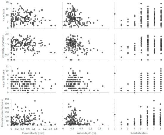
Figure A1.
Hydroecological relationships developed from the spring samples (n = 160) of the benthos-GR dataset between the three abiotic predictors and the four selected biotic response variables-metrics. Substrate classes; 1: Silt, 2: Sand, 3: Fine gravel, 4: Medium gravel, 5: Large gravel, 6: Small stones, 7: Large stones, 8: Boulders. EPT: Ephemeroptera, Plecoptera, Trichoptera.
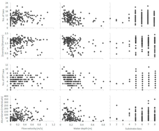
Figure A2.
Hydroecological relationships developed from the summer samples (n = 160) of the benthos-GR dataset between the three abiotic predictors and the four selected biotic response variables-metrics. Substrate classes; 1: Silt, 2: Sand, 3: Fine gravel, 4: Medium gravel, 5: Large gravel, 6: Small stones, 7: Large stones, 8: Boulders. EPT: Ephemeroptera, Plecoptera, Trichoptera.
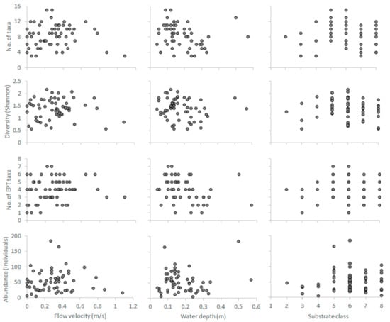
Figure A3.
Hydroecological relationships developed from the autumn samples (n = 60) of the benthos-GR dataset between the three abiotic predictors and the four selected biotic response variables-metrics. Substrate classes; 1: Silt, 2: Sand, 3: Fine gravel, 4: Medium gravel, 5: Large gravel, 6: Small stones, 7: Large stones, 8: Boulders. EPT: Ephemeroptera, Plecoptera, Trichoptera.
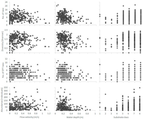
Figure A4.
Hydroecological relationships developed from the RM4-type samples (n = 280) of the benthos-GR dataset between the three abiotic predictors and the four selected biotic response variables-metrics. Substrate classes; 1: Silt, 2: Sand, 3: Fine gravel, 4: Medium gravel, 5: Large gravel, 6: Small stones, 7: Large stones, 8: Boulders. EPT: Ephemeroptera, Plecoptera, Trichoptera.
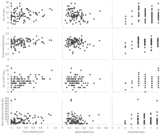
Figure A5.
Hydroecological relationships developed from the RM1-2-type samples (n = 100) of the benthos-GR dataset between the three abiotic predictors and the four selected biotic response variables-metrics. Substrate classes; 1: Silt, 2: Sand, 3: Fine gravel, 4: Medium gravel, 5: Large gravel, 6: Small stones, 7: Large stones, 8: Boulders. EPT: Ephemeroptera, Plecoptera, Trichoptera.
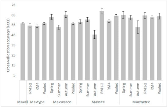
Figure A6.
Mean (gray shaded columns) and standard deviation values from the 10-fold cross validation process for each κ-normalization alternative (model) applied for the Parapeiros reach. CCI: Correctly Classified Instances.
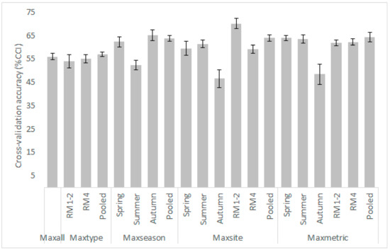
Figure A7.
Mean (gray shaded columns) and standard deviation values from the 10-fold cross validation process for each κ-normalization alternative (model) applied for the Oinoi reach. CCI: Correctly Classified Instances.
References
- Glozier, N.E.; Culp, J.M.; Scrimgeour, G.J. Transferability of habitat suitability curves for a benthic Minnow, Rhinichthys cataractae. J. Freshw. Ecol. 1997, 12, 379–393. [Google Scholar] [CrossRef]
- Lamouroux, N.; Mérigoux, S.; Dolédec, S.; Snelder, T.H. Transferability of hydraulic preference models for aquatic macroinvertebrates. River Res. Appl. 2013, 29, 933–937. [Google Scholar] [CrossRef]
- Gore, J.A.; Layzer, J.B.; Mead, J. Macroinvertebrate instream flow studies after 20 years: A role in stream management and restoration. Regul. River 2001, 17, 527–542. [Google Scholar] [CrossRef]
- Shearer, K.A.; Hayes, J.W.; Jowett, I.G.; Olsen, D.A. Habitat suitability curves for benthic macroinvertebrates from a small New Zealand river. N. Z. J. Mar. Freshw. Res. 2015, 49, 178–191. [Google Scholar] [CrossRef]
- Everaert, G.; Neve, J.D.; Boets, P.; Dominguez-Granda, L.; Mereta, S.T.; Ambelu, A.; Hoang, T.H.; Goethals, P.L.M.; Thas, O. Comparison of the abiotic preferences of macroinvertebrates in tropical river basins. PLoS ONE 2014, 9, e108898. [Google Scholar] [CrossRef] [PubMed]
- Booker, D.J. Generalized models of riverine fish habitat. J. Ecohydraulics 2016, 1, 31–49. [Google Scholar] [CrossRef]
- Vismara, R.; Azzellino, A.; Bosi, R.; Crosa, A.; Gentili, G. Habitat suitability curves for brown trout (Salmo trutta fario L.) in the river Adda, Northern Italy: Comparing univariate and multivariate approaches. Regul. River 2001, 17, 37–50. [Google Scholar] [CrossRef]
- Nykanen, M.; Huusko, A.; Lathi, M. Changes in movement, range and habitat preferences of adult grayling from late summer to early winter. J. Fish Biol. 2004, 64, 1386–1398. [Google Scholar] [CrossRef]
- Maki-Petäys, A.; Muotka, T.; Huusko, A.; Tikkanen, P.; Kreivi, P. Seasonal changes in habitat use and preference by juvenile brown trout, Salmo trutta, in a northern boreal river. Can. J. Fish. Aquat. Sci. 1997, 54, 520–530. [Google Scholar] [CrossRef]
- Studdert, E.W.; Johnson, J.H. Seasonal variation in habitat use of juvenile steelhead in a tributary of Lake Ontario. Northeast. Nat. 2015, 22, 717–729. [Google Scholar] [CrossRef]
- Mérigoux, S.; Dolédec, S. Hydraulic requirements of stream communities: A case study on invertebrates. Freshw. Biol. 2004, 49, 600–613. [Google Scholar] [CrossRef]
- Greenberg, L.; Svendsen, P.; Harby, A. Availability of microhabitats and their use by brown trout (Salmo trutta) and grayling (Thymallus thymallus) in the river Vojman, Sweden. Regul. River 1996, 12, 287–303. [Google Scholar] [CrossRef]
- Heggenes, J.; Saltveit, S.J. Seasonal and spatial microhabitat selection and segregation in young Atlantic salmon, Salmo salar L., and brown trout, Salmo trutta L., in a Norwegian river. J. Fish Biol. 1990, 36, 707–720. [Google Scholar] [CrossRef]
- Kelly, D.J.; Hayes, J.W.; Allen, C.; West, D.; Hudson, H. Evaluating habitat suitability curves for predicting variation in macroinvertebrate biomass with weighted usable area in braided rivers in New Zealand. N. Z. J. Mar. Freshw. Res. 2015, 49, 398–418. [Google Scholar] [CrossRef]
- Jowett, I.G.; Richardson, J.; Biggs, B.J.F.; Hickey, C.W.; Quinn, J.M. Microhabitat preferences of benthic macroinvertebrates and the development of generalized Deleatidium spp. habitat suitability curves, applied to four New Zealand rivers. N. Z. J. Mar. Freshw. Res. 1991, 25, 187–199. [Google Scholar] [CrossRef]
- Bovee, K.D. A Guide to Stream Habitat Analysis Using the Instream Flow Incremental Methodology; Instream Flow Information Paper #12 FWS/OBS-82/26; USDI Fish and Wildlife Service: Washington, DC, USA, 1982; p. 248.
- Li, F.; Cai, Q.; Fu, X.; Liu, J. Construction of habitat suitability models (HSMs) for benthic macroinvertebrate and their applications to instream environmental flows: A case study in Xiangxi River of Three Gorges Reservoir region, China. Prog. Nat. Sci. 2009, 19, 359–367. [Google Scholar] [CrossRef]
- Theodoropoulos, C.; Vourka, A.; Skoulikidis, N.; Rutschmann, P.; Stamou, A. Evaluating the performance of habitat models for predicting the environmental flow requirements of benthic macroinvertebrates. J. Ecohydraulics 2018. [Google Scholar] [CrossRef]
- Van Broekhoven, E.; Adriaenssens, V.; De Baets, B.; Verdonschot, P.F.M. Fuzzy rule-based macroinvertebrate habitat suitability models for running waters. Ecol. Model. 2006, 198, 71–84. [Google Scholar] [CrossRef]
- Vezza, P.; Muñoz-Mas, R.; Martínez-Capel, F.; Mouton, A. Random forests to evaluate biotic interactions in fish distribution models. Environ. Model. Softw. 2015, 67, 173–183. [Google Scholar] [CrossRef]
- Papadaki, C.; Bellos, V.; Ntoanidis, L.; Dimitriou, E. Comparison of West Balkan adult trout habitat predictions using a Pseudo-2D and a 2D hydrodynamic model. Hydrol. Res. 2016, 48, 1697–1709. [Google Scholar] [CrossRef]
- Koutrakis, E.T.; Triantafillidis, S.; Sapounidis, A.S.; Vezza, P.; Kamidis, N.; Sylaios, G.; Comoglio, C. Evaluation of ecological flows in highly regulated rivers using the mesohabitat approach: A case study on the Nestos River, N. Greece. Ecohydrol. Hydrobiol. 2018. [Google Scholar] [CrossRef]
- Theodoropoulos, C.; Skoulikidis, N.; Rutschmann, P.; Stamou, A. Ecosystem-based environmental flow assessment in a Greek regulated river with the use of 2D hydrodynamic habitat modelling. River Res. Appl. 2018, 34, 538–547. [Google Scholar] [CrossRef]
- Kang, H.; Choi, B. Dominant fish and macroinvertebrate response to flow changes of the Geum River in Korea. Water 2018, 10, 942. [Google Scholar] [CrossRef]
- Mouton, A.M.; De Baets, B.; Goethals, P.L.M. Knowledge-based versus data-driven fuzzy habitat suitability models for river management. Environ. Model. Softw. 2009, 24, 982–993. [Google Scholar] [CrossRef]
- Horta, F.; Santos, H.; Tavares, L.; Antunes, M.; Pinheiro, P.; Callisto, M. Assessment of benthic macroinvertebrate habitat suitability in a tropical watershed. In Proceedings of the 7th International Symposium on Ecohydraulics, Concepcion, Chile, 12–16 January 2009; pp. 1–10. [Google Scholar]
- Dakou, E.; D’heygere, T.; Dedecker, A.P.; Goethals, P.L.M.; Lazaridou-Dimitriadou, M.; De Pauw, N. Decision tree models for prediction of macroinvertebrate taxa in the river Axios (Northern Greece). Aquat. Ecol. 2007, 41, 399–411. [Google Scholar] [CrossRef]
- Barry, S.; Elith, J. Error and uncertainty in habitat models. J. Appl. Ecol. 2006, 43, 413–423. [Google Scholar] [CrossRef]
- Conallin, J.; Boegh, E.; Jensen, J.K. Instream physical habitat modelling types: An analysis as stream hydromorphological modelling tools for EU water resource managers. Int. J. River Basin Manag. 2010, 8, 93–107. [Google Scholar] [CrossRef]
- Guisan, A.; Zimmermann, N.E. Predictive habitat distribution models in ecology. Ecol. Model. 2000, 135, 147–186. [Google Scholar] [CrossRef]
- Van de Bund, W. Water Framework Directive Intercalibration Technical Report Part 1, Rivers; JRC Scientific and Technical Reports; Office for Official Publications of the European Communities: Luxemburg, 2009. [Google Scholar]
- Englund, G.; Malmqvist, B. Effects of flow regulation, habitat area and isolation on the macroinvertebrate fauna of rapids in North Swedish Rivers. Regul. River 1996, 12, 433–445. [Google Scholar] [CrossRef]
- Holmquist, J.G.; Schmidt-Gengenbach, J.; Roche, J.W. Stream macroinvertebrates and habitat below and above two wilderness fords used by mules, horses, and hikers in Yosemite National Park. West. N. Am. Nat. 2015, 75, 311–324. [Google Scholar] [CrossRef]
- Monk, W.A.; Wood, P.J.; Hannah, D.M.; Wilson, D.A.; Extence, C.A.; Chadd, R.P. Flow variability and macroinvertebrate community response within riverine systems. River Res. Appl. 2006, 22, 595–615. [Google Scholar] [CrossRef]
- Waddle, T.J.; Holmquist, J.G. Macroinvertebrate response to flow changes in a subalpine stream: Predictions from two-dimensional hydrodynamic models. River Res. Appl. 2011, 29, 366–379. [Google Scholar] [CrossRef]
- Buffagni, A.; Erba, S.; Cazzola, M.; Murray-Bligh, J.; Soszka, H.; Genoni, P. The STAR common metrics approach to the WFD intercalibration process: Full application for small, lowland rivers in three European countries. Hydrobiologia 2006, 566, 379. [Google Scholar] [CrossRef]
- Raleigh, R.F.; Zuckermann, L.D.; Nelson, P.C. Habitat Suitability Index Models and Instream Flow Suitability Curves: Brown Trout; Biological Report 82 (10.124); U.S. Department of Interior, Fish and Wildlife Service, National Ecology Center: Washington, DC, USA, 1986; pp. 57–65.
- Bockelmann, B.N.; Fenrich, E.K.; Lin, B.; Falconer, R.A. Development of an ecohydraulics model for stream and river restoration. Ecol. Eng. 2004, 22, 227–235. [Google Scholar] [CrossRef]
- Leitner, P.; Hauer, C.; Graf, W. Habitat use and tolerance levels of macroinvertebrates concerning hydraulic stress in hydropeaking rivers—A case study at the Ziller River in Austria. Sci. Total Environ. 2017, 575, 112–118. [Google Scholar] [CrossRef] [PubMed]
- Brookes, C.J.; Kumar, V.; Lane, S.N. A comparison of Fuzzy, Bayesian and Weighted Average formulations of an in-stream habitat suitability model. In Proceedings of the International Congress on Environmental Modelling and Software, Ottawa, ON, Canada, 5–8 July 2010. [Google Scholar]
- Theodoropoulos, C.; Skoulikidis, N.; Stamou, A. HABFUZZ: A tool to calculate the instream hydraulic habitat suitability using fuzzy logic and fuzzy Bayesian inference. J. Open Source Softw. 2016, 1, 82. [Google Scholar] [CrossRef]
- Kohavi, R. A study of cross-validation and bootstrap for accuracy estimation and model selection. In Proceedings of the 14th International Joint Conference on Artificial Intelligence, Montreal, QC, Canada, 20–25 August 1995; pp. 1137–1143. [Google Scholar]
- Canadian Hydraulics Centre (CHC). Blue Kenue Reference Manual; Canadian Hydraulics Centre, National Research Council: Ottawa, CA, USA, 2011; p. 211.
- Galland, J.C.; Gontal, N.; Hervouet, J.M. TELEMAC: A new numerical model for solving shallow water equations. Adv. Water Resour. 1991, 14, 138–148. [Google Scholar] [CrossRef]
- Chow, V.T. Open Channel Hydraulics; McGraw-Hill: New York, NY, USA, 1959; p. 680. [Google Scholar]
- Theodoropoulos, C.; Georgalas, S.; Mamassis, N.; Stamou, A.; Rutschmann, P.; Skoulikidis, N. Comparing environmental flow scenarios from hydrological methods, legislation guidelines and hydrodynamic habitat models downstream of the Marathon Dam (Attica, Greece). Ecohydrology 2018, e2019. [Google Scholar] [CrossRef]
- European Union Council. Directive 2000/60/EC of the European Parliament and of the Council of 23 October 2000 establishing a framework for Community action in the field of water policy. Off. J. Eur. Commun. 2000, L327, 1–72. [Google Scholar]
- Linke, S.; Bailey, R.C.; Schwindt, J. Temporal variability of stream bioassessments using benthic macroinvertebrates. Freshw. Biol. 1999, 42, 575–584. [Google Scholar] [CrossRef]
- Sporka, F.; Velek, H.; Bulankova, E.; Krno, I.J. Influence of seasonal variation on bioassessment of streams using macroinvertebrates. Hydrobiologia 2006, 566, 543–555. [Google Scholar] [CrossRef]
- Fonnesu, A.; Sabetta, L.; Basset, A. Factors affecting macroinvertebrate distribution in a Mediterranean intermittent stream. J. Freshw. Ecol. 2005, 20, 641–647. [Google Scholar] [CrossRef]
- Linares, M.S.; Faccioli, G.G.; Freitas, L.M. Benthic macroinvertebrate community structure and seasonal variation in a neotropical stream in the state of Alagoas, Brazil. Biota Neotrop. 2013, 13, 50–54. [Google Scholar] [CrossRef]
- Alomía Herrera, I.; Carrera Burneo, P. Environmental flow assessment in Andean rivers of Ecuador, case study: Chanlud and El Labrado dams in the Machángara River. Ecohydrol. Hydrobiol. 2017, 17, 103–112. [Google Scholar] [CrossRef]
- Boulton, A.J.; Lake, P.S. The ecology of two intermittent streams in Victoria, Australia. III. Temporal changes in faunal composition. Freshw. Biol. 1992, 27, 123–138. [Google Scholar] [CrossRef]
- Harvey, R.; Lye, L.; Khan, A.; Paterson, R. The Influence of Air Temperature on Water Temperature and the Concentration of Dissolved Oxygen in Newfoundland Rivers. Can. Water Resour. J. 2011, 36, 171–192. [Google Scholar] [CrossRef]
- Mérigoux, S.; Lamouroux, N.; Olivier, J.M.; Dolédec, S. Invertebrate hydraulic preferences and predicted impacts of changes in discharge in a large river. Freshw. Biol. 2009, 54, 1343–1356. [Google Scholar] [CrossRef]
- Komínková, D.; Caletková, J.; Vitvar, T. Analysis of environmental flow requirements for macroinvertebrates in a creek affected by urban drainage (Prague metropolitan area, Czech Republic). Urban Ecosyst. 2017, 20, 785–797. [Google Scholar] [CrossRef]
- Fujiwara, M.; Takada, T. Environmental Stochasticity. In Encyclopedia of Life Sciences; John Wiley & Sons Ltd.: Chichester, UK, 2009. [Google Scholar]
- Atluri, G.; Karpatne, A.; Kumar, V. Spatio-temporal data mining: A survey of problems and methods. arXiv, 2017; arXiv:1711.04710. [Google Scholar] [CrossRef]
- Mouton, A.; De Baets, B.; Goethals, P. Data-driven fuzzy habitat models: Impact of performance criteria and opportunities for ecohydraulics. In Ecohydraulics: An Integrated Approach, 1st ed.; Maddock, I., Harby, A., Kemp, P., Wood, P., Eds.; John Wiley & Sons: Hoboken, NJ, USA, 2013; pp. 93–107. ISBN 978-0-470-97600-5. [Google Scholar]
- Hernandez, P.A.; Graham, C.H.; Master, L.L.; Albert, D.L. The effect of sample size and species characteristics on performance of different species distribution modeling methods. Ecography 2006, 29, 773–785. [Google Scholar] [CrossRef]
© 2018 by the authors. Licensee MDPI, Basel, Switzerland. This article is an open access article distributed under the terms and conditions of the Creative Commons Attribution (CC BY) license (http://creativecommons.org/licenses/by/4.0/).