Abstract
This research examines the interrelations in a complex hydrogeological system, consisting of a multi-layered coastal aquifer, the sea, and a surface reservoir (fish ponds) and the importance of the specific connection between the aquifer and the sea. The paper combines offshore geophysical surveys (CHIRP) and on land TDEM (Time Domain Electro Magnetic), together with hydrological measurements and numerical simulation. The Quaternary aquifer at the southern Carmel plain is sub-divided into three units, a sandy phreatic unit, and two calcareous sandstone (‘Kurkar’) confined units. The salinity in the different units is affected by their connection with the sea. We show that differences in the seaward extent of its clayey roof, as illustrated in the CHIRP survey, result in a varying extent of seawater intrusion due to pumping from the confined units. FEFLOW simulations indicate that the FSI (Fresh Saline water Interface) reached the coastline just a few years after pumping has begun, where the roof terminates ~100 m from shore, while no seawater intrusion occurred in an area where the roof is continuous farther offshore. This was found to be consistent with borehole observations and TDEM data from our study sites. The water level in the coastal aquifer was generally stable with surprisingly no indication for significant seawater intrusion although the aquifer is extensively pumped very close to shore. This is explained by contribution from the underlying Late Cretaceous aquifer, which increased with the pumping rate, as is also indicated by the numerical simulations.
1. Introduction
The extensive rural and urban development in coastal areas strongly impacts the coastal environment. This partly occurs via subterranean interaction between land and the sea, which involves a bi-directional flow, including seawater intrusion [1,2] and Submarine Groundwater Discharge (SGD, [3,4,5]). The latter may cause deterioration in water quality of the shallow sea, leading to algae blooms [6,7,8,9]. In some coastal areas, there are surface reservoirs (e.g., fish ponds) above the aquifer which can make the hydrogeological conditions more complex. Worldwide aquaculture has been annually increasing by 8.7% over the past 40 years, the fastest-growing food-producing sector [10]. One of the key environmental concerns about aquaculture is water degradation, due to the discharge of effluents with high levels of nutrients and suspended solids into adjacent waters, causing eutrophication, oxygen depletion and siltation [11]. In the study area, it was shown that the phreatic unit beneath the fishponds area has indeed been deteriorating. It is rich in phosphate, ammonium, Total Organic Carbon (TOC) and manganese, and characterized by strong reducing conditions [12].
Seawater intrusion (SI) is also a global concern, exacerbated by increasing demands for freshwater in coastal zones and predisposed to the influences of rising sea levels and changing climates. Open questions still exist, in particular about the transient SI processes and timeframes, and the characterization and prediction of freshwater–saltwater interfaces over regional scales and in highly heterogeneous and dynamic settings [13].
Numerical solutions have become standard tools for analyzing aquatic systems, which involve a bi-directional flow [14]. Two different modeling approaches have been used in the literature to represent the freshwater–saltwater relationship, one of which is sharp interface approximation [15,16,17], while the other includes a transition zone between freshwater and seawater [18,19,20,21]. Numerical solution with the FEFLOW cod is a common tool to study the salt water interface movement [22]. Yet, extensive measurement campaigns are necessary to accurately delineate interfaces and their displacement in response to real-world coastal aquifer stresses, encompassing a range of geological and hydrological settings [13]. Analytical studies of tide-induced groundwater fluctuations in confined coastal aquifers that extend under the sea have been studied in References [23,24,25] and others. Other studies [24,26] suggested a general analytical solution that showed that the tidal fluctuation in an inland borehole decreases with the confined layer roof length under the sea until a certain distance offshore, wherefrom it remains constant due to the loading effect.
The direct discharge of groundwater to the sea was quantitatively studied by several authors [27,28,29]. A common way of assessing the discharge to the sea is the use of numerical simulations and analytical solutions of the water flow regime [30,31]. This is aided by geophysical [32] and the use of chemical and isotopic tracers, including radon and radium isotopes [5,6,33]. Seepage meters, which are deployed on the seabed, provide direct local measurements of fluxes [34].
The objective of this study was to investigate the effect of the marine and terrestrial boundary conditions on the hydraulic connections between the sea and a multi-layered coastal aquifer and its resultant seawater intrusion, using numerical simulations and field observations.
2. Hydrogeological Background of the Study Area
The study area extends from Mt. Carmel to the sea at the southern Carmel coastal plain, Israel (Figure 1). It is covered by Quaternary Nilotic sands with a total thickness of about 40 m, which are underlain by Late Cretaceous carbonate basement [35]. Located on its eastern part are the Taninim springs at +3 m asl, which are the northern discharge of the Late Cretaceous Yarkon–Taninim carbonate Aquifer (Figure 1). These springs are the principal source of water for fishponds in this area. The spring water is brackish (1500–2000 mg L−1 Cl), which is due to the mixing of fresh groundwater with saline water that exists in the western part of the Late Cretaceous aquifer [36]. The Late Cretaceous carbonates change from limestone and dolomite facies in the Mt. Carmel area on its eastern side to a chalky facies on its western (seawards) side [35,37], which prevents the direct flow of groundwater from the Late Cretaceous aquifer to the sea and forces the water to discharge in the Taninim springs through Quaternary sediments (Figure 2). Some of this water flows westward through the Pleistocene sediments and plays an important role in the water balance of the coastal Quaternary Aquifer [12,38,39,40].
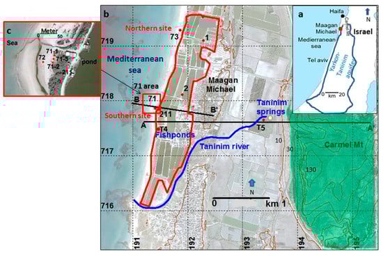
Figure 1.
(a) Location map of the research area. (b) Borehole locations are shown as red points. Ponds’ area is circled by a Red line. The area where the Cretaceous aquifer is exposed is colored green, and the Quaternary coastal aquifer is grey. (c) The left inset is an aerial photo of wells 71 area. The hydrogeological sections presented in Figure 2 and Figure 3a were taken along the lines A–A’ and B–B’.
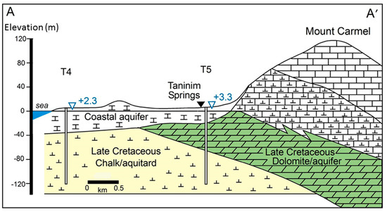
Figure 2.
Hydrogeological section in the research area (A–A’ in Figure 1), modified after [35]. The coastal aquifer overlays Late Cretaceous limestone and dolomite aquifer in the east and chalk aquitard in the west. The dolomite aquifer (green) is the main source to the Taninim springs. The upper units in the Mount Carmel area, consisting of limestone and chalky limestone, are also of Late Cretaceous age. The blue number indicates the pre-utilization heads.
The thickness of the coastal Quaternary aquifer in the study area is 40 m (Figure 3a). It includes three sub-aquifers (Figure 3a). The shallow sub-aquifer is a phreatic Holocene sandy unit (unit A) with a thickness of several meters, which is separated from the underlying Pleistocene calcareous sandstone (locally called Kurkar) aquifer by a clay unit. The Pleistocene Kurkar is subdivided by another clay layer at an approximate depth of 20 m into two confined units, B and C, which in turn are underlain by the Late Cretaceous chalks. The coastal area is characterized by two N–S oriented Kurkar ridges on its western side, with the western one often partly or completely submerged [41,42]. In the study area, fish ponds occupy the area between the eastern ridge and the sea (Figure 1 and Figure 3a), with an annual infiltration to the aquifer of about 9 × 10⁶ m3year−1 [40].
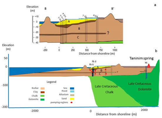
Figure 3.
(a) Detailed hydrogeological section of the coastal aquifer in the study area (B–B’ in Figure 1). The coastal aquifer is subdivided into three units which are separated by clay layers: upper phreatic sandy unit (A) and two confined calcareous sand (Kurkar) units (B and C). (b) A hydrogeological cross section in the southern part of the studied area. The eastern boundary of the model is not shown (4 km from the shoreline).
The confined units B and C, which contain brackish water (1500–2000 mg L−1 Cl), have been extensively exploited since 2005 as raw water for a desalination plant and for the fish ponds. The pumping in this area currently reaches ~20 × 106 m3year−1. Although exploitation is very high, groundwater level in these units is quite stable, and seawater intrusion is very limited [43]. Geochemical mass balance indicates that more than 85% of the water in units B and C derives from the underlying Late Cretaceous aquifer [12], while the ponds contribution is no more than 3 × 10⁶ m3year−1 [12]. This suggests that most of the ponds’ losses flow through unit A to the sea.
3. Field Methods
The relations between the aquifer and the sea were studied in two coastal sites, 1.5 km apart (Figure 1). Groundwater level was mainly studied in boreholes drilled at 45–70 m from the sea to a depth of 10–40 m (wells 71-1, 71-2, 71-3, 72, 73, Figure 1), each opened to a different unit, A, B or C. We also used data from a few observation boreholes located farther inland (1500–600 m from the sea).
TDEM (Time Domain Electro Magnetic) measurements were conducted to locate the fresh–saline water interface. Surveys in coastal aquifers [44,45,46,47] show that this method is feasible for detecting the interface due to the very high resistivity contrast between the sea water saturated portion of the aquifer (1–2 ohm-m) and the fresh water part, which is characterized by values more than 10 ohm-m [45]. The survey was conducted using the Geonics EM-67 TDEM system (GEONICS Ltd., Mississauga, ON, Canada). The TDEM method utilizes a step-wise current flowing in a squared transmitter loop that produces a transient secondary electromagnetic field in the subsurface. Depending on the required exploration depth, the loop size varies between tens by tens meters to hundreds by hundreds meters. In the described survey, the loop size was 25 × 25 m. The electromagnetic field induced into the ground produces a secondary response, which is picked up on the surface by a receiver coil. The data were analyzed using two different inversion methods, smooth inversion, and sharp boundary inversion. The combination of solutions usually improves both the accuracy and reliability of decryption. The TDEM survey was conducted along two E–W traverses, one in the southern site and the second in the northern site (Figure 1). In each profile, three loop measurements were carried out between the shore and approximately 80 m inland. The TDEM survey and the interpretation of the data were conducted by the Geophysical Institute of Israel.
CHIRP sub bottom profiler was used for mapping of the shallow sub-seafloor sediments. The seismic survey was conducted with the “Adva” boat of the IOLR (Israeli Oceanography and Limnology Research), which also carried a Trimble AgGPS 132–receiver, an Odom Echotrack MKIII depth meter, and Oceanographer navigator. The depth meter was calibrated by Bar check and sound wave velocity meter in water, SV-2000 Smart sensor, which belongs to AML company (Hong Kong, China). The velocity of sound waves in the submarine sand and clay was taken as 1700 m/s, while for the sea water, it is 1530 m/s [48]. The CHIRP survey and the interpretation were conducted by Arik Golan from IOLR.
Electric conductivity (EC) profiles were conducted in the monitoring wells 71-1, 71-2, and 71-3 (locations in Figure 1) using a Robertson Geologging (RG) profiler.
Water level was measured by Schlumberger divers with 5 min frequency in wells 1, 2, 71-1-3, and 73. Sea Level was measured at Hadera MedGloss station, 2.5 km from the shore by IOLR (Israeli Oceanography and Limnology Research).
Slug tests were conducted for the determination of the hydrological conductivity in the aquifer. In each well, we conducted five tests, including three nitrogen injections, slug in and slug out. The slug tests were conducted in the monitoring wells 1, 2, 71-1, 71-2, 72, and 71-3. Results are presented in the Supplementary Materials, while the interpretation follows the procedure given in [49].
Point dilution test with Uranine solution was implemented in well 71-3, which penetrates the shallow phreatic aquifer. The tracer, with a concentration of 1000 ppb was injected uniformly along the hole, and time series concentrations were measured by a Fluorometer (Turner Design, San Jose, CA, USA). The rate of decrease in tracer concentration was used to calculate the horizontal groundwater velocity in the well by the procedure described in Reference [50]. Results are given in The Supplementary Materials.
Interference recovery test was conducted by analyzing the level recovery in wells 71-2 (unit B) and 71-1 (unit C) after stopping pumping in the nearby (within 50 m) well 211 (Figure 1). Test results were used to calculate the transmissivity and the storativity of the aquifer, using the solution of Reference [51] for confined aquifers.
Radon (222Rn) was sampled in both seawater and groundwater, using pre-vacuumed 4.5 L glass bottles. Seawater was sampled close to the seafloor in coastal water up to 700 m offshore (maximum water depth of 5 m) and groundwater was sampled from wells (the 71 series) using a peristaltic pump. 222Rn activities were measured by alpha-scintillation Lucas cells, using a modified emanation technique. In this method, helium is circulated and bubbled through the sampling bottle, resulting in the extraction of 222Rn. The radon is trapped on activated charcoal (at −90 °C) and then transferred to the Lucas cell.
Numerical simulations were conducted with the 2D FEFLOW program, which is a finite element code, allowing the examination of both flow and salt transport. To deal with the specific process in a precise way, a very dense net of triangular elements (~100,000) was built (element size range from ~1 m to 10 m). The model configuration included seven layers, in accordance with the geological section of the southern Carmel coastal plain: five layers in the Quaternary section and two in the underlying Late Cretaceous (Figure 3b). The conceptual model and model calibration were based on field measurements, presented and discussed in Section 4, including seabed geology (provided by the CHIRP survey), the TDEM survey, EC profiles, hydrological field experiments, and groundwater levels. The length of the model section is 7 km, from the sea on its west to the Carmel Mountains on its eastern end.
4. Field Results
4.1. Water Level
Figure 4a presents sea level and groundwater levels at the southern (wells 71-1, 71-2, 71-3) and the northern sites (well 73, Figure 1). Groundwater table in the intermediate confined unit (B) at the southern site was 0–0.3 m asl, while in the phreatic unit (A) and the deeper confined unit (C) it was higher, 1.5 and 1.3 m asl, respectively. The level in well 71-2 (unit B) and well 71-1 (unit C) was affected by a nearby pumping well, which is reflected in level increase during pumping breaks (i.e., return to more natural conditions) by 80 and 20 cm, respectively. At the northern site, water level in Unit B was higher (~1 m asl). In Figure 4b, we compare sea level and groundwater levels by zeroing to their mean values. Tidal fluctuation was hardly observed in the phreatic unit (southern site) at 70 m from the sea (1 cm), while it was clearly evident in the confined units B and C (amplitudes of up to 13 and 9 cm, respectively, during spring tide, compared with 21 cm at the sea, Table 1). At the northern site, maximum amplitude in unit B at 70 m from the sea and during the same period was just 7 cm. Level fluctuation decreased with distance from shore (4.5 and 3 cm at 300 m and 500 m, respectively, at the 2 and 1 sites, Table 1).
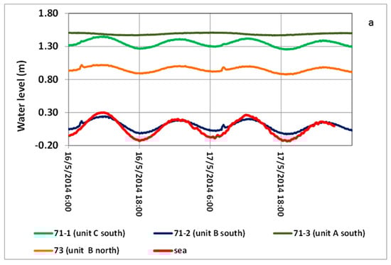
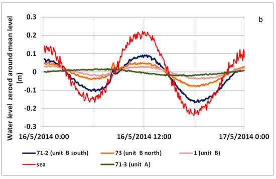
Figure 4.
Detailed (5 min) water level time series in monitoring wells and the sea. (a) a 48 h level fluctuations; (b) 24 h superimposed levels of different wells and the sea, zeroed around their mean level. See well locations in Figure 1.

Table 1.
Maximum tidal amplitudes in different units and distance from shoreline during May 2014.
4.2. EC Profiles
Electrical conductivity profiles in units C, B, and A, at 70 m from shore, are presented in Figure 5. Units A and C show low and uniform EC values (5–6 mS/cm, similar to the natural salinity in this area) while unit B shows an interface composed of two steps. The EC changes from 5.5 mS/cm at a depth of 12 m to 40 mS/cm at a depth of 24 m.
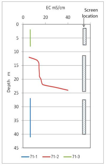
Figure 5.
EC profiles in wells 71-3, 71-2, 71-1 penetrating the three Quaternary units (A, B and C, respectively), 70 m from the sea, at the southern site of Ma’agan Michael.
4.3. Electrical Resistivity—TDEM
The interpreted TDEM results from the southern site are in agreement with the EC borehole profiles. According to the TDEM, there is a large resistivity difference in unit B between the southern and the northern sites (Figure 6 and Figure S1 in the Supplementary Material), whereby relatively fresh groundwater is found in the northern site (resistivity of about 10 ohm-m), while brackish groundwater is exhibited in the southern site (resistivity of 3–5 ohm-m). The TDEM results also suggest that relatively fresh water occurs in unit C at both sites (Figure 6 and Figure S1 in the Supplementary Material).
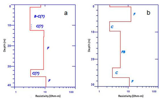
Figure 6.
Representative TDEM (Time Domain Electro Magnetic) profiles at the northern site (a) and at the southern site (b). In the north, high resistivity is observed for both unit B and C (10 Ohm-m), while in the south the middle aquifer (unit B) has low resistivity (5 Ohm-m). The letters along the profile are the interpretation of the resistivity values: F—Fresh, B—Brackish, FB—fresh–brackish, C—Clay unit. Additional TDEM profiles are included in Figure S1 in the Supplementary Material.
4.4. Seismic Reflection
A CHIRP survey was conducted along eight parallel E–W offshore transects, 2 km each (Figure 7). The interpretations of the seismic data allowed the identification of the top of the upper clay and of the intermediate Kurkar unit (B). CHIRP results also show areas, where the clay layer is missing and the Kurkar rock is exposed at the seabed (e.g., Figure 7). The results of the survey suggest that there is a major difference between the southern and the northern sites with regards to the continuation of the upper clay layer (Figure 8). While at the southern site the clay was eroded around 100 m from shore line, at the northern site the clay layer is mostly continuous, and if missing, it occurs in limited areas relatively far from shore (>700 m). A sketch of the geological section, which expresses the difference between the southern and the northern site, is presented in Figure 9. The CHIRP survey also identified a “hot spots” (weak acoustic reflection in the high frequently CHIRP channel) along Section 2 and Section 3, which was interpreted as groundwater discharge at one of the unit B exposure sites (Figure S8 in the Supplementary Material).
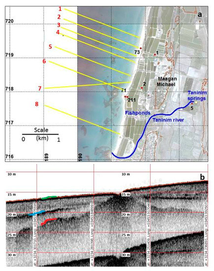
Figure 7.
Location map of the CHIRP survey lines (a) and CHIRP seismic interpretation along part of Section 2 (b). The top calcareous sandstone (‘Kurkar’) layer is shown by red line, the top clay layer by blue line and the seabed by green line.
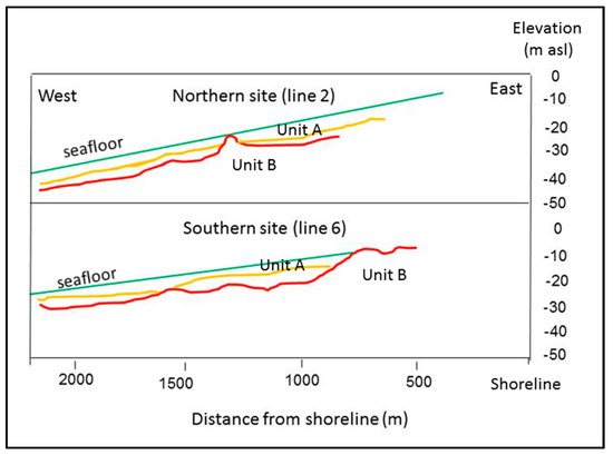
Figure 8.
Interpretation of CHIRP lines 6 and 2 (location in Figure 8). The top Kurkar layer is shown by red line, the top clay layer by orange line and the seabed by green line.
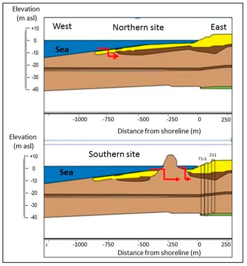
Figure 9.
Schematic geological section in the northern and southern sites. In the southern site, the clay is eroded near the shore (100 m), therefore, the Kurkar unit is in direct contact with the sea closer to shore.
4.5. Radon
The average Radon activity in water sampled onshore from the confined Kurkar units B and C (wells 71-2 and 71-1, Table 2) was 735 dpm/L, quite similar to the findings at Dor Bay, 5 km to the north [5]. Most seawater samples (10–800 m from shore, all taken close to seabed) had much lower activities (0–2 dpm/L). One exception of 10.9 dpm/L was found at 5 m depth, above a seabed Kurkar exposure, about 700 m offshore at the northern site (Figure S9 in the Supplementary Material).
Table 2.
Radon activity in groundwater and fish pond water (dpm/L) from Aug 2010 and May 2011.
4.6. Hydrological Tests
Table 3 summarizes the hydraulic parameters, obtained from the field experiments, which are later used as the initial hydraulic parameter for the model calibration (Section 5). The slug and the interference recovery tests yielded similar hydraulic conductivity values, 45 and 68 m/day in unit B and 66 and 109 m/day in unit C, respectively. Since the slug is a local test, which is influenced by the well structure, we prefer to use the values obtained from the interference test, whenever available. The detailed results of the field experiments are given in Figures S2–S7 and Tables S1–S3 in the Supplementary Material.
Table 3.
Hydraulic Transmissivity, conductivity, and Storativity, determined by field tests (slug, point dilution, and the interference recovery tests).
Point dilution results from well 71-3 suggest that flow rate (v) in unit A was 5.9 m/day. Considering the hydraulic gradient near the shore (j = 1.5 m/70 m), and assuming porosity (n) of 0.15 for the sandy matrix, the hydraulic conductivity for the phreatic sand unit is 42 m/day (k = nv/j). This value is somewhat higher than the value of 13.2 m/day obtained from the slug test conducted in the same well. For the model calibration, we choose an intermediate value of 30 m/day.
5. Numerical Modeling
5.1. Geological Configuration
The eastern boundary was set at ~2 km east of the Taninim springs, where Late Cretaceous dolomite rocks are exposed at the foot of Mt. Carmel. This allowed the examination of the effect of pumping from the coastal Quaternary aquifer on the Late Cretaceous aquifer. The western boundary was set 3 km offshore, based on the CHIRP results, which showed that the onshore hydrogeological configuration continues beneath the seabed. Based on the offshore differences between the northern and the southern sites (see CHIRP results above), we conducted simulations with two different hydrogeological configurations. In the first, the upper clay unit extended 800 m offshore, while in the second, simulating the southern site, it reached just 100 m offshore (Figure 9).
5.2. Hydraulic Properties
The hydraulic conductivity of the Late Cretaceous dolomites was assumed to be 200 m/day [52], while for the Late Cretaceous chalks, underlying the Quaternary aquifer, a value of 1 m/day was assigned. Hydraulic parameters in the coastal aquifer were estimated according to the pumping results and the slug tests, conducted during this study (Table 2). After calibration, the hydraulic conductivity was taken to be somewhat higher than field estimates, 100 and 160 m/day for units B and C, compared with 66 and 100 m/day, respectively. On the eastern part, where no division to sub-aquifers was observed, a value of 100 m/day was assumed for the whole Quaternary aquifer. Conductivity of the phreatic sand unit (A) was assumed 30 m/day (between the 42 m/day of the point dilution results and 13 m/day of the slug test). The specific storage was assumed 10−4 m−1 for both units, porosity was taken as 0.1, and dispersion as 5 m/day, with anisotropy of 10:1 (longitudinal to transversal ratio).
5.3. Boundary and Initial Conditions
We used two extreme scenarios for water level at the eastern boundary: level of +5 m, as was used to be in the more pristine conditions [37], and level of +3 m, as is the current case due to over-pumping from the Late Cretaceous Yarkon–Taninim carbonate Aquifer. The head at each offshore point was calculated as water depth multiplied by the seawater density. The salinity at the western boundary was taken as 39,000 mg/L TDS (Total Dissolved Solutes) and the specific gravity was 1.027, similar to that of the coastal Mediterranean Sea. Based on estimates of the Hydrological Survey of Israel, we used infiltration coefficient of 35% (average of 200 mm/year) for the western 0.7 km of the coastal plain, which is covered by sand and some clay, while a coefficient of 18% was assumed for the clayey soils of the eastern part. Total ponds losses were assumed as infiltration of 13 mm/day (about 3 m3year−1 for 1 km of coast), following [40].
The simulation was performed with the above conditions until steady state was reached. These steady-state conditions were used as initial conditions for the transient modeling after pumping began.
5.4. Pumping Regime
Withdrawal from the coastal aquifer in the studied area during 2005–2015 was 18–20 m3year−1. According to chemical balances [12], the fish ponds’ contribution to the Kurkar aquifer (units B) is 2–3 × 10⁶ m3year−1. This value was subtracted from the total pumping instead of adding artificial recharge from the pond, and, thus, the effective pumping was assumed ~15 × 106 m3year−1. Since the length of the coast in the studied area is about 3 km, the pumping in the model was taken as 5 × 10⁶ m3year−1 per 1 km coast. Most pumping wells are perforated along the whole Pleistocene section and pump from both confined units (B and C). Therefore, the model assumes that of the existing four pumping wells, two pump from unit B and the other two from unit C (Figure 3b, red points).
5.5. Calibration of the Model
The calibration was done by comparing the dynamic results of the simulation to field measurements of water level and salinity in the different aquifer units at the southern site, near the sea. This includes: (1) water level in units C and B (1.3 and 0.3 m, respectively); (2) water salinity in unit B at the site (occurrence of FSI), and (3) low salinity in unit C. Because the pristine level conditions in the different units are not known, we calibrated the model only for the dynamic condition (pumping of 5 × 10⁶ m3year−1 per 1 km coast). The simulation was conducted for the maximum and minimum heads at the eastern boundary (+5 and +3 m). Both scenarios were simulated until the flow field stabilized.
6. Simulation Results
6.1. Seawater Intrusion
The fresh–saline water interface in unit B is located where the confining clay layers breach the seabed, which is further off-shore at the northern site than in the southern site (Figure 10a,b). The location of the interface does not change much after pumping in the case of an eastern boundary head of +5 m (not shown in Figure 10), while in the case of +3 m head, pumping results in significant inland shift of the interface in unit B (Figure 10c). The location of the interface after 1000 days of pumping is shown in Figure 10c,d, and the change in salinity in unit B at a distance of 70 m from the shore (in observation point 2, Figure 10) is shown in Figure 11. This shift occurs both at the southern and at the northern site, but while at the southern site the interface reached the pumping wells, no salinization occurred at the northern site during the first few years (Figure 11). At both sites, penetration of seawater in unit C was very limited.
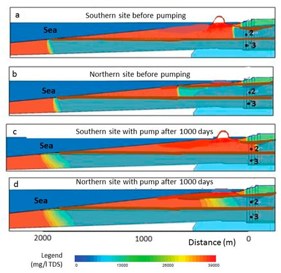
Figure 10.
The location of the fresh–saline water interfaces in the different sub-aquifers: before pumping in the southern site (a); and in the northern site (b); after 1000 days of pumping with eastern boundary water level of +3 m, in the southern site (c) and the northern site (d). “2” and “3” denote units B and C.
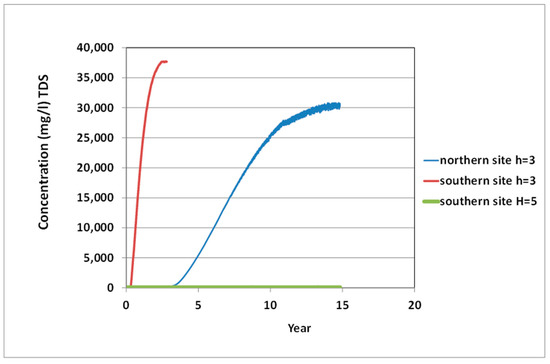
Figure 11.
The simulated salinity in unit B at a distance of 70 m from the shore in the northern and southern sites (point 2 in Figure 10), for different boundary conditions (level of +5 and +3 m at the eastern model border).
6.2. Water Balance and Levels in Units B and C
The calculated water levels in observation boreholes at the pristine state and after pumping are given in Table 4. To maintain the average water level of +1.3 m in unit C at 70 m from shore (as observed in the field, Figure 4a), a significant amount of water must enter from the base of the coastal aquifer, namely from the Late Cretaceous aquifer. According to the results of the model, the increase in pumping from the coastal aquifer causes a ~0.4 m decrease in Late Cretaceous water level around the Taninim springs (borehole 5, Figure 1). The calculated water volumes entering from the Late Cretaceous aquifer to the coastal aquifer are shown in Table 5. In the natural state, when the water level in the eastern boundary was ~+5 m, this flux is estimated at 2.2 × 10⁶ m3year−1 per 1 km of coast, which is almost the natural flow to the sea. After the initiation of pumping from the coastal aquifer (5 × 10⁶ m3year−1 per 1 km coast), flux from the east increased to 5.4 × 10⁶ m3year−1 per 1 km, and the discharge to the sea from units B and C almost ceased (Table 6). With an eastern boundary water level of +3 m (over-exploitation of the Late Cretaceous Yarkon–Taninim aquifer), the pristine water flow into the coastal aquifer was smaller (1.7 × 10⁶ m3year−1 per 1 km coast), and after pumping commenced, flux from the east increased to 4.6 m3year−1 per 1 km (Table 5). Under these conditions, discharge from the confined units to the sea is negative (unit B: −0.7 and unit C: −0.2 × 10⁶ m3year−1, Table 6), and seawater intrudes as to keep the water balance in these units.
Table 4.
Simulation-calculated water levels in observation boreholes, before and after pumping in the southern and northern sites under different boundary conditions. The measured levels in wells 71-1, 71-2, which represent the level after pumping, are presented in Figure 4a.
Table 5.
Calculated water input from the Late Cretaceous aquifer to the coastal aquifer in the pristine case and after pumping of 5 × 10⁶ m3year−1 per 1 km coast from the coastal aquifer, with eastern boundary level of +5 m and + 3 m.
Table 6.
Calculated flux to the sea with and without pumping from the coastal aquifer. In brackets, is the flux from unit A affected by ponds losses. The natural discharge to the sea is about 2.2 m3year−1 per 1 km.
6.3. Flow in Unit A
The model results show that the estimated losses of 3 × 10⁶ m3year−1 per 1 km coast from the ponds are divided between infiltration into unit A, which then flows directly to the sea, and unit B (about 1.8 and 1.2 × 10⁶ m3year−1, respectively). The simulated water level in unit A varies between 5.5 m upstream and 1.5–2 m near the coast, which fits the measured levels (+5.5 m in well 2a and +1.5 m in well 71-3, 300 and 70 m from the coast, respectively, Figure 1 and Figure 4a). The estimated flux from unit A between well 71-3 and the sea, using Darcy equation (J = 1.5 m/70 m, T = 195 m2/day, Table 3) is 1.5 × 10⁶ m3year−1 per 1 km coast.
6.4. Tidal Effects
The difference in sub-sea extension of the confined layer B between the southern and northern site results in different tidal amplitudes and water level in the observation wells 70 m on shore. The simulations suggest larger tidal amplitudes and lower level in unit B at the southern site, compared with the northern one (Figure 12), in agreement with our observations (wells 71-2 and 73, Table 1, Figure 12).
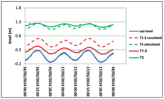
Figure 12.
Measured and calculated water levels in observation wells in unit B, located 70 m from shore in the northern site (well 73) and in the southern site (well 71-2).
7. Discussion
7.1. Offshore Extension of the Confining Layer and Seawater Intrusion
The above simulations, as well as field results, highlight the importance of the boundary hydrological conditions on seawater intrusion in a multi-layered coastal aquifer. The difference in the seaside boundary conditions is expressed in the numerical simulations in different locations of the interface zone. While the interface at the southern site reaches the shoreline within a few years after pumping began, the interface at the northern site, where the clay layer extends farther seawards, is still located under the sea. These results are consistent with those of the TDEM, which showed relatively fresh groundwater in unit B of the northern site, while a clear interface at the southern site. The simulations and the field results show that the confined clay layer continuity in the sea has an important role in delaying seawater intrusion even when the aquifer is extensively exploited. The difference in the sub-sea extension of the upper confining clay layer also results in a difference in the groundwater tidal amplitudes, which are larger at the southern site (Table 1, Figure 4b), where the clay is missing closer to shore, than at the northern site, where the clay is mostly continuous to at least 700 m from shore. This difference in tidal amplitudes is also reflected in the simulations (Figure 12), although the measured amplitudes at borehole T-73 are somewhat smaller than the simulated ones. This difference could be eliminated by assigning larger storativity to the aquifer. However, this will cause a significant lag in the arrival of a tidal signal in the aquifer, in disagreement with our observations (Figure 13). Alternatively, we suggest that the relatively small amplitudes are due to the leaky nature of the thin confining layer, which would tend to damp the amplitude in the inland aquifer [26]. The numerical model also highlighted the importance of the land side (eastern) boundary condition, in the Late Cretaceous aquifer. Using high boundary heads (natural condition, before pumping started), seawater intrusion does not occur even under high exploitation, while with lower boundary heads, the aquifer is more liable to seawater intrusion.
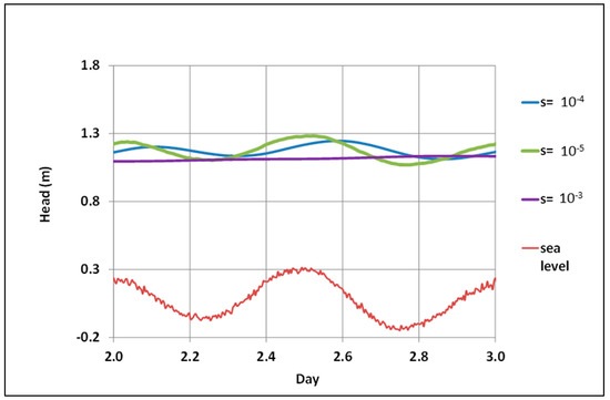
Figure 13.
Transient heads at observation point 2 in the northern site (indicated in Figure 10, representing borehole 73) for various values of storativity/specific staorge of the confined unit B. Using high storativity, the aquifer tidal signal lags significantly after the sea, which is in disagreement with our observations.
7.2. The Impact of Pumping on the Adjacent Aquifer
The numerical model was used to quantify the flow regime into the multi-layered aquifer system. Previous works [12,38,39,40] showed hydrogeological and geochemical evidence for contribution from the Late Cretaceous aquifer to the coastal aquifer, whose extent was not clear. Our modeling examined more quantitively the suggestion that the Late Cretaceous aquifer is the main source of water (about 85%, [12]) to the coastal Quaternary aquifer (units B and C). The results of the simulations support this suggestion and show that increasing exploitation from the coastal aquifer causes an increase in the component of the water arriving from the adjacent Late Cretaceous aquifer. This increase in pumping also affects the discharge of the nearby Taninim springs. The model shows that to maintain the average water level of +1.3 m in the confined unit C at 70 m from shore under pumping conditions, a significant amount of water must enter from the base of the coastal aquifer, namely from the Late Cretaceous aquifer at the foot of Mt. Carmel, where the Quaternary rocks are in hydraulic contact with Late Cretaceous dolomites. This is possible due to the high hydraulic conductivity in both Pleistocene and the Late Cretaceous aquifer (100–200 m/day).
7.3. Discharge to the Sea
According to water budgets, water losses from the fishponds to the aquifer are about 9 × 10⁶ m3year−1 [40]. The connection of the ponds with units B and C is limited due to the existence of a clay layer under the ponds area [12], which limits infiltration to 2–3 × 10⁶ m3year−1. This implies that most pond losses flow through unit A to the sea. The simulation results show that although unit A is of very small thickness (up to 6 m), it transfers 1.8 × 10⁶ m3year−1 per 1 km coast, while keeping the level at +5.5 m and +1.5 m at 300 m and 70 m from the sea, respectively. These are, indeed, also the levels that were measured in the field. Considering fishpond length of 3 km, the flow from unit A to the sea is 5.4 m3year−1. According to simulation results, the flow from units B and C to the sea after the development of pumping from the coastal aquifer is relatively small and changes according to the eastern boundary condition between almost zero to negative values.
Radon activity in the calcareous sandstone (Kurkar) units was around 450 dpm/L, similar to the activities measured in groundwater from Dor bay, ca. 5 km to the north, where Reference [5] showed that the SGD radon source is the fresh groundwater and used it to calculate the fresh water discharge to the bay. Areas where the confided clay layer is eroded and the Kurkar is exposed on the seabed are suitable for Submarine Groundwater Discharge. Indeed, a radon hot spot (10.9 dpm/L) was found 500 m offshore at the northern site, where SGD was inferred also by the CHIRP results. Based on the radon–salinity mixing line between seawater and the Kurkar water source, the seawater at this point contains at least 2.5% freshwater derived from the Kurkar unit.
Since groundwater in unit A is highly polluted in several places [12], the effect of this SGD on the quality of the shallow sea could be significant.
8. Summary and Conclusions
This research combines field measurement and numerical simulation to examine the interrelations between a multi-layered coastal aquifer, a surface reservoir (fish ponds) and the sea. The measurement includes offshore geophysical surveys (CHIRP) and on land TDEM, together with hydrological tests and water level measurements. The main conclusions of this research are:
- (1)
- The location of the hydraulic connection between a confined sub-aquifer and the sea (the distance from the shoreline) is shown to be a very important factor in the determination of the extent of seawater intrusion.
- (2)
- The location of the aquifer-sea connection also affects the tidal fluctuations in the monitoring boreholes.
- (3)
- Submarine CHIRP mapping indicates that the continuity of the confining clay varies on short spatial scales (2 km).
- (4)
- In the Numerical model, this difference in clay continuity resulted in different extent of seawater intrusion in the shallow confined layer.
- (5)
- Numerical simulations indicate that water level, as well as seawater intrusion in coastal aquifers, could be highly affected by its connection with an underlying aquifer.
We show that the exact location of the connection between the confined aquifer unit and the sea plays a significant role on the sensitivity of an aquifer unit to seawater intrusion. These geophysical methods need to be used to determine this location in the different part of the coastal aquifer when deciding on the exact pumping regime of the aquifer. Another practical way to estimate this location is by the tidal amplitude in an observation well near the seashore. We, therefore, suggest that these methods be used as managerial tools in the vicinity of the sea to avoid large seawater intrusion.
Supplementary Materials
Supplementary Materials are available online at http://www.mdpi.com/2073-4441/10/10/1426/s1.
Author Contributions
A.T. did the field work, conduct the modeling and wrote the manuscript, Y.W. took part in writing and in the field study, S.W. was responsible for the simulations, M.G. did the TDEM study and Y.Y. took part in the modeling and the writing of the paper.
Funding
This project was partly funded by a Water Authority of Israel grant 4500445470 and by a USAID MERC grant M29-073.
Acknowledgments
We are grateful to people from the Geological Survey of Israel for their support: to Halel Lutzki for the field tests, to Iyad Swaed for his help with the new wells, to Haim Hemo for the EC profiles, to Nili Almog and Bat-Sheva Cohem for their help in drawing the figures. Thanks to Yehuda Shalem and the Radon laboratory team in the HU for the help in the Radon sampling and analyzing. We are grateful to Eldad Levi from the Geophysical Institute for the support in the TDEM survey and to Aric Golan from the IOLR to the support with the CHIRP survey and the seismic interpretation. Thanks to Einat Magal for the help with the “Point dilution test” and to Yossi Berchman from Maagan Michael for their cooperation.
Conflicts of Interest
The authors declare no conflicts of interest.
References
- Bear, J.; Cheng, A.H.D.; Sorek, S.; Ouazar, D.; Herrera, I. (Eds.) Seawater Intrusion in Coastal Aquifers: Concepts, Methods, and Practices; Kluwer Academic Publishers: Dordrecht, The Netherlands; Boston, MA, USA; London, UK, 1999. [Google Scholar]
- Post, V. Fresh and saline groundwater interaction in coastal aquifers: Is our technology ready for the problems ahead? Hydrogeol. J. 2005, 13, 120–123. [Google Scholar] [CrossRef]
- Winter, T.C. Numerical simulation of steady state three-dimensional groundwater flow. Water Resour. Res. 1978, 14, 245–254. [Google Scholar] [CrossRef]
- Moore, W.S. Large groundwater inputs to coastal waters revealed by 226Ra enrichments. Nature 1996, 380, 612–614. [Google Scholar] [CrossRef]
- Weinstein, Y.; Burnett, W.C.; Swarzenski, P.W.; Shalem, Y.; Yechieli, Y.; Herut, B. The role of coastal aquifer heterogeneity in determining fresh groundwater discharge and seawater recycling: An example from the Carmel coast, Israel. J. Geophys. Res. 2007, 112, C12016. [Google Scholar] [CrossRef]
- Moore, W.S. The subterranean estuary: A reaction zone of ground water and sea water. Mar. Chem. 1999, 65, 111–125. [Google Scholar] [CrossRef]
- Woessner, W.W. Stream and fluvial plain ground water interactions: Rescaling hydrogeologic thought. Ground Water 2000, 38, 423–429. [Google Scholar] [CrossRef]
- Linderfelt, W.R.; Turner, J.V. Interaction between shallow groundwater, saline surface water and nutrient discharge in a seasonal estuary: The Swan–Canning system. Hydrol. Process. 2001, 15, 2631–2653. [Google Scholar] [CrossRef]
- Trefry, M.G.; Svensson, T.J.A.; Davis, G.B. Hypoaigic influences on groundwater flux to a seasonally saline river. J. Hydrol. 2007, 335, 330–353. [Google Scholar] [CrossRef]
- Herbeck, S.L.; Unger, D.; Wu, Y.; Jennerjahn, C.T. Effluent, nutrient and organic matter export from shrimp and fish ponds causing eutrophication in coastal and back-reef waters of NE Hainan, tropical China. Cont. Shelf Res. 2013, 57, 92–104. [Google Scholar] [CrossRef]
- Burford, M.A.; Costanzo, S.D.; Dennison, W.C.; Jackson, C.J.; Jones, A.B.; McKinnon, A.D.; Preston, N.P.; Trott, L.A. A synthesis of dominant ecological processes in intensive shrimp ponds and adjacent coastal environments in NE Australia. Mar. Pollut. Bull. 2003, 46, 1456–1469. [Google Scholar] [CrossRef]
- Tal, A.; Weinstein, Y.; Yechieli, Y.; Borisover, M. The influence of fish ponds and salinization on groundwater quality in the multi-layer coastal aquifer system in Israel. J. Hydrol. 2017, 551, 768–783. [Google Scholar] [CrossRef]
- Werner, A.D.; Bakker, M.; Post, V.A.; Vandenbohede, A.; Lu, C.; Ataie-Ashtiani, B.; Simmons, C.T.; Barry, D.A. Seawater intrusion processes, investigation and management: Recent advances and future challenges. Adv. Water Resour. 2013, 51, 3–26. [Google Scholar] [CrossRef]
- Boufadel, M.C. A mechanistic study of nonlinear solute transport in a groundwater-surface water system under steady state and transient hydraulic conditions. Water Resour. Res. 2000, 36, 2549–2565. [Google Scholar] [CrossRef]
- Mercer, J.W.; Larson, S.P.; Faust, C.R. Simulation of salt-water interface motion. Groundwater 1980, 18, 374–385. [Google Scholar] [CrossRef]
- Polo, J.F.; Ramis, F. Simulation of salt water–fresh water motion. Water Resour. Res. 1993, 19, 61–68. [Google Scholar] [CrossRef]
- Essaid, H.I. A multilayered sharp interface model of coupled freshwater and saltwater flow in coastal systems: Model development and application. Water Resour. Res. 1990, 26, 1431–1454. [Google Scholar] [CrossRef]
- Huyakorn, P.S.; Andersen, P.F.; Mercer, J.W.; White, H.O. Saltwater intrusion in quifers: Development and testing of a three-dimensional finite element model. Water Resour. Res. 1987, 23, 293–312. [Google Scholar] [CrossRef]
- Das, A.; Datta, B. Simulation of density dependent 2-D seawater intrusion in coastal aquifers using nonlinear optimization algorithm. In Proceedings of the American Water Resource Association of Annual Summer Symposium on Water Resource and Environmental Emphasis on Hydrology and Cultural Insight in Pacific Rim, Herndon, VA, USA, 1995; American Water Association: Herndon, VA, USA, 1995; pp. 277–286. [Google Scholar]
- Putti, M.; Paniconi, C. Finite element modeling of saltwater intrusion problems. In Advanced Methods for Groundwater Pollution Control; International Centre for Mechanical Sciences; Springer: New York, NY, USA, 1995; Volume 364, pp. 65–84. [Google Scholar]
- Guo, W.; Langevin, C. User’s guide to SEAWAT: A computer program for simulation of three-dimensional variable density groundwater flow. In Techniques of Water-Resources Investigations Book 6; US Geological Survey Intrusion of the Gaza Strip Aquifer—Palestine: Alicante, Spain, 2002; Volume 1, pp. 245–254. [Google Scholar]
- Yechiely, Y.; Shalev, E.; Wollman, S.; Kiro, Y.; Kafri, U. Response of the Mediterranean and Dead Sea coastal aquifers to sea level variations. Water Resour. Res. 2010, 46, W12550. [Google Scholar] [CrossRef]
- Van der Kamp, G. Tidal fluctuations in a confined aquifer extending under the sea. Int. Geol. Cong. 1972, 24, 101–106. [Google Scholar]
- Li, G.; Chen, C. Determining the length of confined aquifer roof extending under the sea by the tidal method. J. Hydrol. 1991, 123, 97–104. [Google Scholar]
- Li, G.; Chen, C. The determination of the boundary of confined aquifer extending under the sea by analysis of groundwater level fluctuations. Earth Sci. 1991, 16, 581–589. [Google Scholar]
- Li, H.; Jiao, J.J. Tide-induced groundwater fluctuation in a coastal leaky confined aquifer system extending under the sea. Water Resour. Res. 2001, 37, 1165–1171. [Google Scholar] [CrossRef]
- Burnett, W.C.; Kim, G.; Lane-Smith, D. A continuous monitor for assessment of 222Rn in the coastal ocean. J. Radioanal. Nucl. Chem. 2001, 249, 167–172. [Google Scholar]
- Conant, B., Jr. Delineating and quantifying ground water discharge zones using streambed temperatures. Ground Water 2004, 42, 243–257. [Google Scholar] [CrossRef] [PubMed]
- Mulligan, A.E.; Charette, M.A. Intercomparison of submarine groundwater discharge estimates from a sandy unconfined aquifer. J. Hydrol. 2006, 327, 411–425. [Google Scholar] [CrossRef]
- Li, L.; Barry, D.A.; Stagnitti, F.; Parlange, J.-Y. Submarine groundwater discharge and associated chemical input to a coastal sea. Water Resour. Res. 1999, 35, 3253–3259. [Google Scholar] [CrossRef]
- Li, H.; Jiao, J.J. Tide-induced seawater-groundwater circulation in a multi-layered coastal leaky aquifer system. J. Hydrol. 2003, 274, 211–224. [Google Scholar] [CrossRef]
- Swarzenski, P.W.; Burnett, W.C.; Greenwood, W.J.; Herut, B.; Peterson, R.; Dimova, N.; Shalem, Y.; Yechieli, Y.; Weinstein, Y. Combined time-series resistivity and geochemical tracer techniques to examine submarine groundwater discharge at Dor Beach Israel. Geophys. Res. Lett. 2006, 33, L24405. [Google Scholar] [CrossRef]
- Burnett, W.C.; Dulaiova, H. Estimating the dynamics of groundwater input into the coastal zone via continuous radon-222 measurements. J. Environ. Radioact. 2003, 69, 21–35. [Google Scholar] [CrossRef]
- Weinstein, Y.; Shalem, Y.; Burnett, W.C.; Swarzenski, P.W.; Herut, B. Temporal variability of Submarine Groundwater Discharge: Assessments via radon and seep meters, the southern Carmel Coast, Israel. In A New Focus on Groundwater–Seawater Interactions; Sanford, W., Ed.; IAHS Press: Wallingford, UK, 2007; Volume 312, pp. 125–133. [Google Scholar]
- Bar Yosef, J. Investigation of Salinization Mechanism in the Taninim Springs. Tahal Water Plan. Israel Tel Aviv Rep. 1974, 36. (In Hebrew) [Google Scholar]
- Bar, Y. Hydrogeology and Geochemistry of Groundwater in the Benyamina-Um El Fahm area. Master’s Thesis, The Hebrew University, Jerusalem, Israel, 1983. (In Hebrew with English Abstract). [Google Scholar]
- Dafny, E. Groundwater Flow and Solute Transport within the Yarqon-Taninim Aquifer, Israel. Ph.D. Thesis, The Hebrew University of Jerusalem, Jerusalem, Israel, 2009. (In Hebrew with English Abstract). [Google Scholar]
- Michelson, H.; Zeitoun, D.G. Desalinization in the Nahal Taninim Area. Tahal Water Plan. Israel Tel Aviv Rep. 1994, 73. (In Hebrew) [Google Scholar]
- Guttman, J. Defining Flow Systems and Groundwater Interactions in the Multi Aquifer System of the Carmel Coast Region. Ph.D. Thesis, Tel Aviv University, Tel Aviv, Israel, 1998. Mekorot Report No. 467. 90p. [Google Scholar]
- Bar-Yosef, Y.; Michaeli, A. Hydrological Situation in the Carmel Coastal Plain, Israel; NRD Report; NRD—NR/507/06; NRD: Tel Aviv, Israel, 2006. (In Hebrew) [Google Scholar]
- Michelson, C. Carmel Coast Geology; Tahal Report HG/70/025; Tahal: Tel Aviv, Israel, 1970. (In Hebrew) [Google Scholar]
- Almagor, G. The Mediterranean Coast of Israel, 2nd ed.; Geological Survey of Israel: Jerusalem, Israel, 2005; 273p. [Google Scholar]
- Tal, A.; Zilberbrand, M. Water Sources for the Coastal Aquifer in Maagan Michael Area; Inside Report; Hydrological Service of Israel: Jerusalem, Israel, 2010. [Google Scholar]
- Gilad, D.; Malul, A.; Goldman, M.; Ronen, A. Seawater Intrusion Mapping in the Coastal Plain, Israel, in the TDEM Method; HIS Report 1990/489/132/843; HIS: Tel Aviv, Israel, 1990. (In Hebrew) [Google Scholar]
- Goldman, M.; Gilad, D.; Ronen, A.; Melloul, A. Mapping of seawater intrusion into the coastal aquifer of Israel by the time domain electromagnetic method. Geoexploration 1991, 28, 153–174. [Google Scholar] [CrossRef]
- Goldman, M.; Rabinovich, B.; Rabinovich, M.; Gilad, D.; Gev, I.; Schirav, M. Application of the integrated NMR-TDEM method in groundwater exploration in Israel. J. Appl. Geophys. 1994, 31, 27–52. [Google Scholar] [CrossRef]
- Kafri, U.; Goldman, M.; Lang, B. Detection of subsurface brines, freshwater bodies and the interface configuration in between by the Time Domain electromagnetic (TDEM) method in the Dead Sea rift, Israel. J. Environ. Geol. 1997, 31, 42–49. [Google Scholar] [CrossRef]
- Golan, A. Shallow Geological Structure in the Sea Part of Maagan Michael Area; IOLR report H50/2014; IOLR: Tel Aviv, Israel, 2014. (In Hebrew) [Google Scholar]
- Lutski, H.; Shalev, E. Slug Test for Hydraulic Conductivity and Technical Status Interpretation of Wells in the Coastal Plain, Israel; GSI Report; GSI: Tel Aviv, Israel, 2010. (In Hebrew) [Google Scholar]
- Ward, R.S.; Williams, A.T.; Barker, J.A.; Brewerton, L.J.; Gale, I.N. Groundwater Tracer Test: A Review and Guidelines for Their Use in British Aquifers; British Geological Survey: Nottingham, UK, 1998; p. 286. [Google Scholar]
- Cooper, H.H.; Jacob, C.E. A generalized graphical method for evaluating formation constants and summarizing well field history. Am. Geophys. Union Trans. 1946, 27, 526–534. [Google Scholar] [CrossRef]
- Guttman, Y.; Cronveter, L. The Effect of Increasing Pumping on the Flow Regime in Maagan Michael—Zichron Yaakov Area; Mekorot Report No. 1291; Mekorot: Tel Aviv, Israel, 2007. (In Hebrew) [Google Scholar]


© 2018 by the authors. Licensee MDPI, Basel, Switzerland. This article is an open access article distributed under the terms and conditions of the Creative Commons Attribution (CC BY) license (http://creativecommons.org/licenses/by/4.0/).