Abstract
An unsteady boundary element model is developed to simulate the unsteady flow induced by the motion of a multi-blade vertical axis turbine. The distribution of the sources, bound vortices and wake vortices of the blades are given in detail. In addition, to make the numerical solution more robust, the Kutta condition is also introduced. The developed model is used to predict the hydrodynamic performance of a vertical axis tidal turbine and is validated by comparison with experimental data and other numerical solutions available in the literature. Good agreement is achieved and the calculation of the proposed model is simpler and more efficient than prior numerical solutions. The proposed model shows its capability for future profile design and optimization of vertical axis tidal turbines.
1. Introduction
Over-exploitation of natural resources has caused serious ecological and environmental problems globally, threatening human civilization and the world economy []. A popular trend in resolving this issue is to increase the use of renewable energy. Ocean tidal energy, as one kind of renewable energy, has many advantages, such as lower pollution and low exploitation costs. It is also more renewable and predictable compared with fossil energy. Therefore, many countries, including China, are increasing their investment in developing tidal energy []. The development and utilization of tidal energy begins with transforming the kinetic energy of the tide into electric energy using an energy transducer. Energy transducer devices can be divided into two types: Impeller and non-impeller. The turbine is widely used as an impeller conversion device for ocean tidal energy. Turbines can be divided into the horizontal axis and vertical axis according to the relationship between the flow direction and the spindle. For horizontal axis turbines, the spindle is parallel to the flow direction. In contrast, the spindle of a vertical axis turbine is perpendicular to the flow direction. The vertical axis turbine is not affected by flow direction and has the advantages of a simple blade structure, low working speed ratio and low noise. Moreover, the power systems can be arranged above the water. As a result, vertical axis tidal turbines have recently attracted particular attention [].
At present, prediction methods for the hydrodynamic performance of vertical axis tidal turbines can broadly be divided into the following four types: Stream-tube model methods [,,], vortex model methods [,,], computational fluid dynamic (CFD) methods [,,] and model test methods [,,,]. Stream-tube model methods are based on the momentum theorem and have difficulties predicting the flow field characteristics of turbines when the speed ratio increases to a point past which the momentum equation may diverge, leading to no solution. The classic vortex model uses a bound vortex filament to replace the rotor blade and changes its strength as a function of azimuthal position. However, the model cannot fulfill the Kutta condition, resulting in an inaccurate calculation of the forces on blades. The free vortex method combined with finite element analysis (FEVDTM) of the flow surrounding the blades was developed by Ponta []. This improves the accuracy of vortex models, but the computational cost is expensive. In recent years, the application of CFD methods to analyze turbine performance has become more popular, but too many factors can affect the results of CFD, thus the results need to be verified by experimental tests. Further, the computational cost of CFD is very high and becomes increasingly prohibitive when used for a full-scale turbine or multiple turbines. Compared with actual conditions in engineering applications, the computational results from a small-scale model may have scaling effects, which are difficult to evaluate with accuracy. Model tests are comparatively more reliable but take a longer time and greater effort and thus have a higher cost.
In this paper, a numerical model is developed based on a combination of the boundary element method (BEM) and vortex theory to predict the hydrodynamic performance of vertical axis turbines. The dimension-reducing technique of the boundary element method is used to reduce the computation cost and vortex theory is applied to wake vortices, which are simulated by a system of discrete vortex cores. The Kutta condition is implemented by forcing zero pressure jumping at the trailing edge between the upper and lower surfaces. The time-stepping method is used to solve the unknown strength of sources and vortices and obtain the velocity distribution along the blades at any time. A model test is also carried out to verify our numerical methods.
2. Methods
The blade of a vertical axis turbine is a slender body; it can be treated simply as the two-dimensional cross section of the blade. Here, we consider unsteady, two-dimensional, inviscid, incompressible flows around a multi-blade vertical turbine, as shown in Figure 1. A moving coordinate system (OXY) fixed on one of the blades is established, as shown in Figure 2. The motion of the blade at time t can be represented by two components, the rotating angular velocity around the origin o and the translational velocity U of the origin o. The azimuthal angle θ indicates the position of the blade in the track circle, θ = θ0 + ωt, in which ω is the angular velocity around the rotation center O and θ0 is the initial azimuthal angle of the blade.
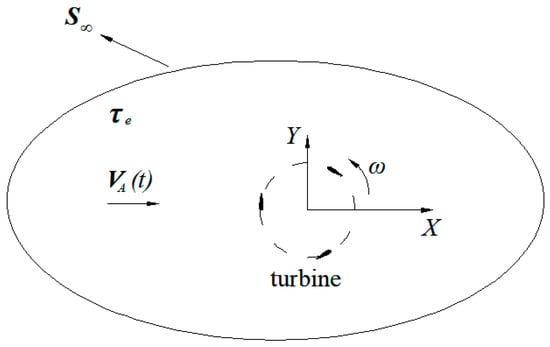
Figure 1.
The flow domain.
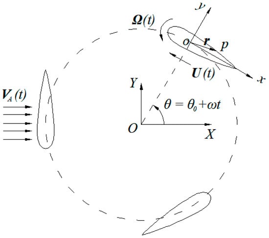
Figure 2.
Coordinate system and blade motion.
The velocity of uniform incoming flow is , which at infinity is
is the velocity potential at point p and time t, which meets the Laplace equation in the fluid domain :
and the non-penetration boundary condition on the blade surface:
where nb is the normal of the blade surface Sb; and r is the vector from the origin o to any surface point in the coordinate system xoy.
At infinity, satisfies the velocity potential for uniform incoming flow,
Introducing as the perturbation velocity potential, can be decomposed into two parts:
Assuming zero initial perturbation, should satisfy the following equation and boundary conditions:
The boundary element method is used to solve the time-discrete Laplace equations in combination with the Neumann boundary conditions as described by Equations (6)–(9). As shown in Figure 3 for the hth blade (h = 1,…, Z; Z is the number of turbine blades), sources are distributed on the blade surfaces , linear vortices γf(s) are placed along the arced centerline of the blade profile to generate lift force. A time-discrete vortex model is used to simulate trailing vortices , which are shed from the trailing edge and move at the local particle velocity, as shown in Figure 3. As a result, at an arbitrary point p in the fluid field, the induced velocity can be expressed as:
in which
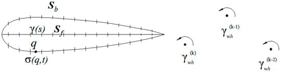
Figure 3.
Elements of the hth blade at time tk.
To compute Equation (10), we divide each blade surface Sb into N elements at which the sources (j = 1, N) are distributed, and surface Sf into M elements with a linear distribution. Assuming vorticity intensity at the leading edge and at the end of the arced centerline, the vorticity intensity on the surface Sf can then be described as:
at which is the length of the arced centerline. The total intensity of the vortices placed on Sf is:
With the movement of each blade after a time step Δt, a point vortex is generated at the trailing edge. As a result, a discrete vortex street is formed.
According to the surface boundary condition in Equation (7), Equation (10) for each surface element i can be discretized as
where Z is the number of blades, is the unit normal vector of the ith element on surface Sb and k represents the number of time steps at current time tk (tk = k × Δt).
In Equation (13), there are N × Z equations with (N + 3)Z unknown quantities, including the source strength of the N × Z element on the blade surfaces at current time tk, the vortex strength of Z blades, the vortex strength of newborn trailing vortices at the current moment and their positions . Thus, 3Z equations must be added to make Equation (13) close.
First, the Kutta condition of equal pressure is used on each blade to obtain Z equations, which can be expressed as:
That is, the pressure difference between the top and bottom surface of the airfoil trailing edge (T.E.) is zero. Applying the unsteady Bernoulli equation at an arbitrary point in the fluid field, the dynamic pressure P can be expressed as:
Applying Equation (15) to Equation (14) produces:
where is the pressure on the upper surface of the airfoil trailing edge, is the pressure on the lower surface of the airfoil trailing edge, is the perturbation velocity potential on the upper surface of the airfoil trailing edge, is the perturbation velocity potential on the lower surface of the airfoil trailing edge, is the vector of the upper surface of the airfoil trailing edge in the local body-fixed coordinate system and is the vector of the lower surface of the airfoil trailing edge in the local body-fixed coordinate system.
After obtaining the perturbation velocity on the blade surface unit numerically from Equation (10), the pressure distribution in each element can be calculated using the unsteady Bernoulli equation. Then, the hydrodynamic force on the airfoil blade can be obtained by numerical integration. The time derivative of the perturbation potential can be obtained by the finite difference method:
At any time , the perturbation velocity potential is determined by the line integral of the perturbation velocity . Theoretically, the starting point of the integral should be infinity. However, in actual calculation the starting point is 10 times the distance from the rotation center O of the water turbine. Integrating from the starting point to the rotation center O, then from O to the lower point of each trailing edge, the perturbation velocity potential of any element center in the whole airfoil can be derived:
where is the perturbation velocity potential at .
Second, the Kelvin condition is applied at each blade to obtain Z equations as follows:
where is the total intensity of vortices on Sf of the hth blade at time tk and is the total intensity at the preceding time step tk−1.
Third, the position of newborn trailing vortices of the hth blade at the current time can be determined as:
where is a constant coefficient, .
The blade surface pressure coefficient is defined as:
where ρ is the density of water. The resulting force on the blade is:
The moment on the blade reference point is:
The tangential force coefficient of the turbine blade is defined as:
and the normal force coefficient of the turbine blade as:
where is the turbine blade tangential force, is the turbine blade normal force, C is the turbine blade chord and b is the turbine blade length.
3. Results
3.1. Model Validation against Past Studies
Previously, many researchers have studied the hydrodynamic performance of vertical axis turbines. A representative study is Strickland’s model test study []. The parameters for one of the turbine models (Turbine A) in his work are shown in Table 1. The normal force, tangential force and wake evolution were also recorded in his experiment. Strickland’s test is often used as a benchmark for the validation of numerical models. In addition, there are a number of representative modeling studies, such as the FEVDTM proposed by Ponta [] and the CFD method proposed by Li []. This paper first compares the predictions from different methods with the turbine model given in Table 1.

Table 1.
Turbine model parameters (Strickland []).
In the numerical computation, the number of elements is chosen as N = 80, M = 40 and the time step is , where T is the rotation period of the turbine, T = 2π/ω; further fine mesh and smaller time step present very similar result. Figure 4 and Figure 5 compare the predicted central path of the turbine wake vortices from different studies for blade number Z = 1 and speed ratio λ = ωR/VA = 5. In Figure 4, the light streak shows the wake’s conformation obtained from Strickland’s model test using the dye injection visualization technique [] and the line with marked circles is the prediction result based on Ponda’s FEVDTM model []. Figure 5 demonstrates the result predicted by the method proposed in this paper. Comparing the results in Figure 4 and Figure 5, the turbine vortex wakes predicted by the proposed model are in good agreement with the experiment and the FEVDTM model.
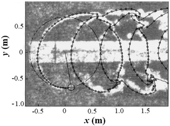
Figure 4.
Shed vortex central path by experimental visualization and FEVDTM prediction (Turbine A, λ = 5, Z = 1).
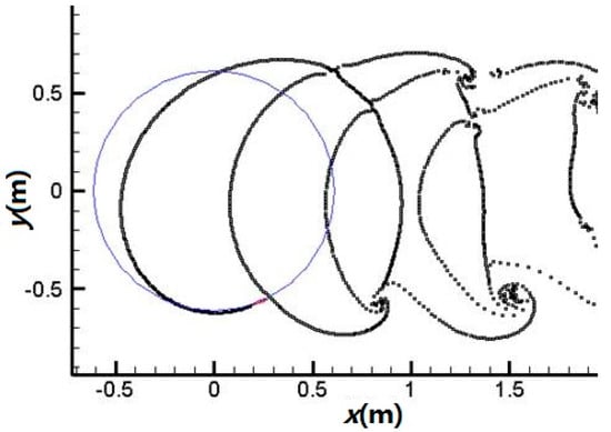
Figure 5.
Shed vortex central path predicted by the present study (Turbine A λ = 5, Z = 1).
Next, a quantitative comparison is carried out. The normal and tangential force coefficients against the azimuthal angle θ (as shown in Figure 2) of one blade of the turbine are calculated for the cases of Z = 2 and λ = 2.5, 5, 7.5. The results are presented in Figure 6, Figure 7 and Figure 8. The results from the experiment and the CFD model in the literature are also shown for comparison purposes. The quantitative results predicted by the present method agree with those predicted by Li’s CFD method [] and Strickland’s experiment []. Compared with the experimental test, the measured force at the peak and trough based on numerical methods is somewhat different. Overall, both the CFD and our method predict the normal force more accurately than the tangential force when compared with the experimental results. This may be attributed to either the tangled wake field of the turbines or ignoring the viscous effects of the fluid. However, the tangential force is one order lower than the normal force, so it has less impact on the performance analysis.
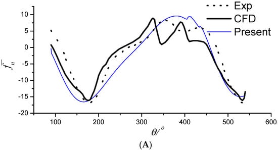
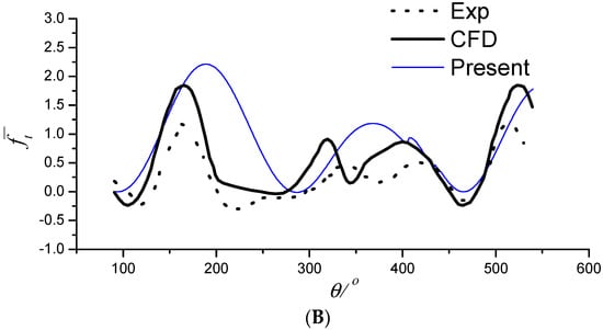
Figure 6.
(A) Normal force coefficient (λ = 2.5, Z = 2); (B) tangential force coefficient (λ = 2.5, Z = 2).
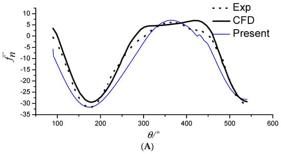
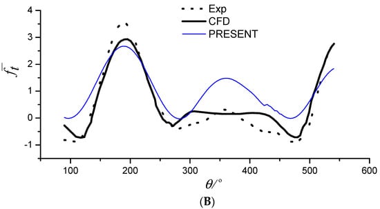
Figure 7.
(A) Normal force coefficient (λ = 5, Z = 2); (B) tangential force coefficient (λ = 5, Z = 2).
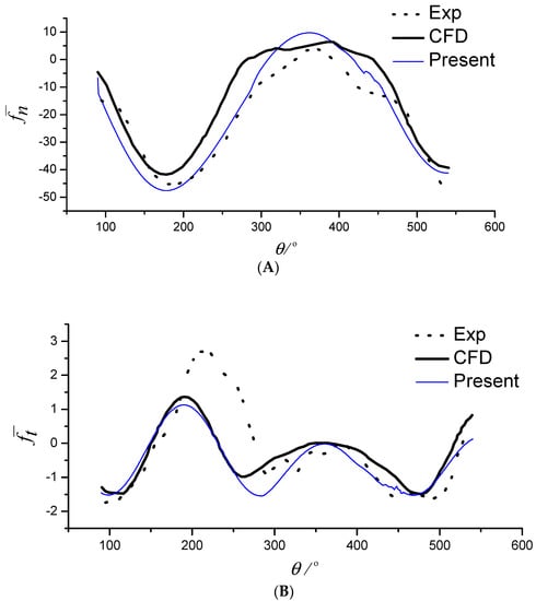
Figure 8.
(A) Normal force coefficient (λ = 7.5, Z = 2); (B) tangential force coefficient (λ = 7.5, Z = 2).
In the case of Z = 2, the total number of elements is 240, the time step is , the motion time is 4T including 1440 time steps and the computation time is only 15 min using a one-core 2.5 GHz CPU. The calculation time and computer memory needed by the proposed method are far less than the CFD method. Based on the above analyses and comparisons, it appears that the proposed method can satisfy the engineering requirements of fast prediction of turbine performance and hydrodynamic interference between multiple turbines in tidal power plants.
3.2. Comparison with a Laboratory Test
To study the hydrodynamic performance of the turbine further and validate the proposed method, a model test was conducted in a towing tank. The towing tank was 130 m long, 6 m wide and 4 m deep. The maximum speed of the trailer was 6.5 m/s. A vertical-axis turbine model was fixed on the trailer and then driven by it. The turbine was driven by a motor through the reduction gear box. Due to limited test conditions, only the torque of the hydraulic turbine model was measured. Figure 9 shows the apparatus used to measure the torque of the vertical-axis turbine: Figure 9A shows the test layout, Figure 9B the five-blade vertical-axis turbine model, Figure 9C the torque meter and Figure 9D a 32-channel dynamic data acquisition instrument. A torque meter was arranged between the turbine and the driving motor to measure the torque produced by the turbine at a given inflow speed and speed in real time. To avoid the influence of the free surface, the turbine was immersed below 0.4 m. The accuracy of the torque meter is 0.3%. The center of the torque meter is a strain shaft. The upper end of the strain shaft is the driving motor and the lower end is the turbine. When the turbine rotates and causes the strain shaft to be slightly deformed by torsion, the resistance value of the strain meter pasted on the strain shaft changes correspondingly. The change in strain resistance can be transformed into a change in voltage signal which is output to the dynamic data acquisition instrument, and the transient value of the hydraulic turbine torque can be obtained after the transformation.
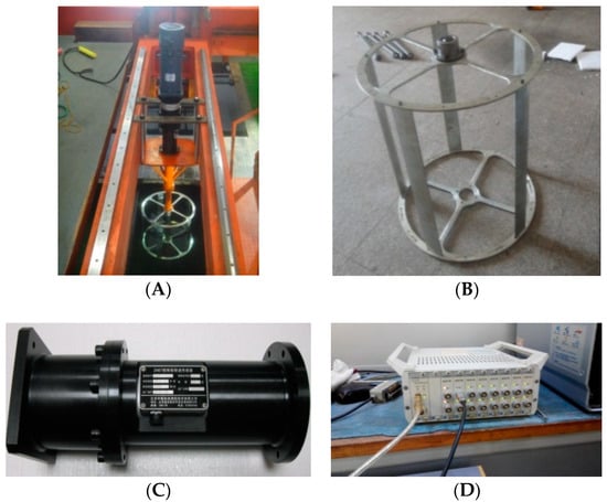
Figure 9.
Apparatus used to measure the torque of a vertical-axis turbine. (A) Test layout; (B) Five-blade vertical-axis turbine model; (C) Torque meter; (D) 32-channel dynamic data acquisition instrument.
The model parameters used in the experiment are listed in Table 2. Two models were tested: One with three blades and the other with five blades. To match operating conditions of the vertical-axis tidal current turbine power station in Guanshan Island, Zhoushan, China, two typical speed ratios were selected for each turbine model: 1.6 and 2.2 for the three-blade model and 1.65 and 2.23 for the five-blade model. The torque test results Q can be transformed into a torque coefficient , where D is the turbine diameter. The torque coefficient against the azimuthal angle θ after the third revolution for two different turbine models and speed ratios predicted by the proposed method are shown in Figure 10, Figure 11, Figure 12 and Figure 13. Figure 10 and Figure 11 show that the torque coefficient curve for a turbine with three blades has three peaks in one cycle, while Figure 12 and Figure 13 show that a five-blade turbine produces five peaks. The number of peaks in one cycle is related to the number of blades. Overall, the computed results are in good agreement with those obtained from experiments, which indicates that the model can capture the torque performance of the turbine well. However, a difference in the peaks and valleys is observed, which may be attributed to the following reasons. First, the proposed method is based on potential flow theory, in which the viscous effect is ignored. Second, it is a two-dimensional model and the experiment is carried out under three-dimensional conditions. These effects will be investigated in greater depth in future studies.
Table 2.
Parameters of the model test.
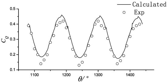
Figure 10.
Turbine B (V = 1.2, λ = 1.6, Z = 3).
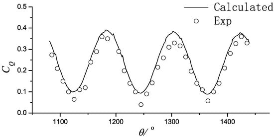
Figure 11.
Turbine B (V = 1.2, λ = 2.2, Z = 3).
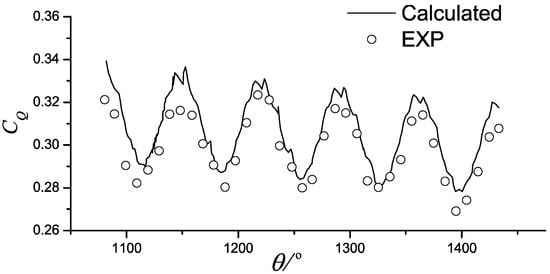
Figure 12.
Turbine C (V = 1.2, λ = 1.65, Z = 5).
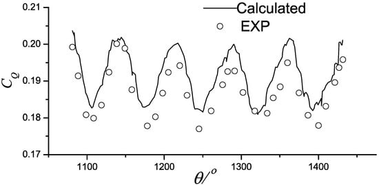
Figure 13.
Turbine C (V = 1.2, λ = 2.23, Z = 5).
4. Conclusions
In this paper, the flow induced by the motion of the vertical-axis turbine has been simplified as a two-dimensional problem and solved using the unsteady boundary element method. A code for the proposed method was developed specifically for performance analysis of vertical-axis turbines. In comparison with previous studies, the proposed model is simpler and more efficient. It can capture our experimental results well and satisfy the engineering application requirements for performance prediction of vertical-axis turbines. The results imply that the proposed method can be adopted as a tool for analyzing the hydrodynamic performance of vertical-axis tidal turbines. The code developed provides a useful design tool for optimizing the airfoil profile and arrangement of tidal power devices. In this study, we ignored the viscous effect of the fluid and an uncertainty analysis was not carried out. These will be incorporated in our future research and may lead to a better prediction. Another future research direction is to develop the method to solve three-dimensional problems.
Author Contributions
G.L.: Contribution to the research conception, literature search, model established, data collection, analysis, and interpretation, manuscript writing; Q.C.: Literature search, figures, study design, data analysis and interpretation, manuscript writing and revision; H.G.: Data analysis, data interpretation, revision and communication etc.
Funding
The study was supported by the National Natural Science Foundation Program (51679216), and by the Open Research Foundation of Key Laboratory of the Pearl River Estuarine Dynamics and Associated Process Regulation, Ministry of Water Resources.
Conflicts of Interest
The authors declare no conflicts of interest.
References
- Bilgen, S.; Keles, S.; Kaygusuz, A. Global warming and renewable energy sources for sustainable development: A case study in Turkey. Renew. Sustain. Energy Rev. 2008, 12, 372–396. [Google Scholar] [CrossRef]
- Li, Z. Numerical Simulation and Experimental Study on Hydrodynamic Characteristic of Vertical Axis Tidal Turbine. Ph.D. Thesis, Harbin Engineering University, Harbin, China, 2011. [Google Scholar]
- Lv, X.; Qiao, F. Advances in study on tidal current energy resource assessment methods. Adv. Mar. Sci. 2008, 1, 98–108. [Google Scholar]
- Camporeale, S.M.; Magi, V. Stream tube model for analysis of vertical axis variable pitch turbine for marine currents energy conversion. Energy Convers. Manag. 2000, 41, 1811–1827. [Google Scholar] [CrossRef]
- Zhang, L.; Wang, L.; Li, F. Stream tube models for performance prediction of vertical-axis variable-pitch turbine for tidal current energy conversion. J. Harbin Eng. Univ. 2004, 25, 261–265. [Google Scholar]
- Coiro, D.P.; Nicolosi, F. Numerical and experimental analysis of kobold turbine. In Proceedings of the Synergy Symposium on Vertical Axis Wind Turbine, Hangzhou, China, 24 November 1998; pp. 4–6. [Google Scholar]
- Ladopoulos, E.G. Non-linear multidimensional singular integral equations in two-dimensional fluid mechanics. Int. J. Non-Linear Mech. 2000, 35, 701–708. [Google Scholar] [CrossRef]
- Ponta, F.L.; Jacovkis, P.M. A vortex model for Darrieus turbine using finite element techniques. Renew. Energy 2001, 24, 1–18. [Google Scholar] [CrossRef]
- Li, Y. Development of a Procedure for Predicting the Power Output from a Tidal Current Turbine Farm. Ph.D. Thesis, University of British Columbia, Vancouver, BC, Canada, 2008. [Google Scholar]
- Hwang, I.S.; Lee, Y.H.; Kim, S.J. Optimization of cycloidal water turbine and the performance improvement by individual blade control. Appl. Energy 2009, 86, 1532–1540. [Google Scholar] [CrossRef]
- Ferreira, C.S.; Scarano, F.; Bussel, G.V.; Kuik, G.V. 2D CFD simulation of dynamic stall on a vertical axis wind turbine: Verification and validation with PIV measurements. In Proceedings of the 45th AIAA Aerospace Sciences Meeting and Exhibit, Reno, Nevada, 8–11 January 2007. [Google Scholar]
- Li, F.; Jiang, D.; Meng, Q. Study on the self starting performance of the fixed straight bladed vertical axis tidal turbine. Eng. Test. 2011, 9, 23–26. [Google Scholar]
- Li, Z.; Zhang, X.; Zhang, L. Experimental study on blade preset position of fixed pitch vertical axis tidal turbine. Renew. Energy Resour. 2012, 30, 37–41. [Google Scholar]
- Stallard, T.; Collings, R.; Feng, T. Interactions between tidal turbine wakes: Experimental study of a group of three-bladed rotors. Philos. Trans. R. Soc. 2013, 371. [Google Scholar] [CrossRef] [PubMed]
- Strikland, J.H. The Darrieus Turbine: A Performance Prediction Model Using Multiple Streamtubes; Sandia Laboratory Rept. SAND 75-0431; Sandia National Laboratories: Albuquerque, NM, USA, 1975. [Google Scholar]
© 2018 by the authors. Licensee MDPI, Basel, Switzerland. This article is an open access article distributed under the terms and conditions of the Creative Commons Attribution (CC BY) license (http://creativecommons.org/licenses/by/4.0/).