Soil Erosion Modeling and Comparison Using Slope Units and Grid Cells in Shihmen Reservoir Watershed in Northern Taiwan

Abstract

Soil erosion is a global problem that will become worse as a result of climate change. While many parts of the world are speculating about the effect of increased rainfall intensity and frequency on soil erosion, Taiwan’s mountainous areas are already facing the power of rainfall erosivity more than six times the global average. To improve the modeling ability of extreme rainfall conditions on highly rugged terrains, we use two analysis units to simulate soil erosion at the Shihmen reservoir watershed in northern Taiwan. The first one is the grid cell method, which divides the study area into 10 m by 10 m grid cells. The second one is the slope unit method, which divides the study area using natural breaks in landform. We compared the modeling results with field measurements of erosion pins. To our surprise, the grid cell method is much more accurate in predicting soil erosion than the slope unit method, although the slope unit method resembles the real terrains much better than the grid cell method. The average erosion pin measurement is 6.5 mm in the Shihmen reservoir watershed, which is equivalent to 90.6 t ha⁻¹ yr⁻¹ of soil erosion.

1. Introduction

Soil erosion is the detachment of soil particles occurring in a landscape. Compared with wind erosion, water erosion is a much more critical process that produces enormous sediments in Taiwan’s watersheds. There are many factors that contribute to the high soil erosion rate of Taiwan. The first and foremost is Taiwan’s hilly topography. Situated at the collision boundary of the continental Eurasian plate and the Philippine Sea plate, the mountain range of Taiwan is being lifted at a rate of 0.2–18.5 mm yr⁻¹ [1], which creates some of the most rugged terrain in East Asia. The second problem is Taiwan’s thick soil deposits due to heavy weathering as a consequence of the island’s tropical to subtropical weather. Finally, the last problem that exacerbates the soil erosion conditions in Taiwan is the heavy rain brought by monsoons and typhoons. Due to the amount and intensity of the rainfall, the rainfall erosivity value of Taiwan is many times higher than the global average obtained by Borrelli et al. [2], making water erosion a very serious concern in Taiwan. In fact, not just in Taiwan, the concern of soil erosion has been evident in many published studies in different parts of the world, including Europe [3,4], the US and Mexico [5,6], mainland China [7,8], India [9,10], Africa [11,12], Australia [13,14], etc. A steady increase in the number of studies on soil erosion in the last few years has also prompted a few regional and global studies that provide a bigger picture of the emerging crisis [2,15,16,17]. If we factor in the threat of climate change, we will likely face more intense precipitation occurring at a higher frequency in the near future. In order to be prepared for the possible global increase in soil erosion, studying existing high soil erosion areas such as Taiwan’s watersheds may provide insights into a preventive measure against a massive increase of global soil loss.

In this study, we selected a representative watershed in Taiwan as the study area. The watershed was monitored by 550 erosion pins installed at 55 locations from 8 September 2008 to 10 October 2011. Two variations (grid cells and slope units) of the soil erosion model based on the universal soil loss equation (USLE) were used to compute the soil loss due to sheet and rill erosion. The results will be compared with the measurement of erosion pins in different sub-watersheds. For the purpose of this research, we assume that the data layers used in the analysis are representative of the study area even though the data were not gathered at the same time. The goals are to examine the difference between a grid cell analysis and an analysis based on natural land boundaries (slope units), and to determine which is more accurate in predicting erosion pin measurements.

2. Materials and Methods

This study took a modeling and validation approach. That is, we first developed a model to estimate the amount of soil erosion. Then, we validated the model using field measurements of erosion pins. The soil erosion model that we built is based on the digital elevation model (DEM) acquired by the Central Geological Survey (CGS) of Taiwan in 2013 with airborne LiDAR (light detection and ranging). The horizontal resolution of the DEM was 10 m. The soil erosion was computed using the USLE with two different analysis units: grid cells and slope units.

2.1. Universal Soil Loss Equation

The universal soil loss equation (USLE) was used to compute the sheet and rill erosion by water. Despite its shortcomings, the USLE and its successor RUSLE (Revised Universal Soil Loss Equation) is still the most common soil erosion model for data scarce catchments. It is reported that at least 90% of soil erosion studies conducted worldwide use RUSLE-based models [18]. According to Wischmeier and Smith, the USLE “is an erosion model designed to compute longtime average soil losses from sheet and rill erosion” [19]. The equation is (in metric units):

$$A_m=R_m\times K_m\times \mathrm{L}\times \mathrm{S}\times \mathrm{C}\times \mathrm{P}$$

(1)

where

• Am = computed soil loss per unit area (t ha⁻¹ yr⁻¹)
• Rm = rainfall and runoff factor (MJ-mm ha⁻¹ hr⁻¹ yr⁻¹)
• Km = soil erodibility factor (t-hr MJ⁻¹ mm⁻¹)
• L = slope-length factor
• S = slope-steepness factor
• C = cover and management factor
• P = support practice factor

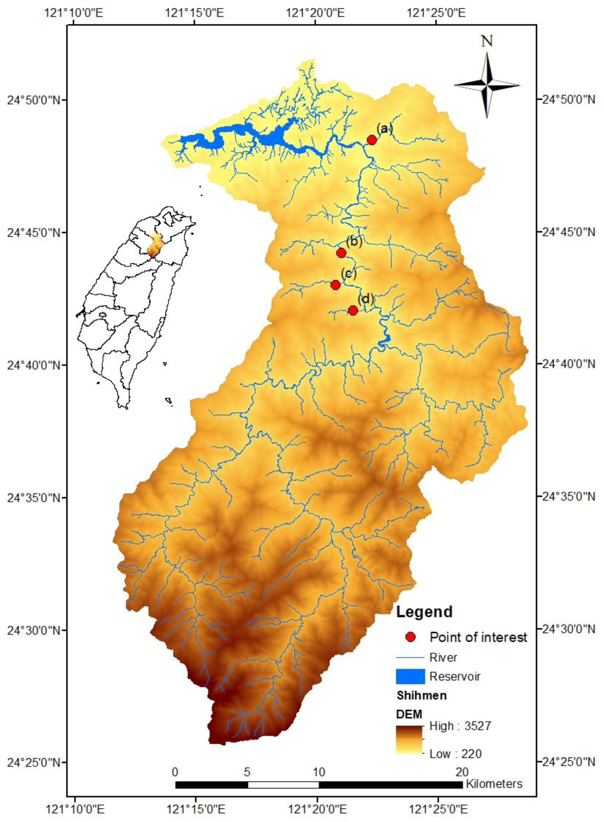
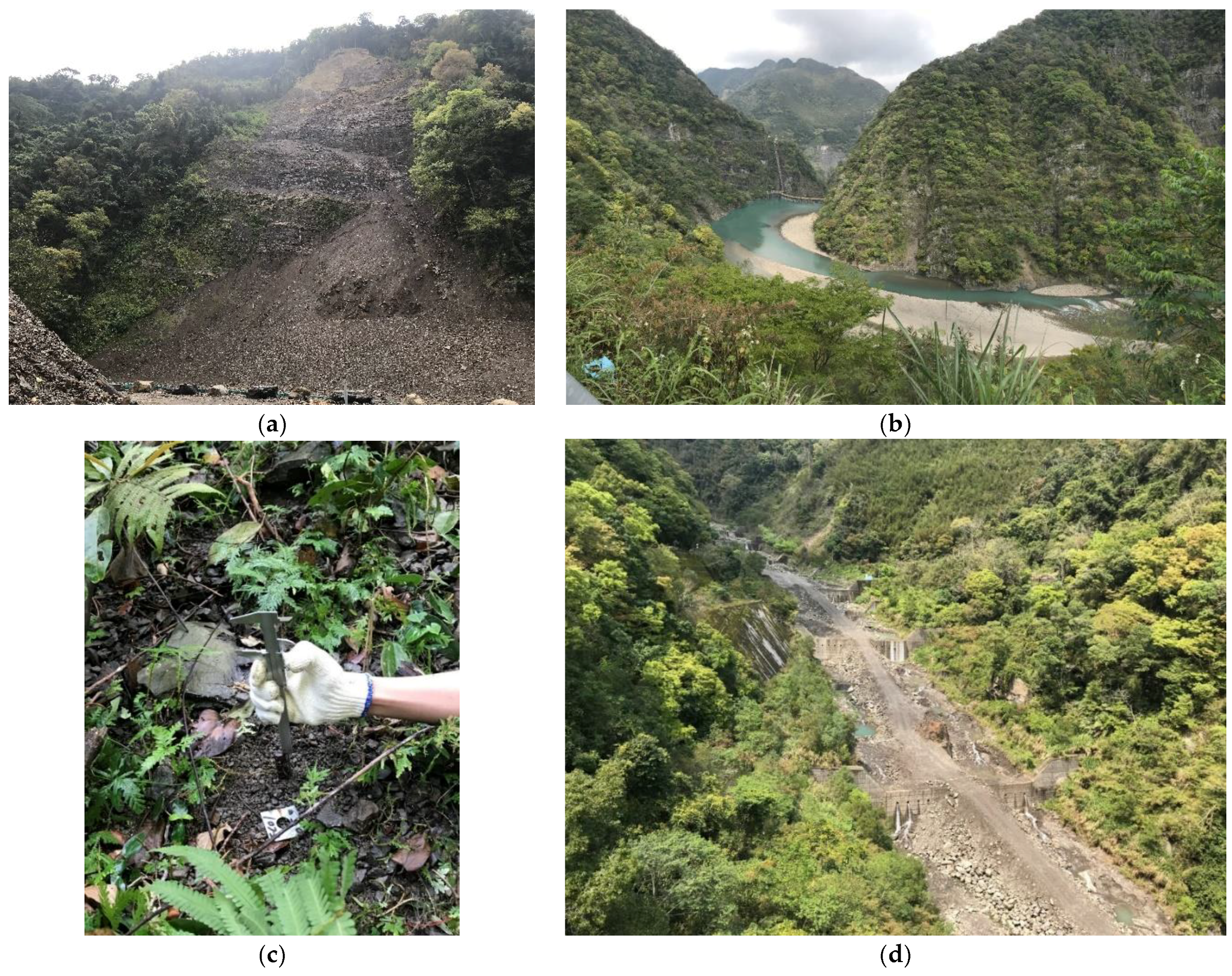
2.2. Study Area

The Shihmen reservoir watershed in northern Taiwan was selected as the study area. The reservoir itself is the third largest in Taiwan, and was constructed with an earth-and-rock fill embankment. As the reservoir supplies municipal, industrial, and irrigation water to northern Taiwan, it is often the focus of public attention. The location of the Shihmen reservoir watershed is shown in Figure 1. Marked on Figure 1 are the locations of field observations as photographed on 16 March 2018. Figure 2a is an example of soil erosion turned into a shallow landslide near the Hsia-Yun Creek after typhoon Nesat in 2017. The site also exhibits a typical recurrence of the alternation of erosion and landslides, which are common in the area. Figure 2b shows the Ronghua Dam, which is situated 27 km upstream of the Shihmen reservoir, and was constructed in 1983 with a capacity of 12.4 million m³. The Ronghua Dam serves as a hydropower facility, but its main function was as a check dam to protect the Shihmen reservoir (Shihmen Dam). As can be seen from Figure 2b, the Ronghua Dam (at the junction of two mountains near the center of the image) is almost filled with sediments. Figure 2c is one of the 55 sites monitored with erosion pins (10 pins per site) near Bao-Li-Ku Creek. The measurements were taken with a caliper. A detailed description of the installation of the erosion pins can be found in Lin et al. [20]. Finally, Figure 2d shows a series of check dams at Su-Le Creek. The check dams are filled with sediments and have completely lost their protection function. As can be seen from these field photos, the sediment problem in the Shihmen reservoir watershed is very alarming, and a good model for estimating the amount of soil erosion in the watershed is crucial.

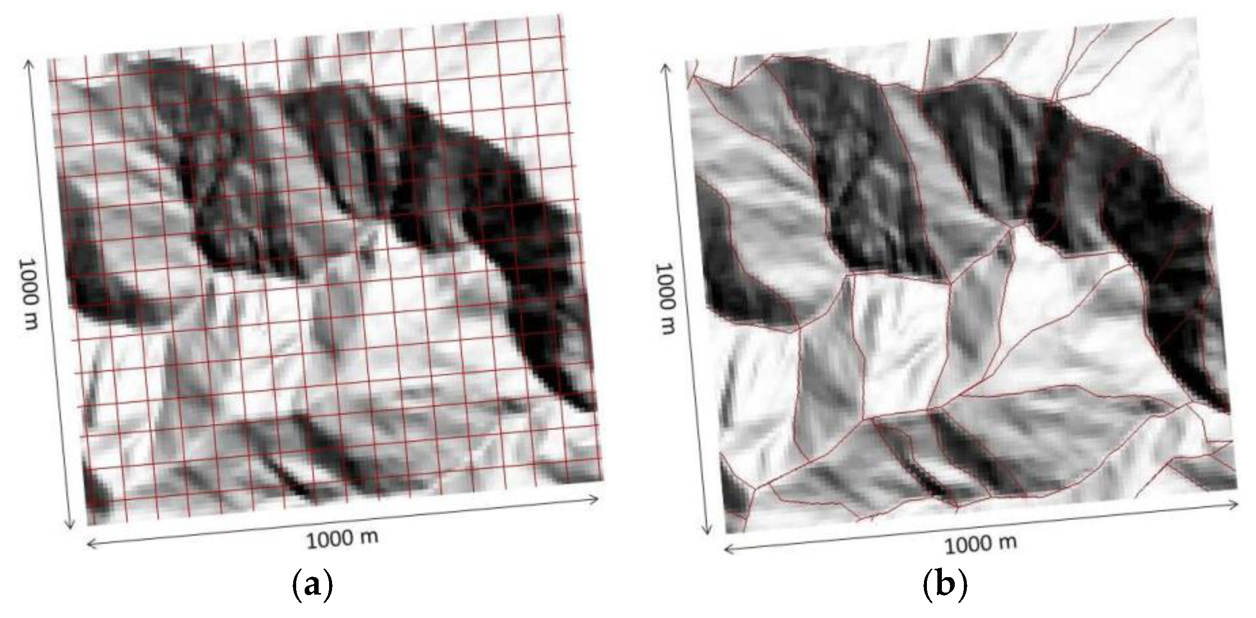
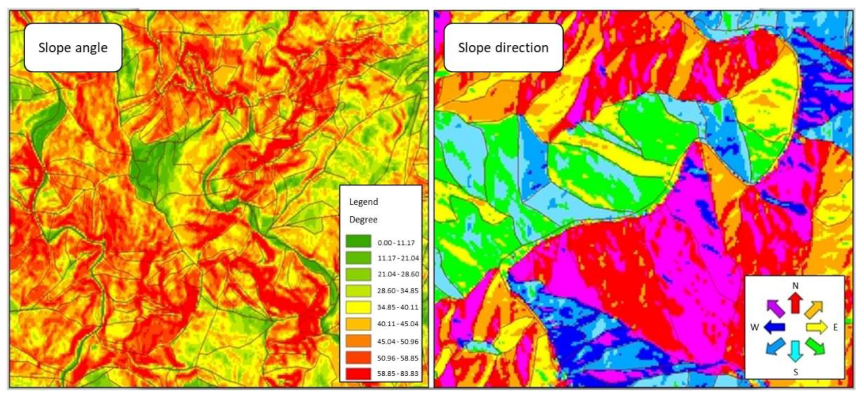
2.3. Grid Cells and Slope Units

In this study, the rainfall factor R was obtained from Lu et al. [21], and the soil erodibility factor K was obtained from Wann and Hwang [22]. The average R factor was 12,798 MJ-mm ha⁻¹ hr⁻¹ yr⁻¹, or 6.4 times the global average of 2000 MJ-mm ha⁻¹ hr⁻¹ yr⁻¹ [23]. The K factor ranged from 0.004 to 0.042 t-hr MJ⁻¹ mm⁻¹ [24]. The C factor was converted from a land use survey in 2004 [25] and a conversion table between the land uses and the C factors [26], and the average C value was 0.016. Finally, the P factor was assumed to be 1, as is usually done in the literature when there are no protection measures.

The topographic factors L and S were derived from the CGS DEM. They were computed using Equations (2) and (3) from [19]:

$$\mathrm{L}={\left(\frac{\lambda }{22.13}\right)}^m$$

(2)

where

• λ = slope length in meters
• m = 0.5 if percent slope is 5% or more
•    = 0.4 on slopes of 3.5% to 4.5% [19] or 3% to 5% [26]
•    = 0.3 on slopes of 1% to 3%
•    = 0.2 on uniform gradients of less than 1%

$$\mathrm{S}=65.41{sin}^2\theta +4.56sin\theta +0.065$$

(3)

where

• θ = the angle of slope

The original USLE handbook makes no reference to measuring the slope length in horizontal projection [19,27], but the RUSLE handbook specifically specifies such measurements [28]. Some studies (such as Oliveira et al. [29]) use slope lengths parallel to the surface in their computations.

GIS (Geographic Information System) and soil erosion modeling usually go hand in hand, especially for large areas. As the study area is too vast to be covered in a single plot or unit, the Shihmen reservoir watershed is divided into many smaller units to facilitate computation and analysis. In GIS, the easiest way to accomplish the division of a study area is by using square grid cells, as shown in Figure 3a. Many spatial analysis tools in GIS support the use of gridded datasets. It is a superior method to a station-based approach, but could sometimes provide misleading information [30]. Still, many studies of soil erosion use grid cells in their analysis [9]. On the other hand, the grid cells do not conform to any natural land boundaries and the results may be biased. This is especially problematic for computing the slope-length factor L, which is the most difficult factor to calculate among the six factors of the USLE. To approximate the shape of the hillslopes and compute the slope length λ in Equation (2), different methods have been proposed, such as Hickey [31] and Sextante [32], the unit contributing area [33,34], and a combination of the unit contributing area and LS-TOOL [35]. In addition, Foster and Wischmeier [36] propose dividing a slope into segments.

In this study, the first approach used was the grid cell method. We first assumed that hillslopes could be divided into uniform 10 m by 10 m squares, and the amount of soil erosion could be evaluated on a cell-by-cell basis. For the slope length factor, two kinds of procedures were employed to calculate the slope lengths—in directions parallel to the slope surfaces [29] and in a horizontal projection. Then for contrast, we relaxed the assumption regarding the computing soil erosion of each cell individually, and used the SAGA (System for Automated Geoscientific Analyses) software to calculate the LS factors.

To contrast the grid cell approach and be more representative of the field situation, slope units (sometimes called terrain units) were also used in this study. In contrast to grid cells, slope units are based on natural terrains of the study area, as shown in Figure 3b. The natural water divides between distinct geographic areas were used as the boundaries of the units. In this method, each slope unit is a close representation of an individual slope, which makes the application of the USLE more suitable. Note that the slope units depend on the breaks of topography. The soil properties and groundwater conditions may be the same or very similar between adjacent units.

Both approaches have their respective advantages and disadvantages. For the grid cell approach, its advantage lies in its simplicity and applicability. However, it is too restrictive on the slope length for the assumption that we made. On the other hand, the slope unit approach places no restriction on the length of the slope, but the approach is difficult to implement and automate. In this study, both the grid cell approach and the slope unit approach were used, and their results were compared. Since the grid cell approach is commonly used in GIS analysis, it does not require further explanation. The following will explain how slope units were delineated in this study.

Although rarely used in soil erosion, the slope unit approach has often been applied to the study of landslides. The slope units were created by inverting the DEM to intersect with the original DEM. The intersections form the required slope units [37]. Unfortunately, the procedure is not fool-proof, and it requires manual inspection and editing. The editing includes the correction of slope angles and slope directions (Figure 4), removal of peculiar areas (Figure 5), filling in of missing areas (Figure 6), and disregarding shadowed areas and river surfaces (Figure 7). The use of slope units is also called the object-oriented approach [18,38].

3. Results

This is the first time that a slope unit-based approach is applied to soil erosion modeling in the Shihmen reservoir watershed. The outcomes are interesting compared to the grid cell approach (10 m by 10 m). Here we will discuss our findings in four parts.

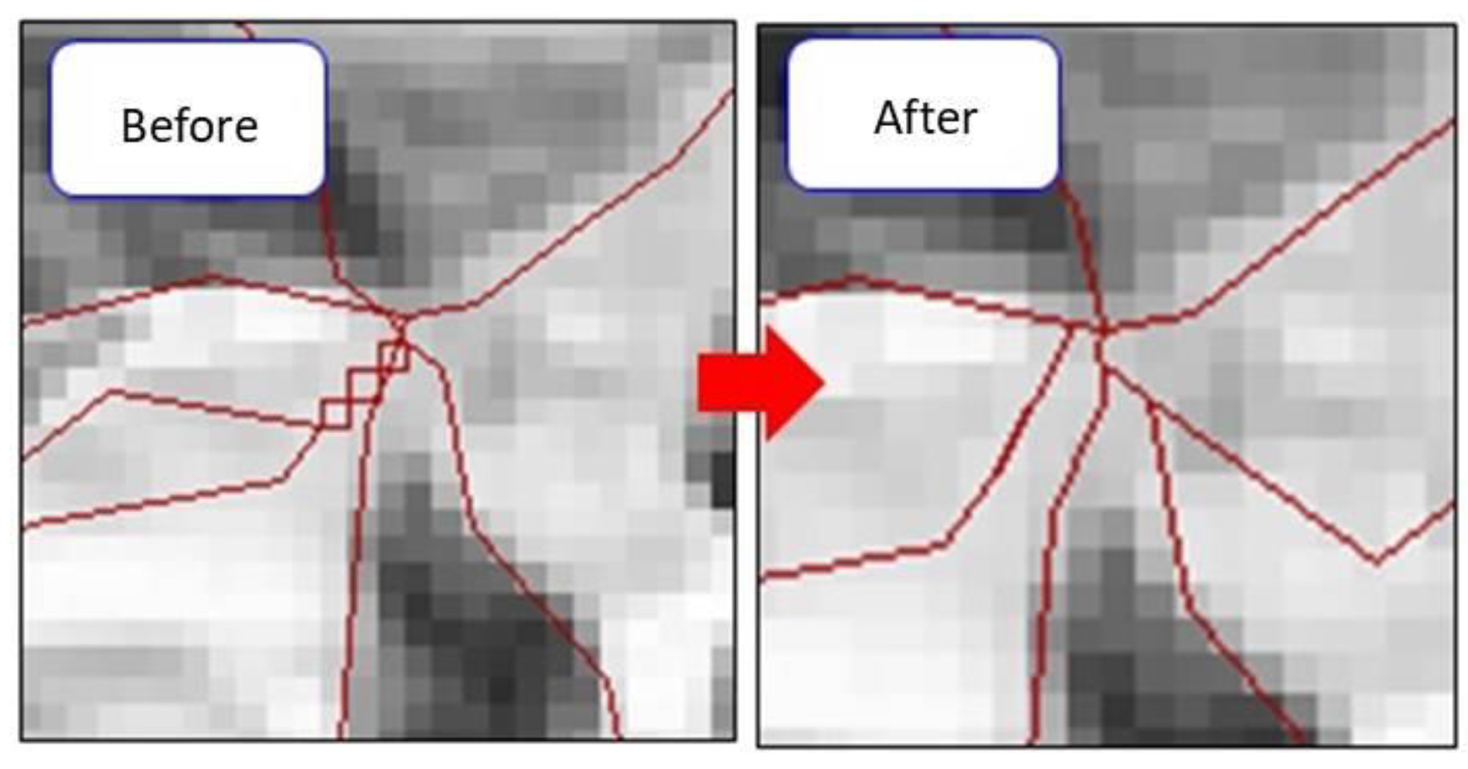
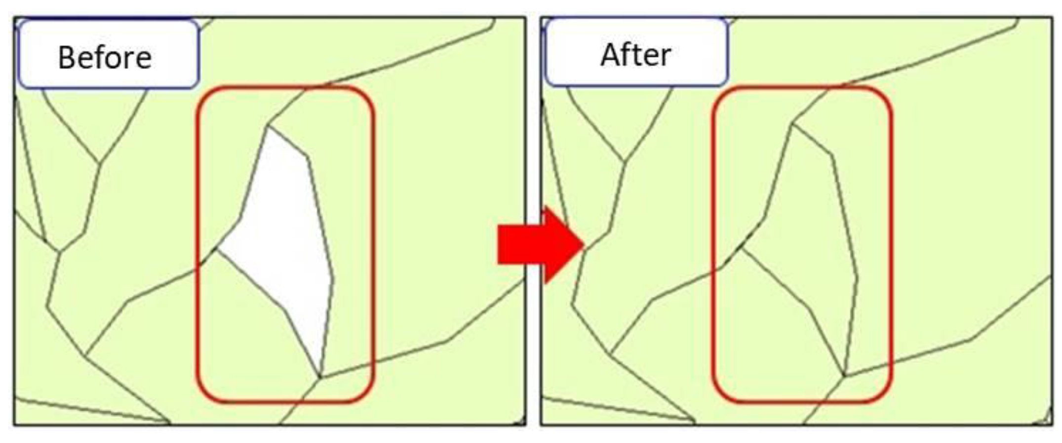
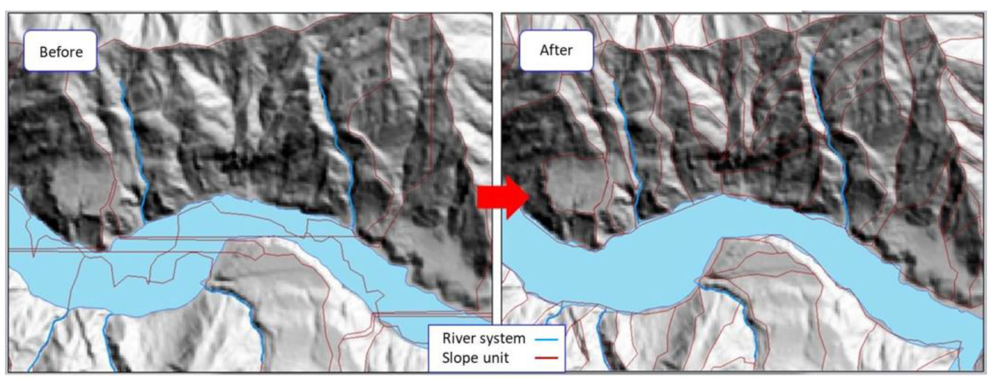
3.1. Delineation of the Study Area

The result of the delineation of the slope units is shown in Figure 8. All in all there are 19,275 slope units generated in the Shihmen reservoir watershed with an average size of 3.87 ha. It is obvious from Figure 8 that the slope units form a more realistic representation of the terrain of the study area. Therefore, the subsequent modeling of soil erosion based on slope units is likely to be more convincing.

3.2. Comparison of Topographic Factors L and S

The statistics of the L and S factors are shown in

Table 1. Comparison of L and S factors between grid cell approach (original) and slope unit approach.

Type		L	S
Grid cells	Max.	2.24	69.26
	Min.	0.67	0.07
	Mean	0.82	25.08
Slope units	Max.	7.47	56.24
	Min.	1.16	0.39
	Mean	3.05	25.70

. Two important observations can be made. First, the ranges and the averages of the S factors were almost the same for both approaches. This is reasonable in that the steepness of a slope should not be altered simply due to the shape or the size of the unit of analysis (at least not significantly). This intuition was supported by our results. Second, as anticipated, the slope length factors (L) were considerably different for both approaches. As shown in Table 1, the average L derived from the slope units was 3.7 times the average L of the grid cells. As USLE is multiplicative, the L factor alone could increase the amount of soil erosion to 3.7 times of the original amount.

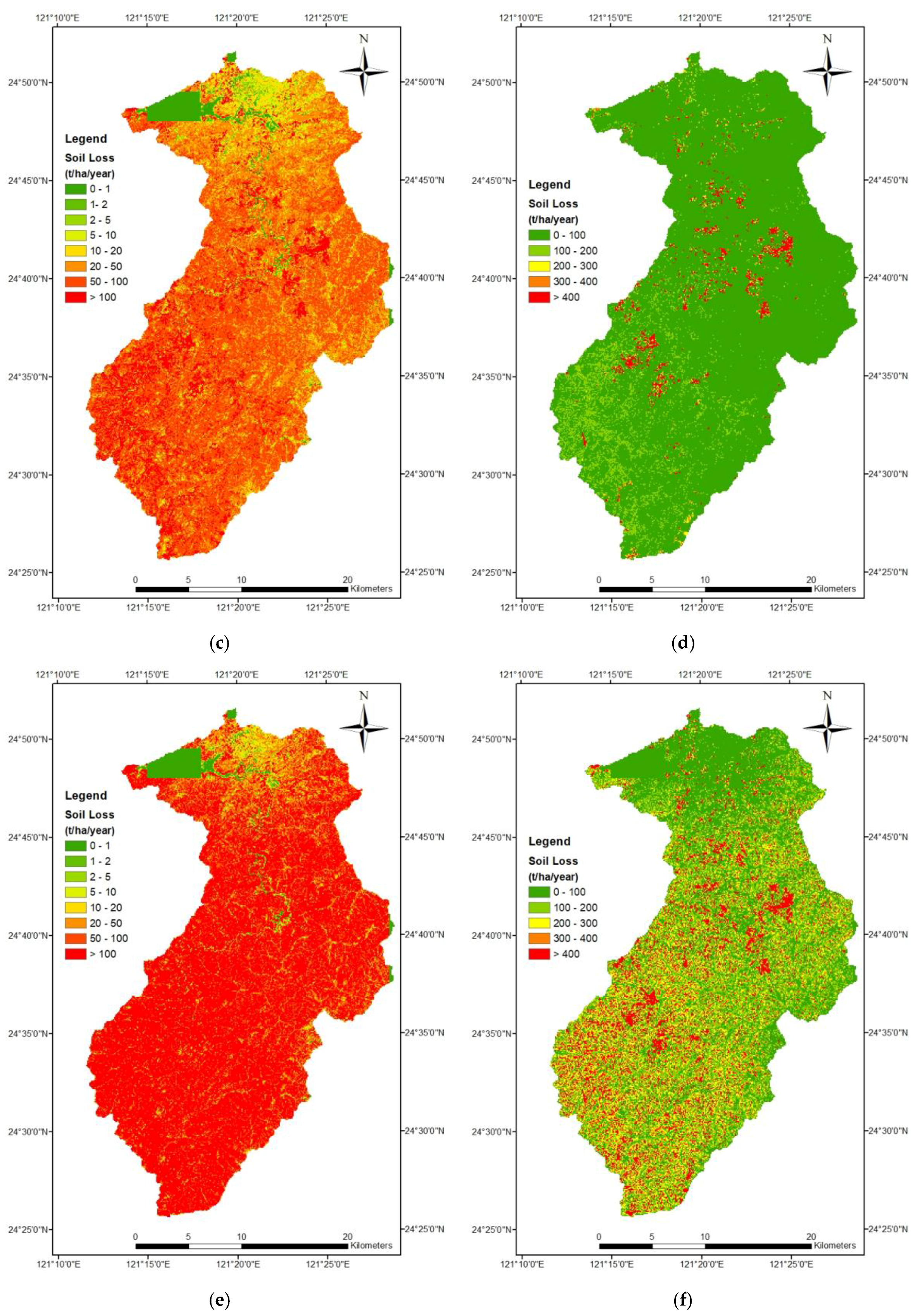
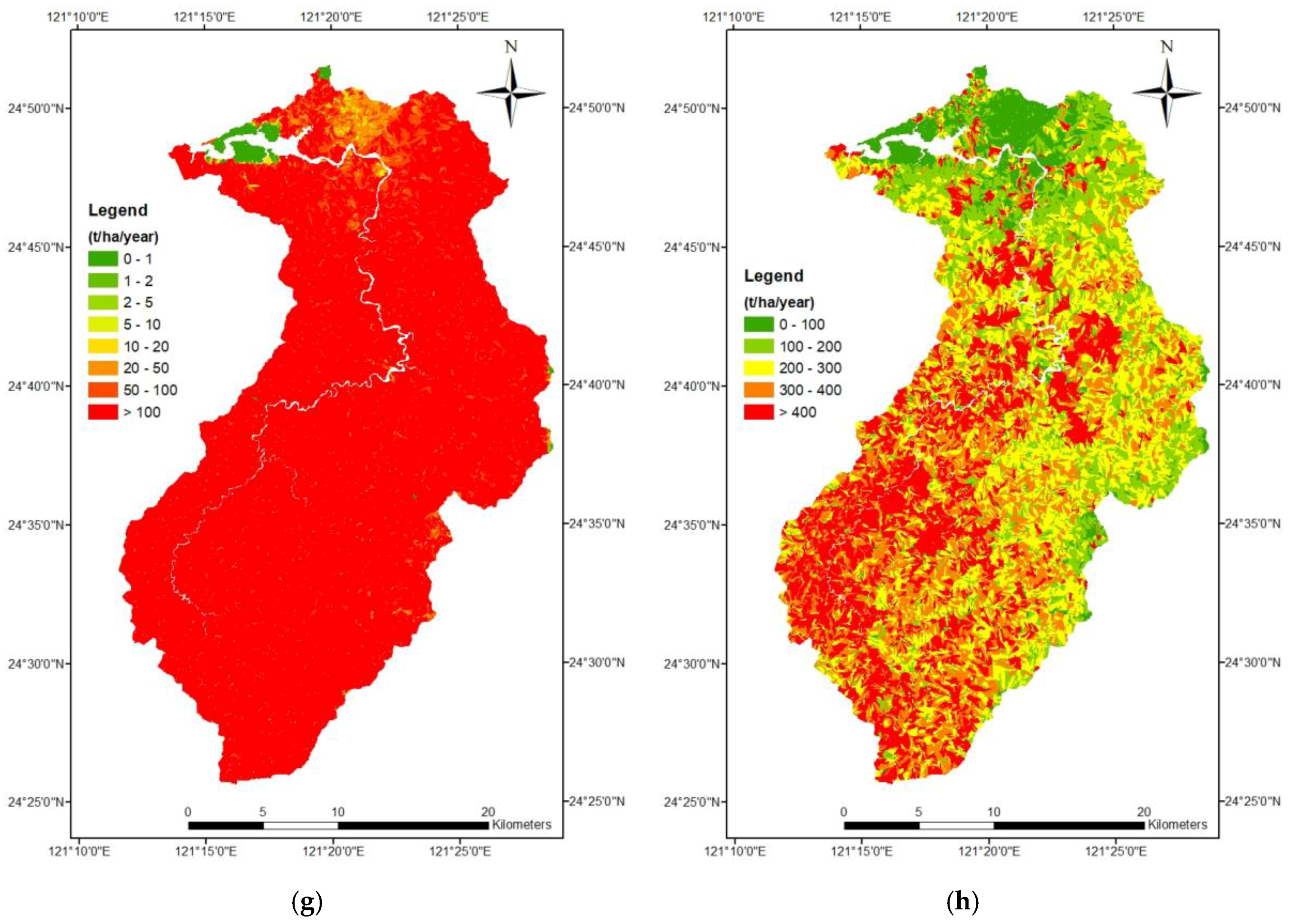
3.3. Comparison of Soil Erosion

The computed amounts of soil erosion for (1) the grid cell approach; (2) the grid cell approach with a horizontal projection; (3) the grid cell approach using SAGA; and (4) the slope unit approach are shown in Figure 9 using the internationally accepted scale (a, c, e, g) and our own classes (b, d, f, h). As can be seen from Figure 9, the result of the grid cells was pixel-like, whereas the result of the slope units was irregular in shape. All approaches show that the study area has high soil erosion, but the amounts of soil erosion are different. The average amount of soil erosion for the grid cell approach was 97.0 t ha⁻¹ yr⁻¹; for the grid cell approach with a horizontal projection it was 82.1 t ha⁻¹ yr⁻¹; for the grid cell approach using SAGA it was 280.1 t ha⁻¹ yr⁻¹; and for the slope unit approach it was 416.5 t ha⁻¹ yr⁻¹. In other words, the slope unit method has an amount of soil erosion 4.3 times higher than the grid cell approach. Since most of the remaining five USLE factors are similar in value, this result is in line with the observed ratio of 3.7 between the average L factors of the two approaches.

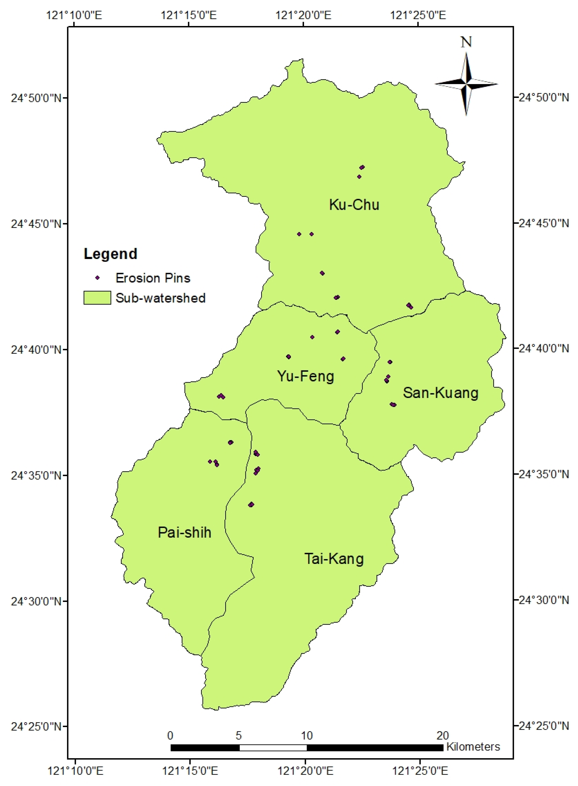
3.4. Validation with Erosion Pin Measurements

Figure 10 shows the distribution of the 55 sites monitored by erosion pins (10 pins per site), and

Table 2. Comparison of erosion pin measurements and predictions made by the grid cell approach and the slope unit approach.

	Erosion pins (mm)	Grid cell approach (mm)	Grid cell with a horizontal projection (mm)	Grid cell using SAGA (mm)	Slope unit approach (mm)
Ku-Chu sub-watershed	6.0	5.4	4.7	15.4	24.0
Yu-Feng sub-watershed	4.7	9.2	7.9	26.4	44.0
San-Kuang sub-watershed	8.9	5.2	4.4	15.6	25.6
Pai-Shih sub-watershed	6.4	10.1	8.8	30.9	46.8
Tai-Kang sub-watershed	6.8	7.0	5.9	20.2	31.2
Entire Shihmen reservoir watershed	6.5	6.9	6.0	20.3	29.8

shows the averages of the erosion pin measurements from 8 September 2008 to 10 October 2011 [39]. We divided the entire Shihmen reservoir watershed into five smaller sub-watersheds as shown in Figure 10. The sub-watersheds are Ku-Chu, Yu-Feng, San-Kuang, Pai-Shih, and Tai-Kang sub-watersheds. Then, we computed the average depth of the soil erosion in each sub-watershed using both the grid cell approach and the slope unit approach in Equation (4):

$$\mathrm{d}=\frac{A_t}{area\times \gamma }$$

(4)

where

• At = total amount of soil erosion (t)
• d = erosion depth (mm)
• area = area of watershed (ha)
• γ = unit weight of soil (t m⁻³)

The results are shown in Table 2. Here we assume γ = 1.4 t m⁻³ to compute the equivalent erosion depths in each sub-watershed and the entire Shihmen reservoir watershed. As can be seen from Table 2, the erosion depth of the entire Shihmen reservoir watershed computed by the grid cell approach is very close to the average measurement at the erosion pins (6.9 mm vs. 6.5 mm), whereas the erosion depth computed by the slope unit method was many times over the average erosion pin measurement. Individually speaking, the grid cell method was good in some sub-watersheds (the Ku-Chu sub-watershed and Tai-Kang sub-watershed) but not so good in the others (the Yu-Feng sub-watershed, San-Kuang sub-watershed, and Pai-Shih sub-watershed). If we convert the measured average erosion depth to the amount of soil erosion, 6.5 mm is equivalent to 90.6 t ha⁻¹ yr⁻¹.

4. Discussion and Conclusions

In this study, we modeled the soil erosion of the Shihmen reservoir watershed in northern Taiwan with two different analysis units, both of which were based on a 10 m resolution DEM acquired through airborne laser scanning. The first was a grid cell approach, and the second was a slope unit approach. As grid cells do not resemble real terrain, it was anticipated that the slope unit approach would substantially improve the estimation of soil erosion. However, contrary to our expectations, the result was the opposite. The grid cell method predicted an average erosion depth of 6.9 mm, very close to the actual average erosion depth of 6.5 mm (based on erosion pin measurements at 55 locations). On the other hand, the slope unit method yielded an average L factor 3.7 times the average L factor of the grid cell method, and the slope unit method produced an average amount of soil erosion 4.3 times higher than that of the grid cell method. Note that the grid cell approach using SAGA also did not yield results closer to the measured erosion depths. A cut-off slope angle of 50% or 55% was suggested by McCool et al. [40], Liu et al. [41], and Panagos et al. [34], but was not carried out in this study.

In addition, when we examined the five sub-watersheds of the Shihmen reservoir watershed, we observed good matches between the predictions of the grid cell method and the measurement of the erosion pins for some sub-watersheds but not others. The discrepancy suggests that there are variations between sub-watersheds that cannot be properly accounted for by the grid cell approach. Fortunately, the variations seemed to cancel one another out to produce an average soil erosion (measured) that was very close to the prediction of the grid cell method. On reflection, the grid cell method simply makes more accurate predictions than the slope unit method (despite its perceived sound modeling basis).

The USLE has been criticized for its many limitations and proneness to misuse. Compared with physical-based soil erosion models, it certainly seems that USLE grossly oversimplifies the soil erosion problem and should not be used (with the availability of better models). However, the frequent lack of the necessary data to run a physical-based soil erosion model almost always requires something that is as simple as the USLE. The fact that reliance has to be placed on less data-demanding models such as the USLE suggests that there is still a gap between the ideal and the current situation. In this study, we found that despite the many inherent inaccuracies of the USLE and the simplifications that we made, the USLE still predicted soil erosion at a watershed scale reasonably well. Therefore, the USLE will probably remain one of the very few soil erosion models that can be applied to large regions with scarce data.

References

1. Ching, K.-E.; Hsieh, M.-L.; Johnson, K.M.; Chen, K.-H.; Rau, R.-J.; Yang, M. Modern vertical deformation rates and mountain building in Taiwan from precise leveling and continuous GPS observations, 2000–2008. J. Geophys. Res. 2011, 116, B08406. [Google Scholar] [CrossRef]
2. Borrelli, P.; Robinson, D.A.; Fleischer, L.R.; Lugato, E.; Ballabio, C.; Alewell, C.; Meusburger, K.; Modugno, S.; Schutt, B.; Ferro, V.; et al. As assessment of the global impact of 21st century land use change on soil erosion. Nat. Commun. 2017, 8, 2013. [Google Scholar] [CrossRef] [PubMed]
3. Mateos, E.; Edeso, J.M.; Ormaetxea, L. Soil erosion and forests biomass as energy resource in the basin of the Oka River in Biscay, northern Spain. Forests 2017, 8, 258. [Google Scholar] [CrossRef]
4. Stefano, C.D.; Ferro, V.; Pampalone, V. Applying the USLE family of models at the Sparacia (south Italy) experimental site. Land Degrad. Dev. 2017, 28, 994–1004. [Google Scholar] [CrossRef]
5. Laflen, J.M.; Flanagan, D.C. The development of U.S. soil erosion prediction and modeling. Int. Soil Water Conserv. Res. 2013, 1, 1–11. [Google Scholar] [CrossRef]
6. Gonzalez-Morales, S.B.; Mayer, A.; Ramirez-Marcial, N. Assessment of soil erosion vulnerability in the heavily populated and ecologically fragile communities in Motozintla de Mendoza, Chiapas, Mexico. Solid Earth 2018, 9, 745–757. [Google Scholar] [CrossRef] [Green Version]
7. Feng, Q.; Zhao, W.; Ding, J.; Fang, X.; Zhang, X. Estimation of the cover and management factor based on stratified coverage and remote sensing indices: A case study in the Loess Plateau of China. J. Soils Sediments 2018, 18, 775–790. [Google Scholar] [CrossRef]
8. Rao, E.; Ouyang, Z.; Yu, X.; Xiao, Y. Spatial patterns and impacts of soil conservation service in China. Geomorphology 2014, 207, 64–70. [Google Scholar] [CrossRef]
9. Singh, G.; Panda, R.K. Grid-cell based assessment of soil erosion potential for identification of critical erosion prone areas using USLE, GIS and remote sensing: A case study in the Kapgari watershed, India. Int. Soil Water Conserv. Res. 2017, 5, 202–211. [Google Scholar] [CrossRef]
10. Ahmed, I.; Das, N.; Debnath, J.; Bhowmik, M. An assessment to prioritise the critical erosion-prone sub-watersheds for soil conservation in the Gumti basin of Tripura, North-East India. Environ. Monit. Assess. 2017, 189, 600. [Google Scholar] [CrossRef] [PubMed]
11. Subhatu, A.; Lemann, T.; Hurni, K.; Portner, B.; Kassawmar, T.; Zeleke, G.; Hurni, H. Deposition of eroded soil on terraced croplands in Minchet catchment, Ethiopian Highlands. Int. Soil Water Conserv. Res. 2017, 5, 212–220. [Google Scholar] [CrossRef]
12. Okou, F.A.Y.; Tente, B.; Bachmann, Y.; Sinsin, B. Regional erosion risk mapping for decision support: A case study from West Africa. Land Use Policy 2016, 56, 27–37. [Google Scholar] [CrossRef]
13. Yang, X.; Gray, J.; Chapman, G.; Zhu, Q.; Tulau, M.; McInnes-Clarke, S. Digital mapping of soil erodibility for water erosion in New South Wales, Australia. Soil Res. 2018, 56, 158–170. [Google Scholar] [CrossRef]
14. Brooks, A.; Spencer, J.; Borombovits, D.; Pietsch, T.; Olley, J. Measured hillslope erosion rates in the wet-dry tropics of Cape York, northern Australia: Part 2, RUSLE-based modeling significantly over-predicts hillslope sediment production. Catena 2014, 122, 1–17. [Google Scholar] [CrossRef]
15. Bosco, C.; de Rigo, D.; Dewitte, O.; Poesen, J.; Panagos, P. Modeling soil erosion at European scale: Toward harmonization and reproducibility. Nat. Hazards Earth Syst. Sci. 2015, 15, 225–245. [Google Scholar] [CrossRef] [Green Version]
16. Panagos, P.; Borrelli, P.; Poesen, J.; Ballabio, C.; Lugato, E.; Meusburger, K.; Montanarella, L.; Alewell, C. The new assessment of soil loss by water erosion in Europe. Environ. Sci. Policy 2015, 54, 438–447. [Google Scholar] [CrossRef] [Green Version]
17. Garcia-Ruiz, J.M.; Begueria, S.; Nadal-Romero, E.; Gonzalez-Hidalgo, J.C.; Lana-Renault, N.; Sanjuan, Y. A Meta-analysis of Soil Erosion Rates across the World. Geomorphology 2015, 239, 160–173. [Google Scholar] [CrossRef]
18. Borrelli, P.; Meusburger, K.; Ballabio, C.; Panagos, P.; Alewell, C. Object-oriented soil erosion modeling: A possible paradigm shift from potential to actual risk assessments in agricultural environments. Land Degrad. Dev. 2018, 29, 1270–1281. [Google Scholar] [CrossRef]
19. Wischmeier, W.H.; Smith, D.D. Predicting Rainfall Erosion Losses—A Guide to Conservation Planning; Agriculture Handbook No. 537; U.S. Department of Agriculture: Washington, DC, USA, 1978.
20. Lin, B.S.; Thomas, K.; Chen, C.K.; Ho, H.C. Evaluation of soil erosion risk for watershed management in Shenmu watershed, central Taiwan using USLE model parameters. Paddy Water Environ. 2016, 14, 19–43. [Google Scholar] [CrossRef]
21. Lu, J.-Y.; Su, C.-C.; Wu, I.-Y. Revision of the isoerodent map for the Taiwan area. J. Chin. Soil Water Conserv. 2005, 36, 159–172. (In Chinese) [Google Scholar]
22. Wann, S.S.; Hwang, J.I. Soil erosion on hillslopes of Taiwan. J. Chin. Soil Water Conserv. 1989, 20, 17–45. (In Chinese) [Google Scholar]
23. Chen, W.; Li, D.-H.; Yang, K.-J.; Tsai, F.; Seeboonruang, U. Identifying and comparing relatively high soil erosion sites with four DEMs. Ecol. Eng. 2018, 120, 449–463. [Google Scholar] [CrossRef]
24. Liu, Y.-H.; Nguyen, K.A.; Chen, W.; Wattanasetpong, J.; Seeboonruang, U. Comparing watershed soil erosion of Taiwan and Thailand. In Proceedings of the 4th International Conference on Engineering, Applied Sciences and Technology (ICEAST 2018), Phuket, Thailand, 4–7 July 2018. [Google Scholar]
25. National Land Surveying and Mapping Center. Report of the Second National Land Use Survey; National Land Surveying and Mapping Center: Taichung, Taiwan, 2012. (In Chinese)
26. Wu, C.C.; Lo, K.-F.; Lin, L.-L. Handbook of Soil Loss Estimation; National Pingtung University of Science and Technology: Neipu, Taiwan, 1996. (In Chinese) [Google Scholar]
27. Wischmeier, W.H.; Smith, D.D. Rainfall-Erosion Losses from Cropland East of the Rocky Mountains—Guide for Selection of Practices for Soil and Water Conservation; Agriculture Handbook No. 282; U.S. Department of Agriculture: Washington, DC, USA, 1965.
28. Renard, K.G.; Foster, G.R.; Weesies, G.A.; McCool, D.K.; Yoder, D.C. Predicting Soil Erosion by Water: A Guide to Conservation Planning with the Revised Universal Soil Loss Equation (RUSLE); Agricultural Handbook No. 703; U.S. Department of Agriculture: Washington, DC, USA, 1997.
29. Oliveira, A.H.; da Silva, M.A.; Silva, M.L.N.; Curi, N.; Neto, G.K.; de Freitas, D.A.F. Development of topographic factor modeling for application in soil erosion models. In Soil Processes and Current Trends in Quality Assessment; Soriano, M.C.H., Ed.; Intech Open: London, UK, 2013; pp. 111–138. ISBN 978-953-51-1029-3. [Google Scholar]
30. Begueria, S.; Vicente-Serrano, S.M.; Tomas-Burguera, M.; Maneta, M. Bias in the variance of gridded data sets leads to misleading conclusions about changes in climate variability. Int. J. Climatol. 2016, 36, 3413–3422. [Google Scholar] [CrossRef]
31. Hickey, R.; Smith, A.; Jankowski, P. Slope length calculations from a DEM within Arc/Info GRID. Comput. Environ. Urban Syst. 1994, 18, 365–380. [Google Scholar] [CrossRef]
32. Olaya, V. SEXTANTE User’s Manual (v1.0 Rev.). Available online: https://www.eweb.unex.es/eweb/sextantegis/IntroductionToSEXTANTE.pdf (accessed on 2 October 2018).
33. Desmet, P.J.J.; Govers, G. A GIS procedure for automatically calculating the USLE LS factor on topographically complex landscape units. J. Soil Water Conserv. 1996, 51, 427–433. [Google Scholar]
34. Panagos, P.; Borrelli, P.; Meusburger, K. A new European slope length and steepness factor (LS-factor) for modeling soil erosion by water. Geosciences 2015, 5, 117–126. [Google Scholar] [CrossRef] [Green Version]
35. Zhang, H.; Wei, J.; Yang, Q.; Baartman, J.E.M.; Gai, L.; Yang, X.; Li, S.; Yu, J.; Ritsema, C.J.; Geissen, V. An improved method for calculating slope length and the LS parameters of the revised universal soil loss equation for large watersheds. Geoderma 2017, 308, 36–45. [Google Scholar] [CrossRef]
36. Foster, G.R.; Wischmeier, W.H. Evaluating irregular slopes for soil loss prediction. Trans. Am. Soc. Agric. Eng. 1974, 17, 305–309. [Google Scholar] [CrossRef]
37. Xie, M.; Esaki, T.; Zhou, G. GIS-based probabilistic mapping of landslide hazard using a three-dimensional deterministic model. Nat. Hazards 2004, 33, 265–282. [Google Scholar] [CrossRef]
38. Li, D.-H. Analyzing Soil Erosion of Shihmen Reservoir Watershed Using Slope Units. Master’s Thesis, National Taipei University of Technology, Taipei, Taiwan, June 2017. (In Chinese). [Google Scholar]
39. Lin, W.-C. A Study on Soil Erosion and Influential Hydrologic and Geographic Factors for Shihmen Reservoir Watershed. Master’s Thesis, Tamkang University, New Taipei City, Taiwan, 2 July 2014. (In Chinese). [Google Scholar]
40. McCool, D.K.; George, G.O.; Freckleton, M.; Papendick, R.I.; Douglas, C.L., Jr. Topographic effect on erosion from cropland in the northwestern wheat region. Trans. ASAE 1993, 36, 1067–1071. [Google Scholar] [CrossRef]
41. Liu, B.Y.; Nearing, M.A.; Shi, P.J.; Jia, Z.W. Slope length effects on soil loss for steep slopes. Soil Sci. Soc. Am. J. 2000, 64, 1759–1763. [Google Scholar] [CrossRef]
Figure 1. Topography and river systems of the study area of the Shihmen reservoir watershed in northern Taiwan.
Water 10 01387 g001
Figure 2. Site photos of the Shihmen reservoir watershed. (a) Example of a combination of soil erosion and shallow landslides. (b) Ronghua Dam, almost filled up with sediments. (c) Taking an erosion pin measurement near Bao-Li-Ku Creek. (d) A series of check dams filled up with sediments at Su-Le Creek.
Water 10 01387 g002
Figure 3. Illustration of (a) grid cells; and (b) slope units (not to scale).
Water 10 01387 g003
Figure 4. Editing of slope angles and slope aspects.
Water 10 01387 g004
Figure 5. Editing of peculiar areas.
Water 10 01387 g005
Figure 6. Editing of missing areas.
Water 10 01387 g006
Figure 7. Editing of shadowed areas and river surfaces.
Water 10 01387 g007
Figure 8. Slope units delineated in the Shihmen reservoir watershed.
Water 10 01387 g008
Figure 9. Soil erosion maps using (a,b) grid cells; (c,d) grid cells with a horizontal projection; (e,f) grid cells using SAGA (System for Automated Geoscientific Analyses); and (g,h) slope units.
Water 10 01387 g009aWater 10 01387 g009bWater 10 01387 g009c
Figure 10. Locations of erosion pins in the Shihmen reservoir watershed.
Water 10 01387 g010