On the Wave Bottom Shear Stress in Shallow Depths: The Role of Wave Period and Bed Roughness

Abstract

Lagoons and coastal semi-enclosed basins morphologically evolve depending on local waves, currents, and tidal conditions. In very shallow water depths, typical of tidal flats and mudflats, the bed shear stress due to the wind waves is a key factor governing sediment resuspension. A current line of research focuses on the distribution of wave shear stress with depth, this being a very important aspect related to the dynamic equilibrium of transitional areas. In this work a relevant contribution to this study is provided, by means of the comparison between experimental growth curves which predict the finite depth wave characteristics and the numerical results obtained by means a spectral model. In particular, the dominant role of the bottom friction dissipation is underlined, especially in the presence of irregular and heterogeneous sea beds. The effects of this energy loss on the wave field is investigated, highlighting that both the variability of the wave period and the relative bottom roughness can change the bed shear stress trend substantially.

1. Introduction

The morphological evolution of estuarine and coastal lagoon environments is a widely discussed topic in literature, because of its complexity and the great variability of morphological patterns. As transitional contexts, where river flow and maritime hydrodynamics take place, the processes are governed by the mutual interaction between currents, tides, and wind waves. Delta morphologies are among the most varied coastal accumulation forms and originate from this complex interaction phenomena [1,2]. In particular, the presence of tide and wind waves may significantly affect the dynamic balance between erosion and deposition of sediments [3,4,5]. In the same way, the sediment-transport mechanisms, which govern the morphodynamics of a lagoon, are the result of the local climate of waves, tides, and sediment sources and sinks [6,7].

Several studies have been conducted to distinguish the relative importance of waves and tidal flows in the evolution of tidal flats and channels, mudflats, and saltmarshes, which are typical morphologies of shallow and confined basins [8,9,10,11,12,13,14,15,16,17,18,19,20]. Tides usually act as the dominant driver to shape the profile and bed slope, while locally generated wind waves can lead to large sediment resuspension. This condition occurs especially on tidal flats or in sheltered areas, where shallow depths and therefore low current velocities limit the corresponding values of bottom shear stress. However, wave orbital motion can also penetrate down to the bed also if the wave period is short, as typically happens for waves generated by winds inside coastal semi-enclosed basins [21]. The oscillating bottom shear stress can exceed, alone or in combination with the current shear stress, the critical value connected to the incipient movement of sediments, during typical strong winds. This makes the wave motion the most important erosion mechanism of the saltmarshes and the shallow areas at the edge of the tidal channels [13,22].

Great importance has been given to the evaluation of the effect of the simultaneous presence of waves and currents [23,24,25,26]. Their interaction plays an important role in sediment dynamics: beneath combined waves and currents, the bed shear stresses are enhanced beyond the values which would result from a simple linear sum of the two contributions of the wave-alone and current-alone. The reason is due to the non-linear interaction between the orbital velocities profile and the current boundary layer, from which a mean and a maximum bottom shear stress result [26]. In particular, the maximum shear stress is responsible for the mobilization and resuspension of sediments at the bottom while the average one acts as a resistance to the current field.

A specific line of research deals with investigating the distribution of bed shear stress due to waves only, as a function of water depth, with the aim to determine the existence of an equilibrium bottom elevation in shallow tidal basins, where the wave motion is crucial in sediment transport processes [14,18,22,27]. Fagherazzi et al. [22] found a non-monotonic curve of the wave bottom stress reaching a maximum at an intermediate water depth, that can vary depending on the local wind speed, wave climate, and fetch distance [9,14]. This curve was derived by applying a simplified wave generation model, based on the wave energy balance equation for a monochromatic wave, thus neglecting any variation of the wave period with water depth and fetch. On the other hand, it is important to underline that the effects of the wave period on the bed shear stress can be significant because it affects both the bottom orbital velocity and the wave friction factor. In this sense, while the dependence between the wave period and the bottom orbital velocity is more evident, the variability of the friction factor due to a different period has not always been considered in applications to confined basins, where the wind wave period is usually very small. Moreover, the assumption of an arbitrary constant wave period can strongly increase or reduce the bottom shear stress, altering its real relationship with the water depth.

There are several theories proposed to compute the friction factor, depending on the flow regime, which can vary from laminar to rough turbulent, and on the relative bed roughness length [26]. In general, the bed roughness height is related to the sediment granulometry or the presence of ripples and bed form drag. This parameter enters both in the friction factor expression [13] and in the bottom friction dissipation as a source term of the wave balance equation [28,29,30]. Especially on intertidal flats, energy losses are important because the generation process of wind waves in shallow water is strongly conditioned by interaction with bottom [9]. Several authors have examined the spectral form of wind waves on finite depth [31,32,33,34,35]. In particular, a limit to the peak spectral frequency has been found compared to the generation process on deep water. This means that the wave peak frequency becomes fixed and no longer migrates toward lower values. Similarly, the total energy does not grow beyond a value related to depth, even in conditions of unlimited fetch [31,32,33,34,35].

As a consequence, the wave period can significantly change with depth in shallow areas according to the limits described above, and therefore the wave motion relative to bed roughness also varies, altering the amount of wave-energy dissipation. There are different expressions proposed in literature to evaluate the amount of energy lost in the bottom friction mechanism: some of them take a constant friction factor [28,36,37] and others consider its variability depending on the flow motion [30]. The relationship between the wave field, especially the wave period, and the friction factor is neither simple nor evident, but it can lead to different values and trends of the bottom shear stresses.

The variability of the wave period and the consequent effects on the bottom friction dissipation has been previously verified in the wave-current interaction due to the Doppler effect [38]. With the same aim, in the present paper the authors investigate the wind wave generation process that occurs in sheltered and shallow basins, such as estuarine and lagoon environments, verifying the effects of the variability of the wave period and the friction factor on the wave bottom shear stress as a function of depth, for different conditions of winds. This topic is considered with the aim to improve the comprehension of finite depth wind waves dynamics and the spectral bottom dissipation applicability in the perspective of morphodynamic modelling.

The open source wave spectral model SWAN (Simulating WAves Nearshore) [39] has been applied to numerically reproduce wind waves on a tidal flat, assuming spatially uniform wind speed but without currents or level variations. The results have been compared to different experimental relationships describing the growth of the spectral energy and the wave period as functions of wind speed, fetch length, and water depth.

In Section 2 the main characteristics of a locally generated wave field and the dissipative processes in shallow depth are briefly recalled, in Section 3 the numerical procedure is described and Section 4 reports a discussion of the obtained numerical results.

2. Wind Waves Generated on Finite Depth

Water depth strongly affects wave generation: for a given set of wind and fetch conditions, wave heights will be smaller and wave periods shorter if generation takes place in transitional or shallow water rather than in deep water. In this regard, the local generation process of waves inside lagoons and sheltered basins is greatly affected by interaction with the bed, above all the bottom friction dissipation and the depth induced breaking [31,32,33]. The well-known wave energy balance equation governs the phenomenon, here written in its spectral form:

$$\frac{\partial E}{\partial t}+\frac{\partial c_{x}E}{\partial x}+\frac{\partial c_{y}E}{\partial y}+\frac{\partial c_{f}E}{\partial f}+\frac{\partial c_{\theta }E}{\partial \theta }=S_{in}+S_{ds,wc}+S_{ds,bf}+S_{ds,br}+S_{nl}$$

(1)

where E(x, y, f, θ) is the energy density spectrum as a function of the cartesian coordinates (x, y), the frequency f, and the direction θ, (c_x, c_y, c_σ, c_θ) are the propagation velocities in the geographical and spectral spaces, and the components on the right side of (1) are the source terms which take into account all physical processes including the energy input by wind S_in, all the dissipations caused by whitecapping S_ds,wc, bottom friction S_ds,bf and depth-induced wave breaking S_ds,br, and finally the wave–wave non-linear transfer S_nl.

The dissipation due to bottom friction is the work done by the wave orbital velocity against the bottom turbulent shear stress [29] and it depends on a friction coefficient C_b, as it can be seen in the following conventional formulation valuable for a random wave field:

$$S_{ds,bf}=-C_b\frac{f^2}{g^2{\sinh }^{2}kd}$$

(2)

being g the gravity acceleration, k the wave number and d the water depth. The bottom friction coefficient C_b is related to the bottom orbital velocity through a friction factor f_w. The first studies on the subject [28,31] suggested an order of magnitude of the friction factor value equal to 0.01, and in this constant form it has been widely used. Afterwards, analytical descriptions of the wave-boundary layer were proposed, and semi-empirical theories were developed in close connection with theoretical modelling and experiments [30,40,41,42]. These approaches have led to more complex expressions of the wave friction factor and therefore of the bottom coefficient, as a function of both the wave Reynolds number Re = AU_w/υ and the relative roughness A/K_N, where A = U_wT/2π is one half of the horizontal orbital excursion, U_w is the maximum bottom orbital velocity, T is the wave period, υ is the kinematic viscosity coefficient, and K_N is the Nikuradse equivalent bed roughness.

The bottom friction has a great variability depending on whether the flow is laminar, smooth or rough turbulent. Moreover, also in this last case the relative roughness can change, conditioning the value of f_w. Among the available expressions, the ones by Madsen and Soulsby [26,30] are recalled, which are respectively:

$$\{\begin{array}{cc}\frac{1}{4\sqrt{f_{wM}}}+{\log }_{10}\left(\frac{1}{4\sqrt{f_{wM}}}\right)=-0.08+{\log }_{10}\left(\frac{A}{K_N}\right)& \mathrm{if}A/K_N\ge 1.57\\ f_{wM}=0.3& \mathrm{if}A/K_N<1.57\end{array}$$

(3)

$$f_{wS}=1.39{\left(\frac{A}{z_0}\right)}^{-0.52}$$

(4)

f_wM being the friction factor according to Madsen and f_wS that obtained by Soulsby through a fitting analysis of several measured values of f_w, and z₀ = K_N/30.

Equations (3) and (4) do not depend on the wave Reynolds number, and therefore refer to rough turbulent wave motion. The limit to establish the type of flow, whether transition or turbulent, is variable not only with the wave Reynolds number but also with the relative roughness. In this sense a variability of the wave period can involve both a different type of motion and a different value of the relative roughness and consequently of the friction factor, which can be much greater than 0.01 as recalled above. This aspect is highlighted in the following discussion.

Several forecasting approaches have been developed to determine the growth of waves generated by winds blowing over relatively shallow water. One of the first proposed set of equations derives from the empirical method given by Bretschneider [32,33] as modified using the results of Ijima and Tang [43] with available deep water fetch limited results and numerical modelling of the effects of bottom friction and percolation. These equations are based on relationships between dimensionless variables related to respectively the energy E as ε = g²E/(U₁₀)⁴, the peak period T_p as υ = U₁₀/(T_pg), the water depth d as δ = gd/(U₁₀)², and the fetch x as χ = gx/(U₁₀)²:

$$\epsilon =C_1{\left\{\tanh A_1\tanh \left[\frac{B_1}{\tanh A_1}\right]\right\}}^{{\alpha }_1}$$

(5)

$$\nu =C_2{\left\{\tanh A_2\tanh \left[\frac{B_2}{\tanh A_2}\right]\right\}}^{{\alpha }_2}$$

(6)

where U₁₀ is the wind speed measured at a reference height of 10 m, while the coefficients of the hyperbolic functions are

$$A_1=0.53{\delta }^{0.75}{B}_1=5.65\times {10}^{-3}{\chi }^{0.5}{C}_1=5\times {10}^{-3}{\alpha }_1=2,$$

(7)

$$A_2=0.833{\delta }^{0.375}{B}_2=3.79\times {10}^{-2}{\chi }^{0.33}{C}_2=0.133{\alpha }_2=-1.$$

(8)

To derive Equations (5)–(8), a value of 0.01 has been chosen as an appropriate bottom friction factor f_w to be used in the forecasting technique. This value corresponds to a relative roughness A/K_N of about 440 according to the Soulsby formulation and 950 according to the Madsen expression, both derived under the hypothesis of rough turbulent wave motion. These conditions occur for very small values of the bed roughness compared to the kinematic characteristics of the wave motion near the bed, as usually happens on flat bottoms.

Afterwards, Vincent and Hughes [34] proposed, through a theoretical approach, the existence of a cutoff frequency corresponding to a fully developed condition where shallow water wave growth stops, and the peak frequency remains fixed regardless of any increase in wind speed. This mechanism leads to a maximum value of the peak period given by:

$$T_p=\frac{2\pi }{0.9}{\left(\frac{d}{g}\right)}^{0.5}.$$

(9)

Similarly, they have derived, in the same fully developed case, an expression for the upper limit of the wave height H_l as a function of the water depth, equal to:

$$H_l=\frac{0.210U_{10}^{0.5}{d}^{0.75}}{g^{0.25}}.$$

(10)

Equations (9) and (10) have been obtained in the perspective of determining a depth limited spectral form of the wave motion and therefore independently from the choice of a specific value of the bottom friction coefficient. The data from which Vincent and Hughes [34] developed their depth limited form was collected in three coastal sites with a sandy bed composition and with variable grain diameters.

Young and Verhagen [35] have proposed an additional set of equations to predict the depth limited asymptotes to the waves growth, derived from experimental data taken inside a shallow lake. Measurements of wind wave spectra, wind speed and direction have been conducted inside Lake George (Australia), characterized by a relatively uniform bathymetry with an almost constant water depth of about 2 m. Most of the wind speeds retained in the collected data sets fall within the range 5–10 m/s, with a maximum of about 15 m/s.

The analyses of the measured values have been made with reference to the dimensionless variables defined above, with the aim to verify and to adjust the limits of wave height and period proposed in the original form by Bretschneider [33]. For this reason, the structure of the Equations (5) and (6) has been maintained while the numerical coefficients have been recalibrated as reported below:

$$A_1=0.493{\delta }^{0.75}{B}_1=3.13\times {10}^{-3}{\chi }^{0.57}{C}_1=3.64\times {10}^{-3}{\alpha }_1=1.74,$$

(11)

$$A_2=0.331{\delta }^{1.01}{B}_2=5.215\times {10}^{-4}{\chi }^{0.73}{C}_2=0.133{\alpha }_2=-0.37.$$

(12)

Young and Verhagen [35] pointed out that the parameters (11) yield consistent results compared to Bretschneider in terms of wave energy, while the peak period obtained from Equations (6) and (12) is significantly lower. The bed material in Lake George is a relatively fine-grained but cohesive mud and, besides being quite uniform in depth, it does not have bed forms and it is substantially fixed. In this sense this condition seems to be similar to the previous one assumed by Bretschneider [33], for which the friction factor is close to the value of 0.01 and the corresponding relative roughness is quite high.

The bed roughness height z₀ is a sensitive parameter that can significantly affect, through the friction factor, the value of the wave bottom shear stress τ_w

$${\tau }_w=\frac{1}{2}\rho f_w{U}_w^2,$$

(13)

as happens for the wave period and must therefore be treated with care [13].

As an example, according to the Soulsby formulation (4), doubling the value of z₀, the corresponding bottom shear stress at equal wave motion increases by a factor of 43%. However, the locally generated wave motion is greatly affected by the bottom friction, which in turn dissipates more energy if z₀ is higher. Consequently, the effects of a different choice of z₀ on the bottom shear stress are not so simple and obvious and for this reason the present work attempts to investigate precisely this relationship.

3. Numerical Simulation Setup

The wind wave generation process has been performed numerically to reproduce the distribution of the bed shear stress as a function of water depth. The spectral model used is the open source finite difference model SWAN [39] that solves the energy density balance Equation (1) taking into account all physical processes that include energy generation by wind, dissipations caused by whitecapping, bottom friction and depth-induced wave breaking, and wave-wave non-linear transfer.

The domain chosen for the simulations is a regular computational grid with uniform depth representing a sheltered shallow basin, for which the relationships reported above to forecast wind waves generated on finite depth are applicable. The domain, with a size of 17.4 km in the x-direction and 9.4 km along the y-axis, has dimensions suitable to represent a small confined estuarine or lagoon environment, such as a part of the Lagoon of Marano and Grado or the Venice Lagoon [13,22,44,45], which are two extremely important Italian coastal systems in the Northern Adriatic Sea. A spatial discretization of 100 m is used both in x- and in y-direction.

The water depth is assigned as uniform over the whole grid and it varies, in the different simulated scenarios, from a minimum value of 0.1 m to a maximum of 4 m to reproduce different conditions of flat bathymetries suitable to a generic mudflat [27].

The wind direction is kept constant and aligned with the longitudinal dimension of the rectangular grid (x-direction), while the wind speed is uniform over the domain but changes according to the values specified in

Table 1. List of the simulations performed. C_f and K_N are the parameters set in SWAN (Simulating WAves Nearshore), according to the adopted spectral bottom friction dissipation theory.

Test	Wind Speed (m/s)	Spectral Bottom Friction	Cf	KN (m)
W6Col	6	Collins	0.015	-
W6M5E-4		Madsen	-	0.0005 m
W6M5E-3		Madsen	-	0.005 m
W6M1.5E-2		Madsen	-	0.015 m
W6M5E-2		Madsen	-	0.05 m
W8Col	8	Collins	0.015	-
W8M5E-4		Madsen	-	0.0005 m
W8M5E-3		Madsen	-	0.005 m
W8M1.5E-2		Madsen	-	0.015 m
W8M5E-2		Madsen	-	0.05 m
W10Col	10	Collins	0.015	-
W10M5E-4		Madsen	-	0.0005 m
W10M5E-3		Madsen	-	0.005 m
W10M1.5E-2		Madsen	-	0.015 m
W10M5E-2		Madsen	-	0.05 m
W12Col	12	Collins	0.015	-
W12M5E-4		Madsen	-	0.0005 m
W12M5E-3		Madsen	-	0.005 m
W12M1.5E-2		Madsen	-	0.015 m
W12M5E-2		Madsen	-	0.05 m
W14Col	14	Collins	0.015	-
W14M5E-4		Madsen	-	0.0005 m
W14M5E-3		Madsen	-	0.005 m
W14M1.5E-2		Madsen	-	0.015 m
W14M5E-2		Madsen	-	0.05 m

, contextually to the list of the performed simulations. These values derive from the wind data collected inside the Lagoon of Marano and Grado [44].

Several and accurate analyses, carried out with the aim of reproducing the morphological evolution of the Lagoon of Marano and Grado over an annual average period [44], have shown that only wind speeds exceeding 6 m/s involve the main morphodynamic changes, being quite frequent and strong enough to resuspend sediments. Moreover, these values agree with those assumed by different studies performed on the distribution of wave bottom shear stress inside Venice Lagoon [13,22,27,45] and those reproduced in many numerical applications to investigate tidal flats response to waves and tides [12,19,46,47].

The wind input source term is set according to Cavaleri and Malanotte-Rizzoli [48] for the linear growth, while the exponential term derives from the Janssen approach [49]. The process of whitecapping is coherent with the used generation formula and the depth-induced breaking is modelled in the form proposed by Battjes and Janssen [50] with a constant breaking parameter equal to 0.78. The limit imposed by bottom friction on the generation growth is taken according to the formulations of Collins [28] and Madsen et al. [30]. The first one assumes the friction factor entering in Equation (2) constant and equal to f_wC = C_f$\sqrt{2}$, while in Madsen et al. [30] the wave friction factor f_wM is variable as specified by Equation (3). In particular, the last case requires the Nikuradse equivalent bed roughness to be set.

With the purpose to consider different degrees of bottom roughness and to evaluate their effects on wave parameters and above all on the distribution of the bed shear stresses, four values of K_N are tested as reported in Table 1. The Nikuradse roughness refers by definition to a perfectly flat bottom with a uniform granulometry; for a nominally flat sand bed, K_N = 2.5d₅₀ is suggested in the literature [51], while when sand ripples are formed or a considerable amount of sediment is in motion, the roughness is much greater so that the ratio K_N/d₅₀ may become of the order of few hundred up to one thousand [26,51] and the bottom dissipation is enhanced due to form drag [29]. In this sense, the estimation of the bed roughness length remains arbitrary in the case of heterogeneous beds.

Based on these conclusions, an appropriate range of values has been chosen to be compatible with different configurations and granulometric compositions of the bed, as actually happens in shallow coastal regions where the irregularities of the bottom have a strong impact on the flow [52]. Starting from the default K_N of 0.05 m proposed by SWAN, related to a rough bottom with bedforms, we have decreased this value by one and two orders of magnitude obtaining respectively 0.005 m and 0.0005 m. The latter value would represent the roughness of a sandy flat bottom with a median diameter of 200 µm. In addition to the previous values, a K_N = 0.015 m has been taken in analogy to the bottom roughness length set by Umgiesser et al. [13] in the wave model to explore the bottom stress variability in the Venice Lagoon.

SWAN was run in stationary mode to reproduce a fully developed wind wave growth for the assigned conditions of wind speed, fetch and depth, likewise for the wave field provided by the Equations (5)–(12); hence, the temporal variability is not relevant to this work. The lowest and the highest discrete frequency used in the calculation are respectively set equal to 0.071 Hz and 2 Hz. The spectral directions cover the full circle with a resolution of 6°.

4. Results and Discussion

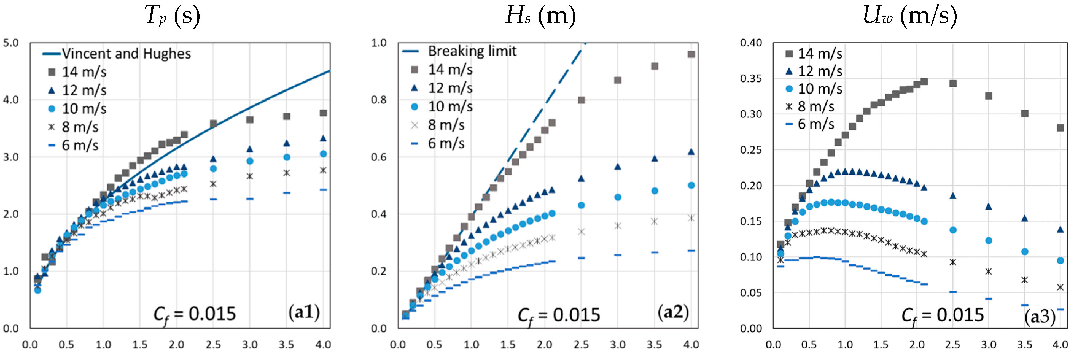
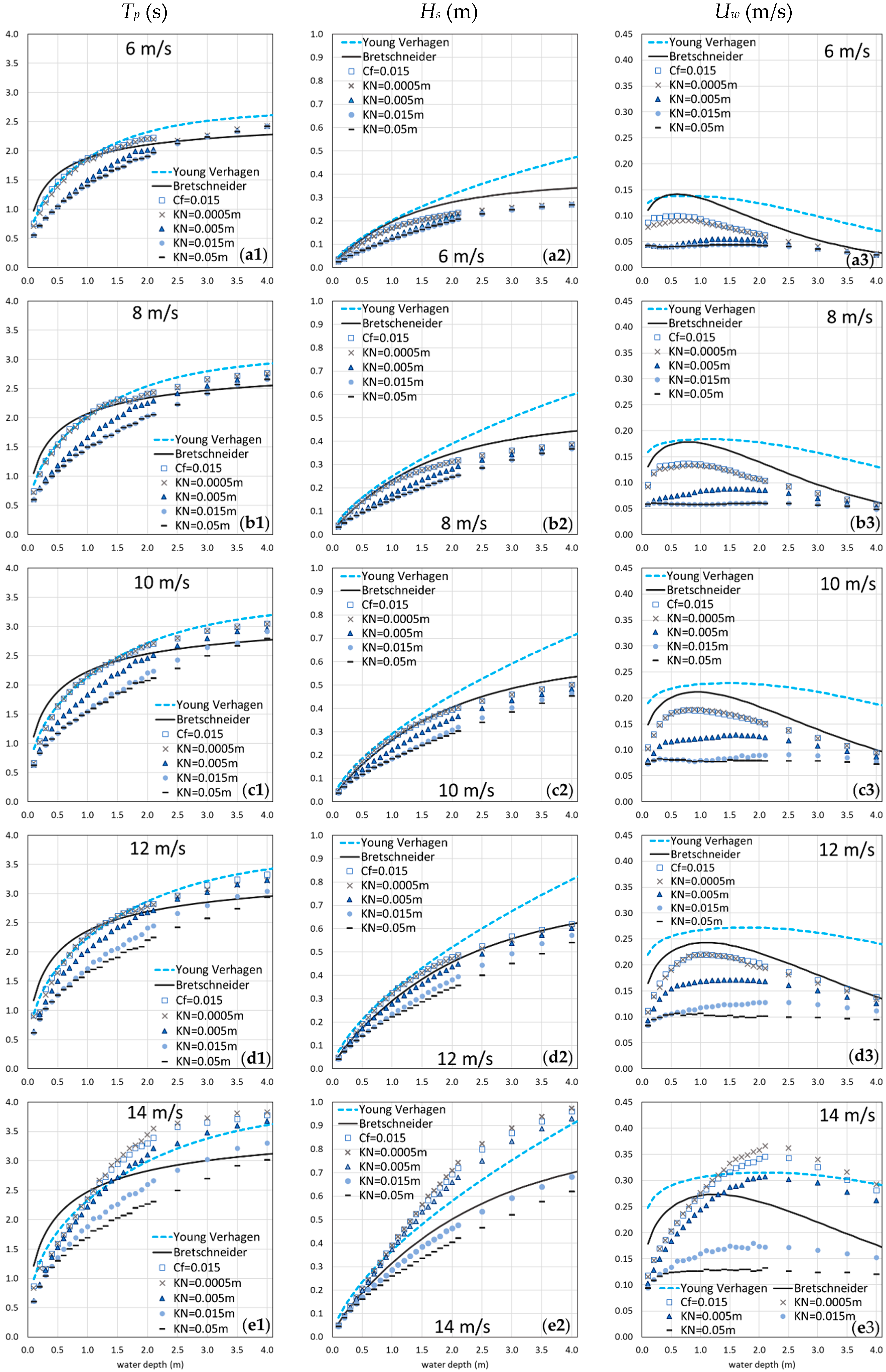
4.1. Main Characteristics of the Wave Field

For a better understanding of the results, a discussion based on the wave characteristics and not the related dimensionless variables defined in Section 2 is preferred. The distributions at varying depths of the main parameters of the wave field generated for different values of wind speed and bed roughness are firstly presented. Specifically, in Figure 1 the wave peak period T_p, the significant wave height H_s, and the root mean square value of the maxima of the orbital velocity near the bottom U_w are depicted.

The wave parameters correspond to a fully developed sea condition achieved with the perfect balance between the energy transferred by wind to the water surface and the dissipations due to the source terms related to interaction with bottom. Each graph compares the trend of the parameters obtained with the five different wind speeds, for the given class of bottom roughness among the five evaluated conditions, distinguishing between the Collins and Madsen approaches to compute the spectral friction dissipations. The crucial role played by friction is highlighted on observing the graphs arranged from top to bottom in an increasing order of the K_N value, which involves the progressive reduction of all the wave field characteristics.

In particular, the results of Figure 1(a1–e1) are in agreement with the Vincent and Hughes theory [34], that establishes an upper limit for the peak period of wind waves generated on shallow depths, here coinciding with the continuous line obtained by means of the Equation (9). This constraint is very significant for depths less than 2 m, typical of tidal flats and mudflats, and causes a variability of the period that cannot therefore be considered constant [27].

Moreover, as can be seen, the increase in the bottom roughness significantly reduces the value of the period that moves away from the upper limit of Vincent and Hughes [34] and becomes almost independent from the wind speed. In this sense, the bottom friction dissipation becomes one of the dominant factors of the generation process.

This outcome is even more evident when observing the trend of the wave heights reported in Figure 1(a2–e2). The dashed line represents the limit given by the depth-induced wave breaking, which is reached on very small depths of less than 50 cm. Only the wave motion generated by a wind of 14 m/s on a very smooth flat bottom, can breaks on a depth of about 1.0–1.2 m, which corresponds to the mean depth of coastal lagoons like that of Marano and Grado or Venice [22,44]. With increasing bottom roughness, the plot exhibits a quasi-linear relationship between the wave height and the local water depth, as seen in Figure 1(d2–e2), which however is much lower than the breaking limit. This conclusion is in perfect agreement with the observations of Wells and Kemps [53] and Le Hir et al. [9], who stated that the reason for this saturation of the local wave height on flats can be looked for in bottom friction. Treating analytically the simplified case of a monochromatic wave propagating on a uniform slope, Le Hir et al. [9] have also deduced that the maximum wave height such a tidal flat can experience at a given water depth, is a function of the ratio between the friction factor and the bed slope. For large values of such parameter, that means high friction or gentle slope, dissipations become dominant.

Consistently with this achievement, examining the curves obtained in the present simulations with the stronger winds, the effects of the frictional dissipation are clearly detected, since the wave energy, and therefore the resulting wave height and the wave bottom orbital velocity are greatly reduced by higher bed roughness, attributable for example to bedforms. In this regard, it should be emphasized that, if the limitation on period and wave height growth was already observed and analytically defined, there are no similar considerations on the effects of frictional dissipation on the bottom orbital velocities. However, these velocities are decisive for sediment transport processes, since the wave bottom shear stresses depend on them according to a quadratic law.

As Figure 1(a3–e3) show, the most evident aspect is that on a smooth flat bed the bottom orbital velocity increases up to a peak value, reached at a water depth related to the wind speed, and then decreases for greater depths.

This is analogous to the description provided by Fagherazzi et al. [22] on the shear stress curve, computed for a characteristic wind speed of 8 m/s and a very small equivalent bed roughness of 5 × 10⁻⁷ m, related to a mean grain diameter of 20 µm. However, it is sufficient to have a weakly irregular bottom, with a more heterogeneous granulometry, meaning K_N is at least equal to a few millimeters, that the curves tend to flatten and follow an almost constant trend on the analyzed depths, especially for less intense winds.

To better understand the effect of bottom friction on wave motion, the same quantities described above are depicted in Figure 2, where each graph presents the results obtained with different values for bed roughness but the same wind speed. In particular, the comparison with the limits to wind growth given by Young and Verhagen [35] (the dashed line) and Bretschneider [33] (the continuous line) is reported.

As described in Section 2, Young and Verhagen [35] have refined the relationships provided by Bretschneider [33] on the basis of an extensive data set of wave parameters collected inside the shallow and quite uniform in-depth Lake George. In particular, they have found a significantly lower value for the peak period. Consistent with this outcome and recognized by observing the dotted line in Figure 2(a1–e1), is that on depths below 1.2 m a lower limit for the period is predicted and this limit is therefore respected by all points, regardless of the different conditions of roughness and wind speed.

The case is different for wave height: the upper limit of Bretschneider is more restrictive everywhere compared to that of Young and Verhagen, but it better interprets the distributions obtained with the simulations, especially concerning those performed with the Collins approach and Madsen formula with a K_N of 0.0005 m, whose results are almost overlapping.

This coincidence is explained computing the K_N equivalent value related to the Collins constant friction factor as a mean of the values obtained according to Equations (3) and (4) with the assumption of rough turbulent motion. As reported in

Table 2. Values of equivalent K_N in the simulations performed by applying Collins frictional law.

Simulation	W6Col	W8Col	W10Col	W12Col	W14Col
Equivalent KN (m)	0.0002	0.0004	0.0005	0.0007	0.0011

the equivalent K_N has an average value of 0.0006 m.

The wave heights generated by a wind speed of 14 m/s on a smooth and regular bottom (Figure 2(e2)) exceed both experimental curves. In fact, this is a fairly strong velocity that exits the range of data set used for determining the coefficients of the growth curves, at least from that declared by Young and Verhagen. At moderate winds and greater roughness there is an almost linear trend of the wave height with the depth [9,53].

The combination of wave height and period greatly amplifies the differences between the bottom orbital velocities resulting from the interaction with different bed roughness as explained above. These differences are very marked especially for depths less than 1.5 m, that are relevant to this work. In this sense, Bretschneider wave parameters provide a bell shape curve of U_w, as the friction factor and consequently the corresponding K_N value are assumed very small by hypothesis. Nevertheless, the scatter points determined taking into account a heterogeneous bottom, are arranged according to decidedly more flattened trends on much lower values.

Considering the quadratic dependence of the bottom shear stresses from U_w it becomes essential to verify the effects that these differences of behavior for different roughness heights have on the trend of τ_w and whether the bell shape curve is effectively maintained as suggested in literature [22,27,45] or not.

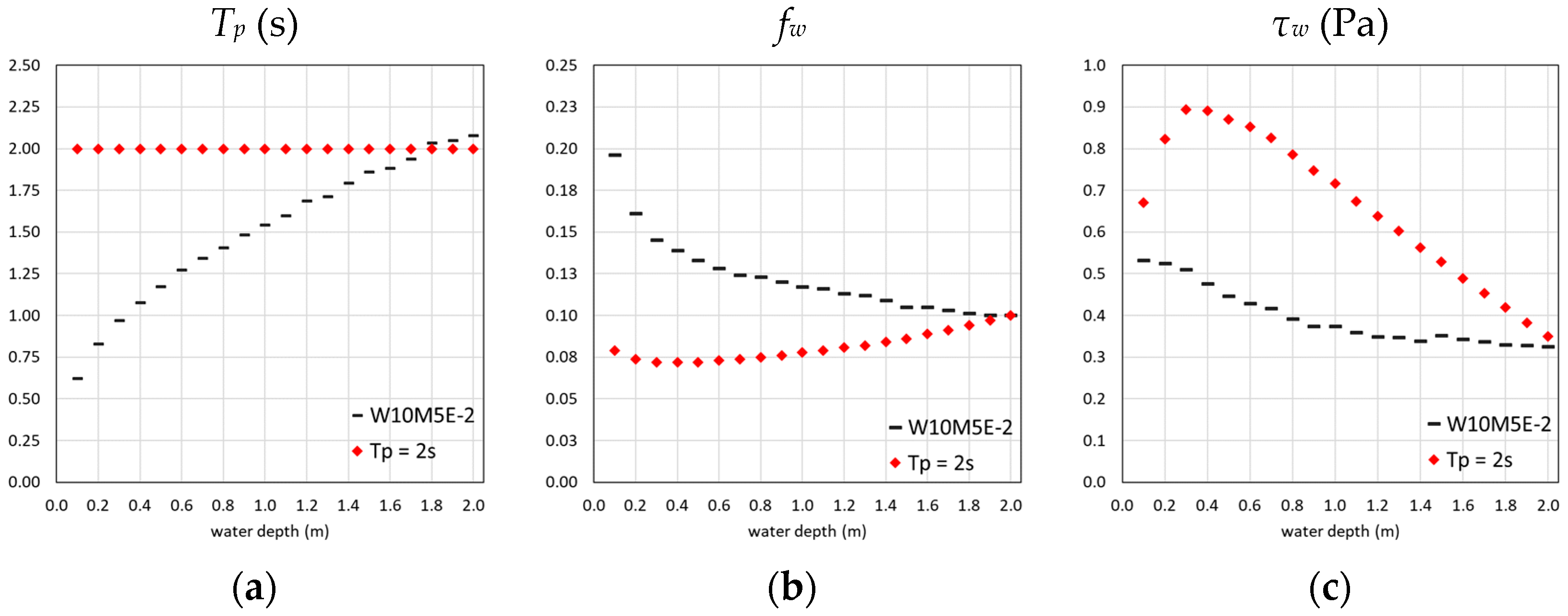
4.2. Analysis of the Bed Shear Stresses

In most areas in shallow seas or in estuarine and lagoon basins, the bed generally presents irregularities, both due to the non-uniform particle size composition and to current and wave-generated ripples, dunes and other bedforms [51,54]. On these non-flat beds, the total wave-induced bottom shear stress is composed of a skin-friction contribution acting on the sediment grain and which is responsible for resuspension mechanisms if the critical shear stress is exceeded, and a form-drag component which instead dissipates the energy of the current and the wave motion [26]. The expression for both these wave shear stress components is the same as suggested in Equation (13), what varies is the different value of the friction factor f_w and the associated bed roughness. In the first case, the Nikuradse roughness K_N can be evaluated as an expression of the median diameter if the bed is composed of coarse grains, while for fine cohesive grains or mud-beds, K_N can be set to the height of protrusions as an approximation [54]. In the case of the form-drag shear stress, the friction factor and consequently the bed roughness have to take into account the larger features on the bed and hence the size of the ripple or the generic bedform, as pointed out above in Section 3.

This section focuses on the skin friction bed shear stress dependence on water depth, as this is relevant in sediment dynamics. The main results are displayed in Figure 3.

The friction factor entering in Equation (13) has been computed by adopting the Soulsby formulation as given by Equation (4). This is an extensive choice taken by many authors [13,22,27,45,46,47] and it presupposes that a rough turbulent motion is realized near the bed. Only for a few cases f_w is assumed constant [21] and equal to a calibrated parameter. In the present study a value of 0.005 m of the Nikuradse equivalent roughness has been taken to define the z₀ value entering in the skin friction bottom shear stress, representing a generic condition of a non-flat bed with uneven granulometry and coexistence of sand and mud, as typically happens in lagoon and estuarine environments [44].

The wave parameters and specifically the horizontal orbital excursion A, have been taken from all the performed simulations to better highlight the role played by the bed roughness and the consequent bottom friction dissipations.

The variable distribution of the friction factor at different water depths as depicted in Figure 3(a1–e1) is quite evident. If the wind is strong enough, which means speed of at least 12 m/s, f_w is fairly constant on depths higher than 1.5 m, regardless of the roughness used to compute spectral friction dissipations, but remaining in any case greater than the friction factor f_wC assumed by Collins.

Otherwise on shallower depths, which are representative of generic tidal flats, the spread is remarkable in relation to both wind and roughness. In particular, the wave field generated by moderate or low winds gives much higher values of f_w depending on the bottom conformation, with important effects on the wave shear stress trend. The comparison between the bottom orbital velocity curves depicted in Figure 1(a3–e3) with the corresponding bed shear stress curves in Figure 3(a2–e2) points out that the increase in friction factor means the loss of the bell shape curve, the bottom shear stress tending to descend monotonically with the water depth. Moreover, if a K_N value of a few cm is assigned [13] and hence the bottom is more dissipative, the bed shear stress values obtained for different wind conditions are very close to each other.

This statement is coherent with the observed trends in bed shear stresses over a mudflat, as reported by Mariotti et al. [27], who have not found in either the measured or simulated data an obvious dependence on water depth as happens for wave heights and periods related to a wind speed range of 5–10 m/s. The functional relationship between bed shear stress and depth previously derived by Fagherazzi et al. [22] predicts that the bed shear stress initially increases and then decreases with deeper waters. Mariotti et al. [27] attributed the divergence with observed trends to the role of a variable wave period, that has been instead assumed as constant in depth and equal to 2 s by Fagherazzi et al. [22].

To prove this link, Mariotti et al. [27] explored the relationship between bottom shear stress and depth by means of SWAN model but keeping the Collins approach to compute spectral friction dissipation. This assumption, however, neglects the variability of the period in the friction dissipations, f_wC being a constant, and moreover implies that the bed is perfectly smooth for the wave field predicted on this range of water depths, as explained in Section 4.1. The variability of the wave period for wind waves generated on finite depths is a key condition in understanding the behavior of the bed shear stresses, both for those related to energy dissipations and for those related to the sediment grains as the skin-friction component. This work emphasizes this important result, that has never been investigated previously. Figure 4 clarifies this concept.

The graphs compare two conditions: on the one hand the results given by the simulation performed with the major bed dissipative configuration (Madsen approach and a K_N value of 0.05 m) and a wind speed of 10 m/s, considered as dominant for morphological evolution of estuarine and tidal environments by many authors [13,15,44]; on the other hand the same variables, f_w and τ_w respectively, are computed by recalculating the bottom orbital velocities assuming a fixed peak period of 2 s and the wave heights obtained from the previous simulation. The comparison effectively shows that, if the wave period is kept constant, the bell shape curve of the bed shear stress is found again but it is only fictitious. Furthermore, if the wave period changes with depth, so does the friction factor and hence it should not be considered constant as in the Collins approach.

Another reason, besides the latter, that leads to discouraging the Collins formula for numerical applications in shallow and confined estuarine and tidal environments, is that it provides much higher bottom shear stresses than those obtained with the Madsen approach. This happens because the equivalent roughness, under the hypothesis of rough turbulent motion near the bed, is very low like the friction factor, and therefore it induces a weak energy dissipation. Consequently the bottom orbital velocities are significantly higher and the shear stresses also increase although f_w remains bounded.

This outcome becomes clearer from a comparison with a critical shear stress, reported in Figure 3(a3–e3). The dotted line refers to a value of 0.7 Pa, representative for the erosion of cohesive sediments as results in the North Adriatic Sea lagoons and estuarine contexts [13,22,44,55,56]. For wind speeds greater than 8 m/s, the two curves of the bottom shear stress deriving from the simulations that adopt respectively Collins and Madsen formula with K_N equal to 0.0005 m, would almost always give an erosion condition on all the depths up to 2 m, without considering the further contribution of the currents. If a much lower critical shear stress would be considered, about 0.1–0.15 Pa as reported from other sites [19,27,46,47] this effect would also be greatly amplified for very low wind speeds.

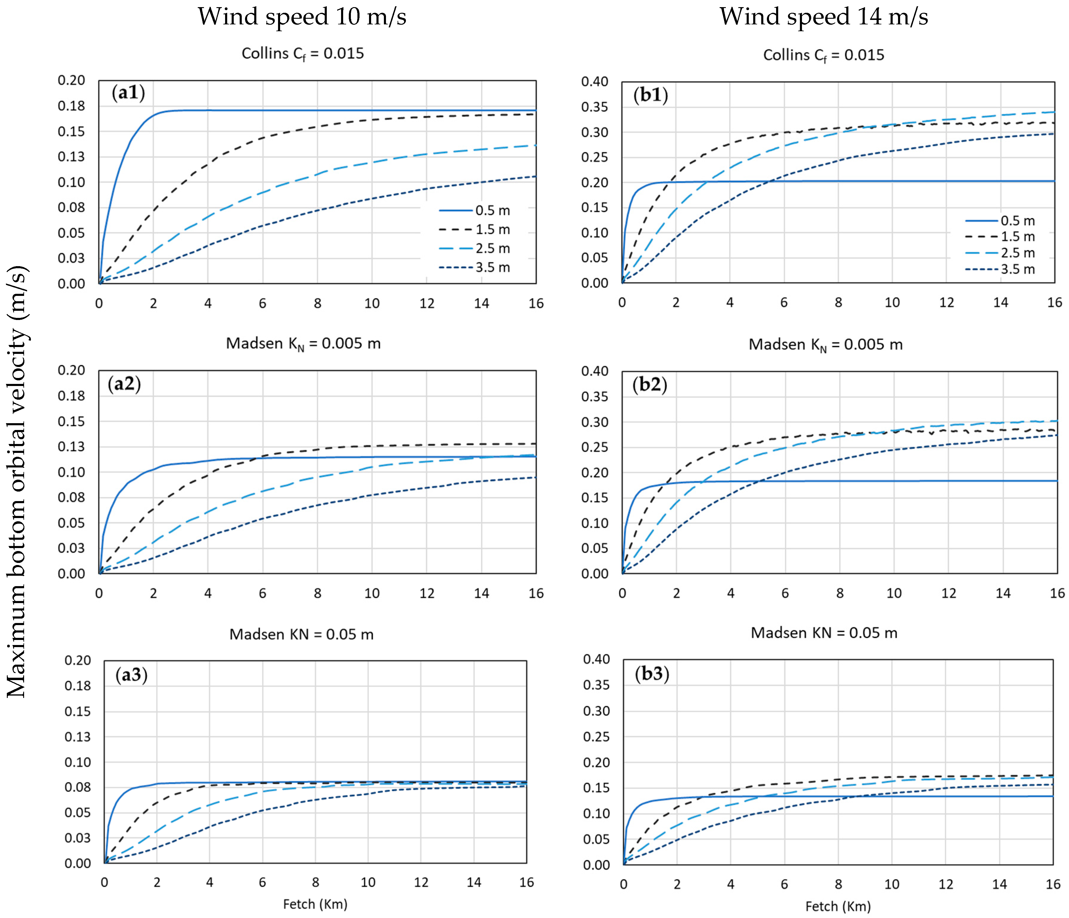
4.3. Considerations on the Fetch Dependence of the Bed Shear Stresses

The results presented and discussed in the previous sections refer to a fully developed sea condition for the assigned conditions of wind speed, fetch and depth, and hence the dependence on the fetch has not yet been considered. However, it is possible to make some considerations about this.

Mariotti et al. [27] showed that for small water depths lesser than 1 m and strong wind speeds of about 15 m/s, the wave bottom shear stress has almost no dependence on fetch, while the contrary happens on larger water depth, where the dependence on fetch becomes relevant. Moreover, for fixed wind speed and water depth, τ_w monotonically increases with fetch, tending asymptotically to the maximum value which can be obtained for a fully developed state. In shallower waters, this upper limit is reached faster compared to relatively deep depths. They also stated that the large differences between the values of the bed shear stress related to different depth at the same wind speed, occur for fetches of about 2.5–20 km, which are the typical extension of tidal flats. These conclusions are correct in relation to the Collins spectral bottom friction dissipation imposed by Mariotti et al. [27], but for this reason they can be improved.

All the main characteristics of the wave motion generated on finite depths are strongly influenced by the frictional characteristics of the bottom, which can be very heterogeneous in transitional contexts as previously underlined. In particular, the bottom orbital velocity, from which the shear stress directly derives, tends to a quite uniform distribution with the increase in the bottom roughness, regardless of wind speed. In line with this result, it is quite obvious to imagine that similar effects can be found for the dependence on the fetch.

With the aim to complete the present study, a comparison between the bottom orbital velocities obtained as a function of the fetch is made, choosing some depths and bottom roughness configurations. Wind speeds of 10 m/s and 14 m/s are taken as representative for this purpose, as in Mariotti et al. [27].

Figure 5 shows effectively that the bottom orbital velocity tends to an upper value related to wind, depth and fetch conditions, as usually happens in the generation process on finite depths. This maximum limit is reached faster on shallower depths and moderate winds (10 m/s), but in the presence of higher conditions of bottom roughness it is reached even on shorter distances.

These conditions are representative of lagoon environments, whereas many tidal flats have less than 2 m depth. In those cases, the fully developed state can already be achieved with fetch on the order of a few km, especially in presence of moderate winds, which are strong enough to make resuspension of sediments in any case. This outcome is in agreement with the results of Petti et al. [44] who found that inside a lagoon basin even shorter free sea distances can give comparable wave motion characteristics independently of the wind direction that optimizes the fetch.

These considerations complete and strengthen the role of the bottom roughness length and friction dissipations for wind waves locally generated on shallow basins.

5. Conclusions

The wind wave field generated on finite depths, inside confined basins like estuarine environments and shallow lagoons, has been investigated by means the spectral model SWAN, for different patterns of wind speed and bottom composition, the latter synthetized by a specific value of the Nikuradse parameter.

The main characteristics of the wave motion have been compared with experimental growth curves provided by many authors, who have estimated the upper values that the peak period and the significant wave height could reach for assigned water depth, wind speed and fetch. These limits have been determined adopting a low friction factor, generally representative of very smooth and flat beds. However, the comparison with the obtained numerical results highlighted that, on shallow depth, the friction factor depends strongly by the wave period and the roughness entity, revealing itself as a key parameter to understanding the behavior of the bottom shear stress caused by the interaction with the bed irregularities.

In several applications the loss of energy caused by the bottom friction is computed by adopting the drag-based formula of Collins [28], which is easier to implement, and it does not involve calibration parameters assuming a constant f_w. Differently, Madsen et al. [30] have suggested an approach linked to a particular value of the roughness height and, in this sense, to the bottom conformation. The performed simulations showed that this approach is more suitable to be adopted in applications in coastal and transitional environment, where for the simultaneous presence of waves and currents and their non-linear interactions, the sea bed is generally characterized by the coexistence of sand and mud and the presence of ripples, dunes, or even vegetation.

The results obtained from the two different spectral formulations effectively show that the Collins approach corresponds to the assumption of a very smooth and regular bottom, which is not however consistent with the real morphological patterns of the environments to which the application refers. In particular, even a small increase in the bottom roughness can significantly reduce all the wave characteristics, pointing out that friction dissipation is one of the dominant factors of the generation process and for this reason it must be correctly represented.

In this sense, the present study has showed that the bottom orbital velocity and therefore the related bottom shear stress are strongly affected by dissipation effects through their dependence on the wave period and the friction factor. A comparative analysis of the relationship of these quantities with depth has been made according to different bed roughness values. In the presence of an irregular bed morphology and composition, which means K_N equal at least to a few millimeters, the distribution of the wave bottom shear stress on the water depth loses the non-monotonic trend so far suggested by some authors, tending instead to decrease on the overall bathymetries and toward much lower values related to a fully developed state condition. This latter state is consequently reached on much shorter distances, as usually happens in tidal and confined contexts.

For these reasons, the present work provides a fuller interpretation of the relationship between τ_w and the water depth accounting for wave period and bottom roughness effects, and it supplies useful suggestions for numerical applications in shallow and confined estuarine and tidal environments.

References

1. Galloway, W.E. Process framework for describing the morphologic and stratigraphic evolution of deltaic depositional systems. In Deltas: Models for Exploration; Broussard, M.L., Ed.; Houston Geological Society: Houston, TX, USA, 1975; pp. 87–98. [Google Scholar]
2. Bhattacharya, J.P. Deltas. In Facies Models Revisited; Posamentier Henry, W., Walker Roger, G., Eds.; SEPM (Society for Sedimentary Geology) Special Publication: Broken Arrow, OK, USA, 2006; Volume 84, pp. 237–292. ISBN 9781565761216. [Google Scholar] [CrossRef]
3. Wright, L.D.; Coleman, J.M. Variations in morphology of major river deltas as functions of ocean wave and river discharge regimes. AAPG Bull. 1973, 57, 370–398. [Google Scholar]
4. Bhattacharya, J.P.; Giosan, L. Wave-influenced deltas: Geomorphological implications for facies reconstruction. Sedimentology 2003, 50, 187–210. [Google Scholar] [CrossRef]
5. Ashton, A.D.; Giosan, L. Wave angle control of delta evolution. Geophys. Res. Lett. 2011, 38, L13405. [Google Scholar] [CrossRef]
6. Friedrichs, C.L. Tidal flat morphodynamics: A synthesis. In Treatise on Estuarine and Coastal Science; Estuarine and Coastal Geology and Geomorphology; Hansom, J.D., Fleming, B.W., Eds.; Elsevier: Amsterdam, The Netherlands, 2011; Volume 3, pp. 137–170. [Google Scholar]
7. Friedrichs, C.T.; Perry, J.E. Tidal Salt Marsh Morphodynamics: A Synthesis. J. Coast. Res. 2001, SI 27, 7–37. [Google Scholar] [CrossRef]
8. Allen, J.R.L.; Duffy, M.J. Medium-term sedimentation on high intertidal mudflats and salt marshes in the Severn Estuary, SW Britain: The role of wind and tide. Mar. Geol. 1998, 150, 1–27. [Google Scholar] [CrossRef]
9. Le Hir, P.; Roberts, W.; Cazaillet, O.; Christie, M.; Bassoullet, P.; Bacher, C. Characterization of intertidal flat hydrodynamics. Cont. Shelf Res. 2000, 20, 1433–1459. [Google Scholar] [CrossRef] [Green Version]
10. Roberts, W.; Le Hir, P.; Whitehouse, R.J.S. Investigation using simple mathematical models of the effect of tidal currents and waves on the profile shape of intertidal mudflats. Cont. Shelf Res. 2000, 20, 1079–1097. [Google Scholar] [CrossRef]
11. Lanzoni, S.; Seminara, G. Long term evolution and morphodynamic equilibrium of tidal channels. J. Geophs. Res. 2002, 107 C1, 1–13. [Google Scholar] [CrossRef]
12. Cappucci, S.; Amos, C.L.; Hosoe, T.; Umgiesser, G. SLIM: A numerical model to evaluate the factors controlling the evolution of intertidal mudflats in Venice Lagoon, Italy. J. Mar. Syst. 2004, 51, 257–280. [Google Scholar] [CrossRef]
13. Umgiesser, G.; Sclavo, M.; Carniel, S.; Bergamasco, A. Exploring the bottom shear stress variability in the Venice Lagoon. J. Mar. Syst. 2004, 51, 161–178. [Google Scholar] [CrossRef]
14. Fagherazzi, S.; Palermo, C.; Rulli, M.C.; Carniello, L.; Defina, A. Wind waves in shallow microtidal basins and the dynamic equilibrium of tidal flats. J. Geophys. Res. 2007, 112, F02024. [Google Scholar] [CrossRef]
15. Fagherazzi, S.; Wiberg, P.L. Importance of wind conditions, fetch, and water levels on wave-generated shear stresses in shallow intertidal basins. J. Geophys. Res. 2009, 114, F03022. [Google Scholar] [CrossRef]
16. Callaghan, D.P.; Bouma, T.J.; Klaassen, P.; van der Wal, D.; Stive, M.J.F.; Herman, P.M.J. Hydrodynamic forcing on salt-marsh development: Distinguishing the relative importance of waves and tidal flows. Estuar. Coast. Shelf Sci. 2010, 89, 73–88. [Google Scholar] [CrossRef]
17. Green, M.O. Very small waves and associated sediment resuspension on an estuarine intertidal flat. Estuar. Coast. Shelf Sci. 2011, 93, 449–459. [Google Scholar] [CrossRef]
18. Carniello, L.; Defina, A.; D’Alpaos, L. Modeling sand-mud transport induced by tidal currents and wind waves in shallow microtidal basins: Application to the Venice Lagoon (Italy). Estuar. Coast. Shelf Sci. 2012, 102, 105–115. [Google Scholar] [CrossRef]
19. Shi, B.W.; Yang, S.L.; Wang, Y.P.; Bouma, T.J.; Zhu, Q. Relating accretion and erosion at an exposed tidal wetland to the bottom shear stress of combined current–wave action. Geomorphology 2012, 138, 380–389. [Google Scholar] [CrossRef]
20. Zhou, Z.; Coco, G.; van der Wegen, M.; Gong, Z.; Zhang, C.; Townend, I. Modeling sorting dynamics of cohesive and non-cohesive sediments on intertidal flats under the effect of tides and wind waves. Cont. Shelf Res. 2015, 104, 76–91. [Google Scholar] [CrossRef]
21. Green, M.O.; Coco, G. Review of wave-driven sediment resuspension and transport in estuaries. Rev. Geophys. 2014, 52, 77–117. [Google Scholar] [CrossRef] [Green Version]
22. Fagherazzi, S.; Carniello, L.; D’Alpaos, L.; Defina, A. Critical bifurcation of shallow microtidal landforms in tidal flats and salt marshes. Proc. Natl. Acad. Sci. USA 2006, 103, 8337–8341. [Google Scholar] [CrossRef] [PubMed] [Green Version]
23. Fredsøe, J.; Deigaard, R. Mechanics of Coastal Sediment Transport; Advanced Series on Ocean Engineering; World Scientific: Singapore, 1992; Volume 3, 369p. [Google Scholar]
24. Van Rijn, L.C. Principles of Sediment Transport in Rivers, Estuaries and Coastal Seas; Aqua Publications: Amsterdam, The Netherlands, 1993; 715p. [Google Scholar]
25. Madsen, O.S. Spectral Wave-Current Bottom Boundary Layer Flows. Coast. Eng. 1994, 29, 384–398. [Google Scholar] [CrossRef]
26. Soulsby, R.L. Dynamics of Marine Sands: A Manual for Practical Applications; Thomas Telford Publications: London, UK, 1997; 249p. [Google Scholar]
27. Mariotti, G.; Fagherazzi, S. Wind waves on a mudflat: The influence of fetch and depth on bed shear stresses. Cont. Shelf Res. 2013, 60, S99–S110. [Google Scholar] [CrossRef]
28. Collins, J.I. Prediction of shallow water spectra. J. Geophys. Res. 1972, 77, 2693–2707. [Google Scholar] [CrossRef]
29. Hsiao, S.V.; Shemdin, O.H. Bottom Dissipation in Finite-Depth Water Waves. Coast. Eng. 1978, 24, 434–448. [Google Scholar] [CrossRef]
30. Madsen, O.S.; Poon, Y.-K.; Graber, H.C. Spectral wave attenuation by bottom friction: Theory. In Proceedings of the 21th International Conference Coastal Engineering, Costa del Sol-Malaga, Spain, 20–25 June 1988; pp. 492–504. [Google Scholar]
31. Bretschneider, C.L.; Reid, R.O. Change in Wave Height Due to Bottom Friction, Percolation and Refraction; Beach Erosion Board Engineer Research and Development Center (U.S.): Boston, MA, USA, 1954. [Google Scholar]
32. CERC (U.S. Army Coastal Engineering Research Center). Shore Protection Manual; U.S. Army Coastal Engineering Research Center: Washington, DC, USA, 1973. [Google Scholar]
33. CERC (U.S. Army Coastal Engineering Research Center). Shore Protection Manual; U.S. Army Coastal Engineering Research Center: Washington, DC, USA, 1984. [Google Scholar]
34. Vincent, C.L.; Hughes, S.A. Wind Wave Growth in Shallow Water. J. Waterw. Port Coast. Ocean Eng. 1985, 111, 765–770. [Google Scholar] [CrossRef]
35. Young, I.R.; Verhagen, L.A. The growth of fetch limited waves in water of finite depth. 1. Total energy and peak frequency. Coast. Eng. 1996, 29, 47–78. [Google Scholar] [CrossRef]
36. Hasselmann, K.; Collins, J.I. Spectral dissipation of finite-depth gravity waves due to turbulent bottom friction. J. Mar. Res. 1968, 26, 1–12. [Google Scholar]
37. Zijlema, M.; van Vledder, G.P.; Holthuijsen, L.H. Bottom friction and wind drag for wave models. Coast. Eng. 2012, 65, 19–26. [Google Scholar] [CrossRef]
38. Pascolo, S.; Petti, M.; Bosa, S. Wave–Current Interaction: A 2DH Model for Turbulent Jet and Bottom-Friction Dissipation. Water 2018, 10, 392. [Google Scholar] [CrossRef]
39. Booij, N.; Ris, R.C.; Holthuijsen, L.H. A third-generation wave model for coastal regions, Part I, Model description and validation. J. Geophys. Res. 1999, 104, 7649–7666. [Google Scholar] [CrossRef]
40. Jonsson, I.G. Wave Boundary Layers and Friction Factors. In Proceedings of the Tenth International Conference on Coastal Engineering, Tokyo, Japan, 5–8 September 1966; pp. 127–148. [Google Scholar] [CrossRef]
41. Kamphuis, W. Friction Factor under Oscillatory Waves. J. Waterw. Harb. Coast. Eng. Div. 1975, 101, 135–144. [Google Scholar]
42. Myrhaug, D. A rational approach to wave friction coefficients for rough, smooth and transitional turbulent flow. Coast. Eng. 1989, 13, 11–21. [Google Scholar] [CrossRef]
43. Ijima, T.; Tang, F.L.W. Numerical Calculation of Wind Waves in Shallow Water. Coast. Eng. 1966, 38–49. [Google Scholar] [CrossRef]
44. Petti, M.; Bosa, S.; Pascolo, S. Lagoon Sediment Dynamics: A Coupled Model to Study a Medium-Term Silting of Tidal Channels. Water 2018, 10, 569. [Google Scholar] [CrossRef]
45. Carniello, L.; Defina, A.; D’Alpaos, L. Morphological evolution of the Venice lagoon: Evidence from the past and trend for the future. J. Geophys. Res. 2009, 114, F04002. [Google Scholar] [CrossRef]
46. Zhu, Q.; van Prooijen, B.C.; Wang, Z.B.; Yang, S.L. Bed-level changes on intertidal wetland in response to waves and tides: A case study from the Yangtze River Delta. Mar. Geol. 2017, 385, 160–172. [Google Scholar] [CrossRef]
47. Shi, B.; Cooper, J.R.; Pratolongo, P.D.; Gao, S.; Bouma, T.J.; Li, G.; Li, C.; Yang, S.L.; Wang, Y.P. Erosion and accretion on a mudflat: The importance of very shallow-water effects. J. Geophys. Res. Oceans 2017, 122, 9476–9499. [Google Scholar] [CrossRef]
48. Cavaleri, L.; Rizzoli, P.M. Wind wave prediction in shallow water: Theory and applications. J. Geophys. Res. 1981, 86, 10961–10973. [Google Scholar] [CrossRef]
49. Janssen, P.A.E.M. Quasi-linear theory of wind-wave generation applied to wave forecasting. J. Phys. Oceanogr. 1991, 21, 1631–1642. [Google Scholar] [CrossRef]
50. Holthuijsen, L.H. Waves in Oceanic and Coastal Waters; Cambridge University Press: Cambridge, UK, 2007. [Google Scholar]
51. Nielsen, P. Coastal and Estuarine Processes; Advanced Series on Ocean Engineering; World Scientific: Singapore, 2009; Volume 29, p. 345. [Google Scholar]
52. Chirol, C.; Amos, C.L.; Kassem, H.; Lefebvre, A.; Umgiesser, G.; Cucco, A. The Influence of Bed Roughness on Turbulence: Cabras Lagoon, Sardinia, Italy. J. Mar. Sci. Eng. 2015, 3, 935–956. [Google Scholar] [CrossRef]
53. Wells, J.T.; Kemp, G.P. Interaction of surface waves and cohesive sediments: Field observations and geologic significance. In Estuarine Cohesive Sediment Dynamics; Lecture Notes on Coastal and Estuarine Studies N314; Mehta, A.J., Ed.; Springer: Berlin, Germany, 1986; pp. 43–65. [Google Scholar]
54. Whitehouse, R.J.S.; Soulsby, R.L.; Roberts, W.; Mitchener, H.J. Dynamics of Estuarine Muds; Technical Report; Thomas Telford: London, UK, 2000. [Google Scholar]
55. Amos, C.L.; Bergamasco, A.; Umgiesser, G.; Cappucci, S.; Cloutier, D.; Denat, L.; Flindt, M.; Bonardi, M.; Cristante, S. The stability of tidal flats in Venice Lagoon—The results of in-situ measurements using two benthic, annular flumes. J. Mar. Syst. 2004, 51, 211–241. [Google Scholar] [CrossRef]
56. Bosa, S.; Petti, M.; Pascolo, S. Numerical Modelling of Cohesive Bank Migration. Water 2018, 10, 961. [Google Scholar] [CrossRef]
Figure 1. Distribution at varying water depths of the wave field for different KN values: (a1e1) the peak period, (a2e2) the significant wave height, and (a3e3) the root mean square value of the maxima of the orbital velocity near the bottom.
Water 10 01348 g001aWater 10 01348 g001b
Figure 2. Distribution at varying water depths of the wave field for increasing wind speeds: (a1e1) the peak period, (a2e2) the significant wave height, and (a3e3) the root mean square value of the maxima of the orbital velocity near the bottom.
Water 10 01348 g002
Figure 3. Distribution of: (a1e1) the wave friction factor; (a2e2) and (a3e3) the bed shear stress. The dashed line refers to the Young and Verhagen growth curve, the continuous line to Bretschneider approach. fw Collins is the constant friction factor assumed by Collins. Tcrit is a critical shear stress.
Water 10 01348 g003aWater 10 01348 g003b
Figure 4. Comparison between the results given by the simulation W10M5E-2 with the same ones obtained keeping the peak period constant, in terms of: (a) Tp; (b) fw and (c) τw.
Water 10 01348 g004
Figure 5. Bottom orbital velocity as a function of fetch for a wind speed of: (a1a3) 10 m/s and (b1b3) 14 m/s, and increasing bottom roughness from top to bottom.
Water 10 01348 g005