Case Study of Heat Transfer during Artificial Ground Freezing with Groundwater Flow

Abstract

For the artificial ground freezing (AGF) projects in highly permeable formations, the effect of groundwater flow cannot be neglected. Based on the heat transfer and seepage theory in porous media with the finite element method, a fully coupled numerical model was established to simulate the changes of temperature field and groundwater flow field. Firstly, based on the classic analytical solution for the frozen temperature field, the model’s ability to solve phase change problems has been validated. In order to analyze the influences of different parameters on the closure time of the freezing wall, we performed the sensitivity analysis for three parameters of this numerical model. The analysis showed that, besides the head difference, the thermal conductivity of soil grain and pipe spacing are also the key factors that control the closure time of the frozen wall. Finally, a strengthening project of a metro tunnel with AGF method in South China was chosen as a field example. With the finite element software COMSOL Multiphysics^® (Stockholm, Sweden), a three-dimensional (3D) numerical model was set up to simulate the change of frozen temperature field and groundwater flow field in the project area as well as the freezing process within 50 days. The simulation results show that the freezing wall appears in an asymmetrical shape with horizontal groundwater flow normal to the axial of the tunnel. Along the groundwater flow direction, freezing wall forms slowly and on the upstream side the thickness of the frozen wall is thinner than that on the downstream side. The actual pipe spacing has an important influence on the temperature field and closure time of the frozen wall. The larger the actual pipe spacing is, the slower the closing process will be. Besides this, the calculation for the average temperature of freezing body (not yet in the form of a wall) shows that the average temperature change of the freezing body coincides with that of the main frozen pipes with the same trend.

1. Introduction

With its good water barrier and non-pollution characteristics, the artificial ground freezing (AGF) method is widespread in environmental engineering (e.g., excavation of pollutants) [1,2], mining engineering (e.g., mine shafts construction), and especially in underground engineering (e.g., subsea tunnel and urban subway construction) [3,4,5,6]. The basic principle of this method is to circulate a fluid refrigerant (ca. −30 °C) or liquid nitrogen (ca. −196 °C) through a pre-buried pipe network in the subsurface in order to form a freezing wall for strengthening construction or blocking groundwater flow.

Since its first application in Germany in 1887, the AGF method has been considerably developed in theory and practice. Especially in the conventional groundwater environment, for example, in freshwater and low flow rate conditions, this technology has been successfully applied in a large number of projects and it tends to be mature [7,8,9,10]. However, when this method is implemented under some special groundwater conditions, such as high groundwater flow velocity area, seawater invasion area, or groundwater heavily polluted area, the freezing effect will be affected by groundwater flow velocity, salt content, and different types of pollutants [11,12,13,14,15]. For instance, in the frozen wall project of the Fukushima Power Plant, the “Ice wall” failed to prevent groundwater infiltration. The most likely cause was the complex hydrological environment and the high concentration of radioactive toxic water [1]. This will bring new challenges to the typical application of the AGF method. In this paper, we mainly focus on the effect of flow velocity on the freezing effect from the perspective of groundwater flow.

During the development of freezing walls, groundwater flow and formation temperature distribution will interact with each other [11,16,17,18,19,20,21,22]. On the one hand, groundwater flow will take away the heat (coldness) around the freezing columns and slow down the cooling process of the formation. On the other hand, with the lowering of the formation temperature, the groundwater flow process will also be impacted. After the formation temperature reaches freezing point, an ice-water phase transition will occur in the pores, which will result in the formation of ice. Thereby, this will cause changes in the physical properties of the soil, such as permeability, density, thermal conductivity, and strength. The higher the flow velocity is, the stronger that the interaction will be. As the flow velocity increases, the heat transferred by the groundwater flow gradually replaces the heat extracted by the freezing pipes, slowing down the growth of the freezing columns around individual freezing pipes. This is a potential challenge for the AGF method.

In the past, many researchers have carried out research on the effect of groundwater flow on AGF method. First, some scholars have put forward corresponding numerical models from the viewpoint of heat-fluid coupling. Harlan (1973) [23] presented a mathematical model that coupled heat and fluid flow based on analogy and applied to the analysis of heat-fluid phenomena in partially frozen soil. Due to the lack of reliable data, quantitative comparisons of observed and simulated profile responses were not made. Using a finite element scheme, Guymon and Luthin (1974) [24] developed a one-dimensional a coupled model for heat and moisture based on the Richards equation and the heat conduction equation, including convective components, and applied this to analyze moisture movement and storage in Arctic soils. He pointed out that the feasibility of the model depends primarily on the assumption of equations and the computation costs. Hansson et al. (2004) [25] presented a new method that accounts for phase change in a fully implicit numerical model. This model was evaluated by comparing predictions with data from laboratory columns freezing experiments and applied this to simulate hypothetical road problems involving simultaneous heat transport and water flow. Based on some parametric assumptions, McKenzie et al. (2007) [26] simulated groundwater flow with energy transport numerically by modifying the SUTRA computer code and applied this to freezing processes in peat bogs. The model was validated by the analytical solution from Lunardini (1985) without an advection term [27]. Kurylyk et al. (2014) [28] reanalyzed this analytical solution and compared the results between the numerical solution and the Lunardini analytical solution with advection term. In the study of Scheidegger et al. (2017) [29], the development of permafrost was simulated with a two-dimensional (2D) thermo-hydro (TH) model using COMSOL software and this model was validated by this analytical solution. Tan et al. (2011) [30] established a TH coupling model based on the theories of continuum mechanics, thermodynamics, and segregation potential. The model considered the Soret effect, as well as the influence of segregation potential on groundwater flow velocity and water pressure distribution. This model has been verified by comparison with the well-known TH coupling laboratory test that was conducted by Mizoguchi (1990) [31].

Secondly, some scholars have focused on experimental studies of the AGF method combined with groundwater flow. Anton Sers (2009) [32] studied the growth of the freezing body with various groundwater flow velocities through a small-scale sandbox. Pimentel et al. (2012) [11] developed a large-scale physical experimental device for the AGF with high groundwater flow velocities and compared the experimental results of different experimental setups [33,34,35]. The results showed that, for the conditions of no groundwater flow or single freezing pipe, there were no substantial differences with respect to temperature change. But, with multiple pipes and high groundwater flow velocity, the discrepancies become larger as advection becomes more dominant in relation to heat conduction. Huang et al. (2012) [36] conducted a series of physical experiments and numerical simulations with controlled groundwater flow and boundary conditions. These results have shown that the growth of a freezing body is affected by groundwater flow.

It has been proven that the groundwater flow will affect the temperature distribution around the freezing pipes and further prevent the formation of the freezing wall. However, the quantification of the effect of groundwater flow velocity on the evolution of the freezing wall is still in dispute. Jessberger and Jagow (1996) [37] studied the effect of groundwater flow velocity on the AGF method with brine circulation and pointed to a flow velocity of 2 m/day as the critical limit. That is to say, the frozen body between the pipes will not close when the flow rate is more than 2 m/day. Besides this, Andersland and Ladanyi (2004) [38] claimed that, even with flow velocities between 1 and 2 m/day, no closure of the freezing body will occur. Other scholars have also given some different critical flow velocities [39,40].

In this work, we introduced the parameter of effective hydraulic conductivity and the saturation function of unfrozen water. Based on this parameter and function, we set up a fully coupled three-dimensional (3D) numerical model (COMSOL Multiphysics^® model with finite element) with groundwater flow field and frozen temperature field. This model is validated through the comparison of the results from numerical calculation and the analytical solution of the classic frozen problem from Lunardini [27] Its ability to solve the phase change problem is evaluated. With different numerical case studies, sensitivity analysis was performed for three parameters: the pipe spacing, thermal conductivity of soil grain and groundwater flow velocity (derived from hydraulic gradient or head difference). The corresponding influences of each parameter on the closure time of the freezing wall was analyzed. Finally, a strengthening project of a metro tunnel with AGF method in South China was chosen as an example for the field study. A numerical model was set up to simulate the artificial ground freezing process of this project. The regular pattern of frozen wall development was analyzed and the model was validated through the comparison of calculated and in-situ measured temperatures.

2. Methods

During the AGF process, thermal-hydraulic (TH) coupling is a key issue to be solved. As soil temperatures decrease below the freezing point, free water in the pores starts to freeze and the resulting ice crystals clog the original pore channels of groundwater flow. Simultaneously, due to the existence of convection, the change of the groundwater flow field will affect heat transfer in soil in return. In particular, the water-ice phase transition will lead to small changes in the physical properties of soil materials. The typical phase diagram of the freezing process is shown in Figure 1. In a saturated representative volume element (RVE), the pore space $\epsilon$ consists of ice, free water, and unfrozen film water, which are denoted by subscripts $i$, w, and $rs$, respectively. The saturation $S$, which describes the proportion of the volume occupied by the components in the pores, is introduced.

Based on the above coupling mechanism, we construct the mathematical model of this problem by establishing the governing equations of the groundwater flow field and the freezing temperature field, respectively. Through the multi-physics finite element software COMSOL Multiphysics^®, this problem can be numerically solved. Assumptions on this issue are required, as followed:

• the ice is immobile and the medium is non-deformable;
• the aquifer is fully saturated and its total porosity remains constant; and,
• the freezing point depression due to solute concentrations is negligible.

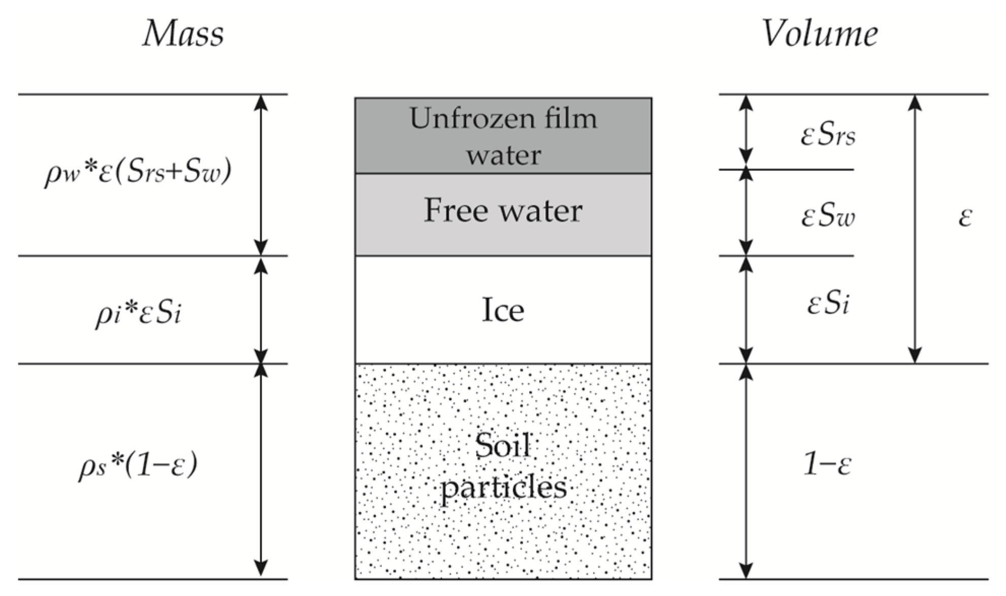
2.1. Water Mass Conservation Equation

Due to the barrier effect of ice, water mass transfer is inevitably affected by the crystallization, which is controlled by temperature. Moreover, water-ice phase transition will be accompanied by density change between liquid and solid, resulting in a mass loss. Thus, the total water mass conservation could be governed by Darcy’s law, as follows:

$$\left(1-\epsilon S_i\right)S_{OP}\frac{\partial p}{\partial t}+\nabla \left[-k_{r}K·\left(\nabla p+{\rho }_{w}g\nabla D\right)\right]=Q_S+Q_T$$

(1)

where $S_{OP}$ is the specific pressure storativity; $p$ is the pressure (Pa); $\epsilon$ is the porosity; $t$ is the time (s); $k_r$ is the effective hydraulic conductivity that used to represent the decrease of permeability in the water-ice phase transition zone; $K$ is the hydraulic conductivity (m/s); ${\rho }_w$ denotes the fluid density (kg/m³); $\nabla D$ is the gravitational potential gradient tensor; and, $Q_S$ denotes sources and sinks. $Q_T$ represents temperature-induced mass increments, and in this case, this term can be defined as

$$Q_T=\epsilon \left({\rho }_w-{\rho }_i\right)\frac{\partial S_i}{\partial t}$$

(2)

where $S_i$ is the saturation of ice in the pores; and, ${\rho }_i$ denotes the ice density (kg/m³).

2.2. Energy Conversation Equation

Due to the groundwater flow, heat transfer in the form of convection becomes non-negligible. The higher the groundwater flow velocity is, the more intense its impact on heat transfer will be. Moreover, the heat transfer, in this case, contains the water-ice phase transition process. It causes a dramatic energy shift in a narrow range of phase transition. Therefore, in addition to heat conduction, the energy conversation equation should also include heat convection and phase transition terms,

$$C_{eq}\frac{\partial T}{\partial t}-\nabla \left({\lambda }_{eq}\nabla T\right)+C_w\overrightarrow{u}\nabla T-{\rho }_{w}L\frac{\partial S_w}{\partial T}=Q_G$$

(3)

where $T$ is the temperature (K); $\overrightarrow{u}$ is seepage velocity vector, as calculated by Darcy’s law ($\overrightarrow{u}=-k_{r}K\left(\frac{\nabla p}{{\rho }_{w}g}+\nabla D\right)$); $L$ is the latent heat released during phase transition (J/kg); $C_w$ is the fluid heat capacity ((J/(kg∙K)); $S_w$ is the saturation of water in the pores; and, $\partial S_w/\partial T$ represents the water volume fraction per volume of pore medium that is produced by freezing as $T$ decreases. $C$ is the bulk heat capacity and $\lambda$ is the bulk thermal conductivity. The subscript $eq$ denotes that the physical variables are calculated by using the volumetrically weighted arithmetical mean method, which is,

$$C_{eq}=\epsilon \left(S_w{\rho }_w{c}_w+S_i{\rho }_i{c}_i\right)+\left(1-\epsilon \right){\rho }_s{c}_s$$

(4)

$${\mathsf{\lambda }}_{eq}=\epsilon \left(S_w{\eta }_w+S_i{\eta }_i\right)+\left(1-\epsilon \right){\eta }_s$$

(5)

where $c$ is the specific heat capacity (J/(kg·K)) and $\eta$ is the thermal conductivity (W/(m·K)). The subscript $i$, w, and $s$ denote ice, water, and grain particles, respectively.

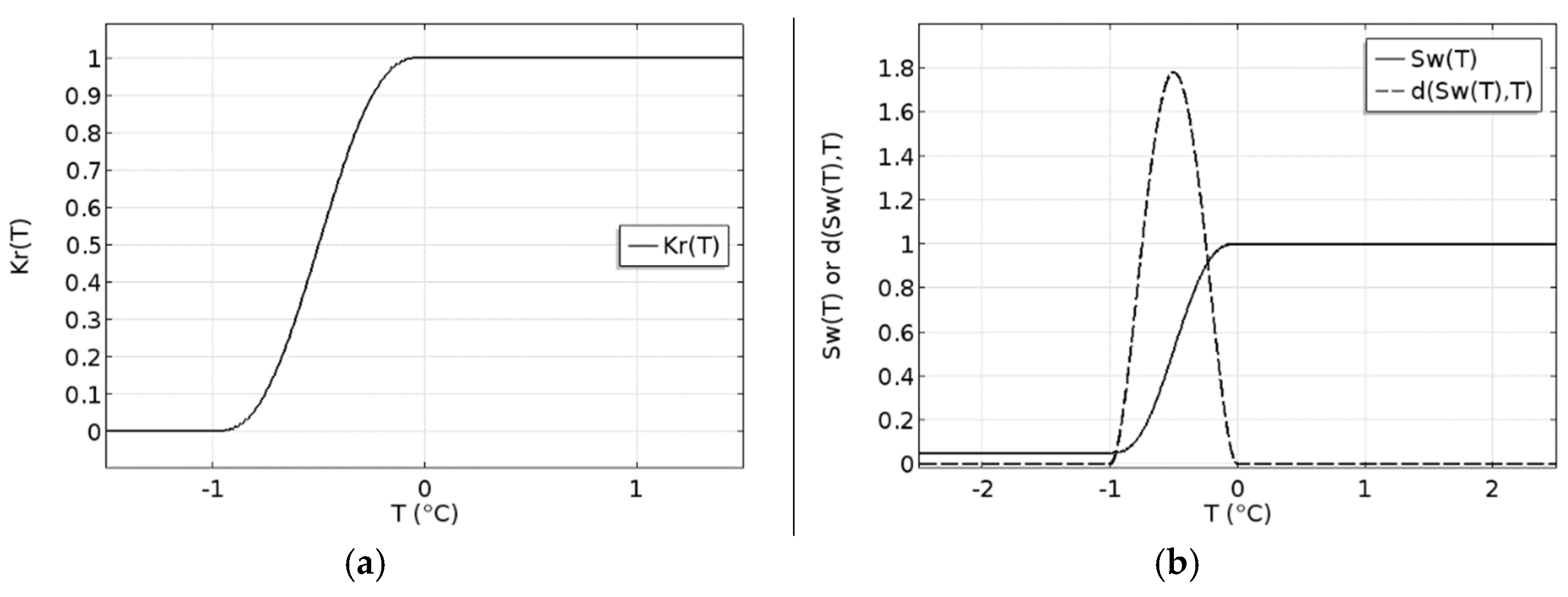
2.3. TH Coupling Parameters Description

Based on the theory of groundwater flow and heat transfer in porous media, the key coupling factors of TH governing equations are effective hydraulic conductivity and water saturation. They will have a major impact on the distribution of temperature and groundwater flow fields

2.3.1. Effective Hydraulic Conductivity

With the decreasing of temperature, the ice that forms in the pore will block the original groundwater flow channel and it results in lower soil permeability. The effective hydraulic conductivity, defined as a function of temperature, is introduced to describe this permeability reduction. Related research shows that the hydraulic conductivity during freezing depends on temperature and soil type [41,42,43]. The experimental results from Burt and Williams (1976) [42] show that the hydraulic conductivity will drop down to 10⁻⁴ times below the original value within a narrow temperature range below freezing point. Some other scholars describe this process by introducing the parameter of relative permeability [26,44]. The common functions that describe the relationship between the physical parameters and changing temperatures with phase change are piecewise linear function [28] and exponential expression [26,29]. In addition to the well-known geotechnical software GeoStudio [45], numerical software using the smoothed step function to describe parameter changes during phase transitions is less common. Due to the release of latent heat during the ice-water phase change, the nonlinearity of the convection-diffusion equation is strengthened. In this paper, we adopt smoothed Heaviside step function to characterize the relationship between permeability and temperature. The effective hydraulic conductivity is defined as

$$k_{ef}=\left(1-k_r\right)flc2hs\left(T-T_p,\delta T\right)+k_r$$

(6)

where $k_r$ is residual hydraulic conductivity, i.e. the hydraulic conductivity in the frozen body, and it is usually set very small but cannot be equal to zero; and, flc2hs represents the smoothed Heaviside function with a continuous second derivative without overshoot, which is a built-in step-function in COMSOL. The function flc2hs(x,d) is equal to 0 for x < −d, and to 1 for x > d. In between (−d < x < d), the function goes from 0 to 1, and at x = 0, flc2hs = 0.5 (more details refer to [29]); $T_p$ is the freezing point; and, $\delta T$ is the radius of the phase transition interval.

2.3.2. The Function of Water Saturation and Freezing

The function of water saturation describes the changing water content in the pores during the phase change. Obviously, it is affected by temperature and therefore a function of temperature. The saturated soils in the unfrozen zone are filled with water in their pores. In this case, the water saturation is 1. As the soil temperature drops below the freezing point of pure water, phase change of the pore water will take place, resulting in a gradual decrease in water saturation. Due to the presence of a certain amount of dissolved salt in the groundwater, the purification effect of ice causes a gradual increase of pore water concentration in the local area. In addition, some of the water exists in the form of a thin film. Hence, when more water turns into ice, the capillary and the absorption force will be enlarged, which makes it harder for the water to freeze [46]. As a result, some super-cooled unfrozen water remains in the frozen zone ($S_{rw}$). Besides the descriptions with linear function, some scholars use exponential functions to describe the residual saturation [15,34]. In order to facilitate the numerical model, the water saturation function is described by the following Heaviside function,

$$S_w=\left(1-S_{rs}\right)flc2hs\left(T-T_p,\delta T\right)+S_{rw}$$

(7)

The freezing function is used to determine the amount of released latent heat in Equation (3) during the phase change, as $-\partial S_w/\partial T$.

2.4. Numerical Implementation

The numerical implementation of the mathematical model is performed through the finite element numerical software COMSOL Multiphysics^®. This software can provide an interface between the interconnected variables of different physical fields. In the study of Scheidegger et al. (2017) [29], the TH coupling permafrost model was also established with this software. Compared with the permafrost model in their study, our AGF model faces a more complicated TH coupling process (mainly reflected in the interactional influence of freezing front shape and seepage velocity). In order to characterize this process, the numerical calculation requires much more detailed grids, especially at the vicinity of the freezing front. In our numerical study, we therefore utilized the self-adapting gridding function to initialize the detailed finite elements in order to improve the convergence of the model. Two smoothed step functions are used to describe the change of effective thermal conductivity and unfrozen water saturation with changing temperature, respectively, with the expectation that the non-linearity at the freezing front could be decreased. The feasibility of the new functions will be verified through the subsequent analytical solution and the case study of the engineering project. Previous experience has shown the obvious advantages of this software in solving complex models of coupled multi-physics. Therefore, the numerical solution of the artificial ground freezing method combined with groundwater flow in this paper is implemented in a COMSOL model, which is based on a full coupling of temperature and flow fields by combining the physical interfaces of Darcy's Law and Heat Transfer in Porous Media. The effective hydraulic conductivity ($k_r$) and the function of water saturation ($S_w$) and its derivative with respect to T ($\partial S_w/\partial T)$ in this model are defined with the smoothed step function. The relationships between them and various temperatures are shown in Figure 2.

3. Validation and Simulation Studies

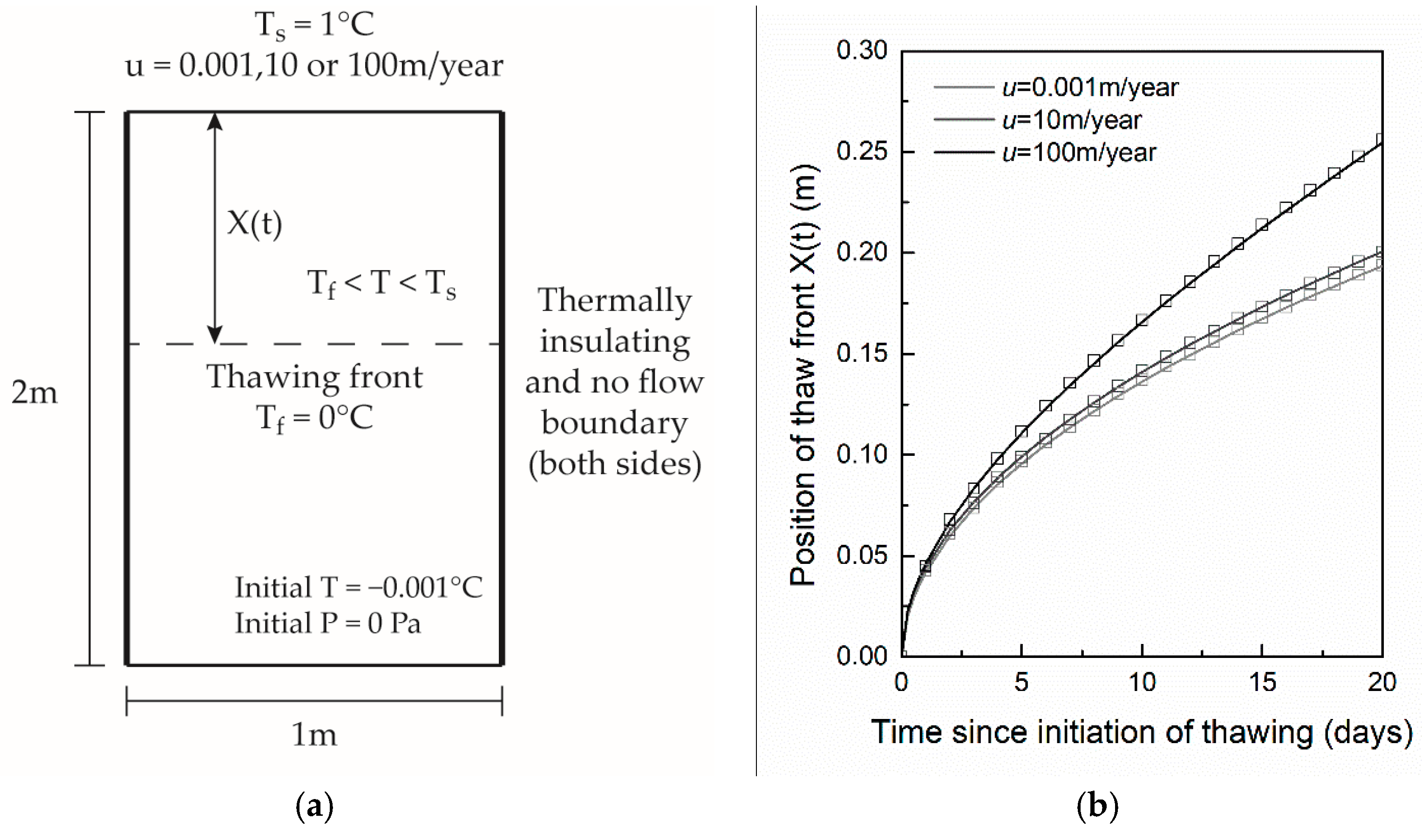
3.1. Comparison with Analytical Solution Based Results

The established numerical model for the heat transfer with phase change is verified by comparing the numerically calculated temperature with the results that are based on the classical analytical solution of freezing temperature field proposed by Lunardini (1985) [27] (hereafter referred to as the “Lunardini solution”). The Lunardini solution is firstly developed to solve a one-dimensional, semi-infinite soil thawing problem. It accommodates heat advection via water flow. In the study of Kurylyk et al. (2014) [28], the authors compared their numerical results with this analytical solution. In this study, we also use this analytical solution to validate our numerical model. The employed geometry, initial conditions, and boundary conditions in this study are shown in Figure 3. The detailed physical parameters of materials are given by Kurylyk et al. (2014) [28].

To verify the performance of this model at different groundwater flow velocities, we specified three different boundary conditions at the top: 0.001 m/year, 10 m/year, 100 m/year. The comparison of the results of analytical and numerical solutions shows a good consistency in Figure 3, which indicates that this numerical model is reliable for solving the heat transfer problem with phase change and existing groundwater flow. Beyond this, this model will be further verified by the in-situ case study in Section 4.

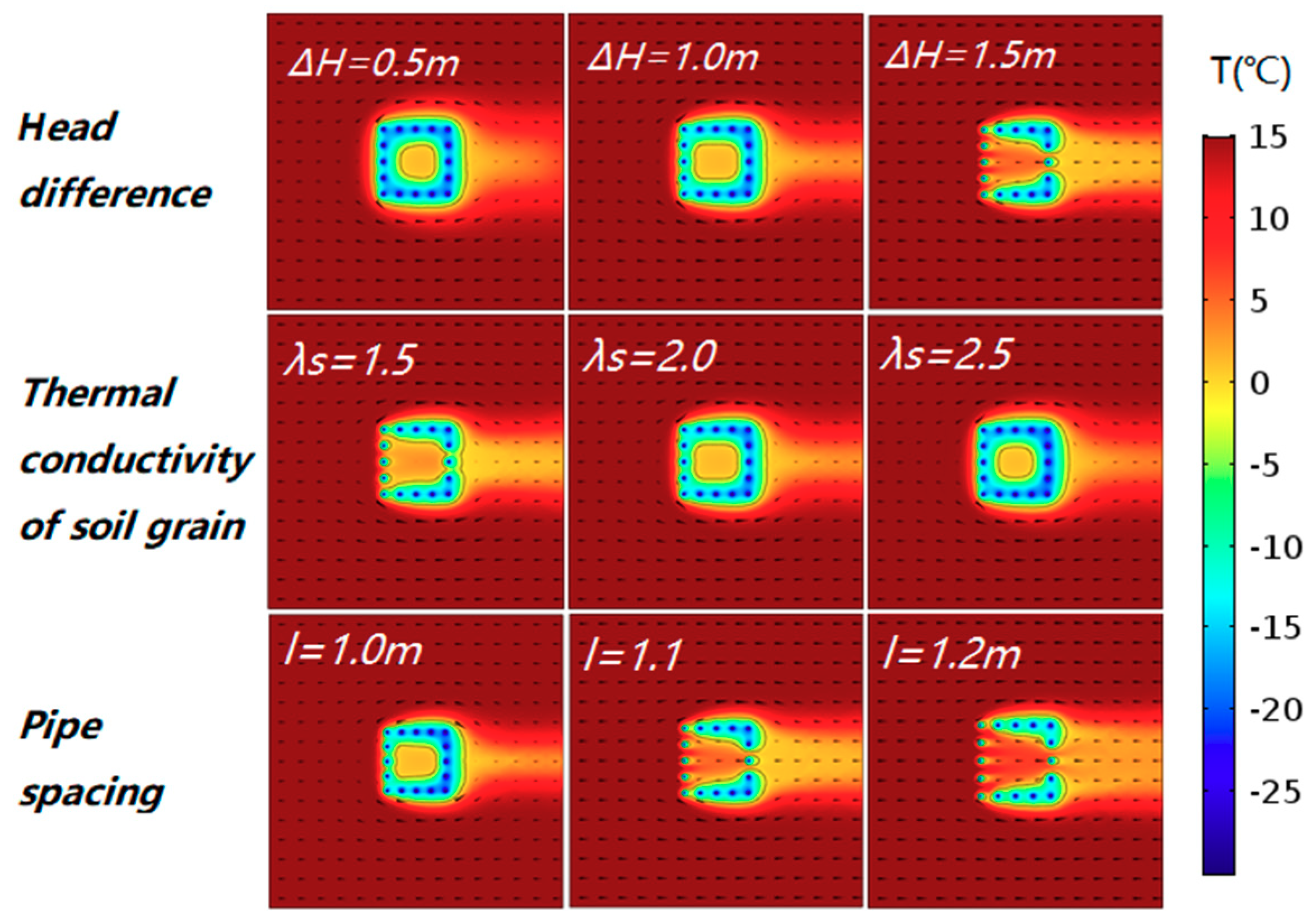
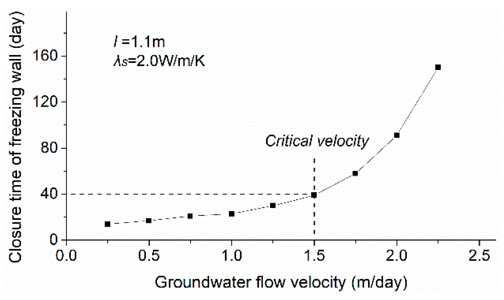
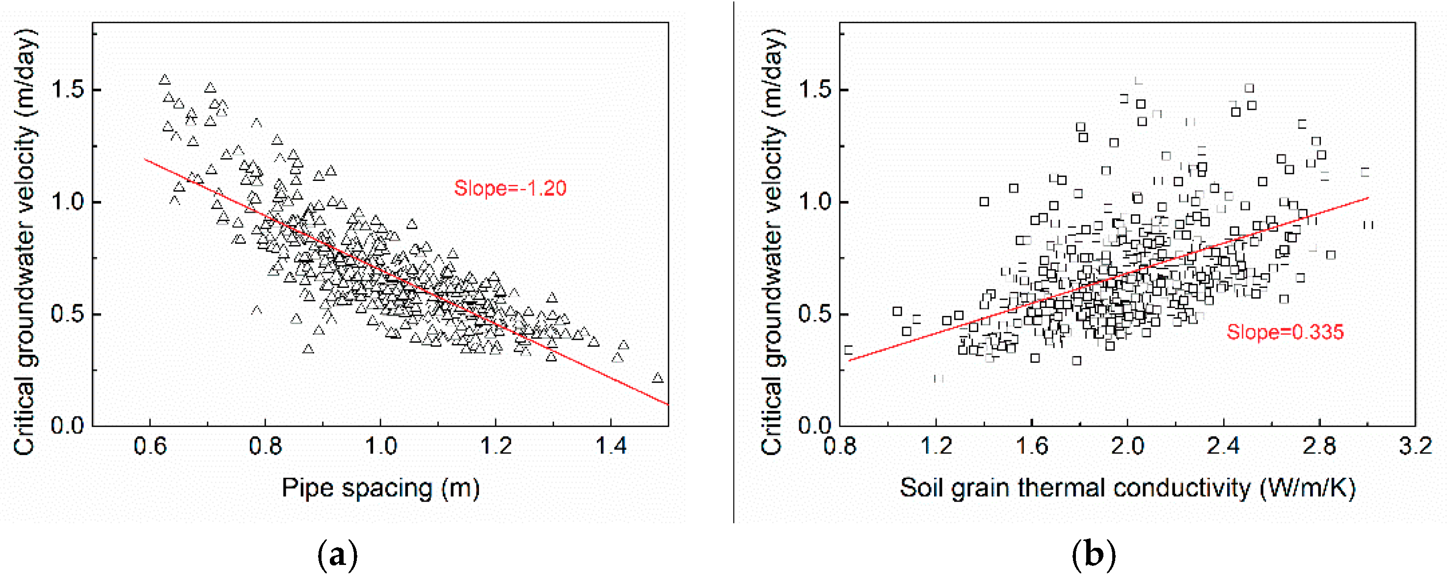
3.2. Simulation Studies

Groundwater flow will affect the soil temperature distribution in the freezing process. During this process, the groundwater flow rate is one of the key factors. A large amount of research work has been done on the influence of the groundwater flow rate on the closure time of the freezing wall [27,37,47,48,49]. However, apart from the groundwater flow rate, other parameters, such as pipe spacing, thermodynamic parameters, and so on are also important factors that affect the freezing temperature field [50]. In our study through a series of numerical experiments, we simulate and analyze the effects of pipe spacing, thermal conductivity of soil particles, and groundwater flow velocity on the temperature distribution and the closure time of the freezing wall. The geometric model used in the numerical experiment is shown in Figure 4. The 16 freezing pipes are arranged in a square with the same pipe radius of r₀ = 0.054 m. The ambient temperature $(T_0)$ is 15 °C and the initial hydraulic head has a difference of =0.8 m ($\Delta H)$ between left and right boundary. The temperature of the freezing pipes ($T_p$) is −30 °C. For detailed parameter setup, please refer to

Table 1. Parameters used in numerical experiments.

Parameters	Value
Density of Soil ${\rho }_s$(kg/m3)	2600
Density of Water ${\rho }_w$ (kg/m3)	1000
Density of Ice ${\rho }_i$ (kg/m3)	920
Pipe Spacing $l$ (m)	1.0, 1.1, 1.2 1
Head Difference $\Delta H$ (m)	0.5, 1.0, 1.5 1
Thermal Conductivity of Soil Grain ${\lambda }_s$ (W/(m·K))	1.5, 2.0, 2.5 1
Thermal Conductivity of Water ${\lambda }_w$ (W/(m·K))	0.6
Thermal Conductivity of Ice ${\lambda }_i$ (W/(m·K))	2.14
Heat Capacity of Soil $c_s$ (J/(kg·K))	840
Heat Capacity of Water $c_w$ (J/(kg·K))	4200
Heat Capacity of Ice $c_i$ (J/(kg·K))	2100
Porosity $n$	0.3
Permeability Coefficient $k$ (m/day)	20
Latent Heat of Formation $L$ (J/kg)	334,720

Note: ¹ Value for parametric sweep.

.

Based on the numerical model introduced above, three sets of parametric sweep experiments are designed for three factors, which are the head difference ($\Delta H$), thermal conductivity of soil grain (${\lambda }_s$), and pipe spacing ($l$): (1) when $l$= 1.1 and ${\lambda }_s$= 2.0, $\Delta H$ values are 0.5, 1.0, 1.5; (2) when $l$= 1.1 and $\Delta H$= 1.0, the ${\lambda }_s$ values are 1.5, 2.0, 2.5; and, (3) when $\Delta H$= 1.5 and ${\lambda }_{s }$= 2.0, the values of $l$ are 1.0, 1.1, 1.2 (for the individual unit please refer to Table 1). The experimental results of temperature distribution are shown in Figure 5. Parametric sweep results show that as the head difference and pipe spacing increase, the formation of freezing walls becomes more difficult. On the contrary, as the thermal conductivity of soil grain increases, the thickness of the frozen wall gradually increases.

Except for the shape of the frozen wall, the closure time of the frozen wall is the key factor in evaluating the ground freezing project. The case studies introduced above show that the parameters of ${\lambda }_s$, $l$, and $\Delta H$ have an important influence on the closure time, among which the roles of ${\lambda }_s$ and $l$ are explicit. The third parameter, $\Delta H$, is the controlling factor of the groundwater velocity. The influence of groundwater velocity on the ground freezing process has been discussed for years. In the ground freezing project, if the groundwater flow exceeds a certain speed, which is defined as the critical velocity, the freezing wall will not be able to close. However, this definition is difficult to quantify, as it is essentially an economic problem. As shown in Figure 6, the closure time increases exponentially with increasing groundwater flow velocity, especially after the velocity has exceeded 1.5 m/day.

In order to study further the determination and influence of critical velocity, we firstly consider the fact in our case that the freezing wall is planned to be closed within 40 days and define the allowed maximum groundwater flow velocity as the critical velocity. As shown in Figure 6, when $l$= 1.1 and ${\lambda }_{s }$= 2.0, the critical velocity is 1.5 m/day. Subsequently, we set these two parameters within certain ranges ($l\in \left[0.5,1.5\right],{\lambda }_s\in \left[1.0,3.0\right]$) and randomly sample 500 pairs of data to calculate numerically the corresponding critical velocity values. With respect to this critical value, linear regression analyses of pipe spacing and thermal conductivity are performed, and the results are shown in Figure 7. The slope of the regression line indicates that the pipe spacing is negatively correlated to the critical velocity and has more influence on the critical velocity than the thermal conductivity. As shown in Figure 7a, the degree of dispersion with a lower pipe spacing value (smaller than 0.8 m) has an increasing trend, which indicates that the pipe spacing value is no more linearly correlated to the critical velocity. On the contrary, as shown in Figure 7b, the sampling points become more scattered with increasing thermal conductivity. This indicates that, when the thermal conductivity value becomes larger, the critical velocity becomes less sensitive to it. Based on both figures, the critical velocity can be mainly found within the range of 0.25 m/day~1 m/day. If the groundwater velocity does not exceed 1 m/day, in most (about 90.6%) cases the freezing wall should be able to close within 40 days. Once exceeded, extra measures (e.g., lowering the freezing temperature, decreasing the pipe spacing, etc.) should be taken to ensure the closure of the freezing wall.

4. Engineering Application

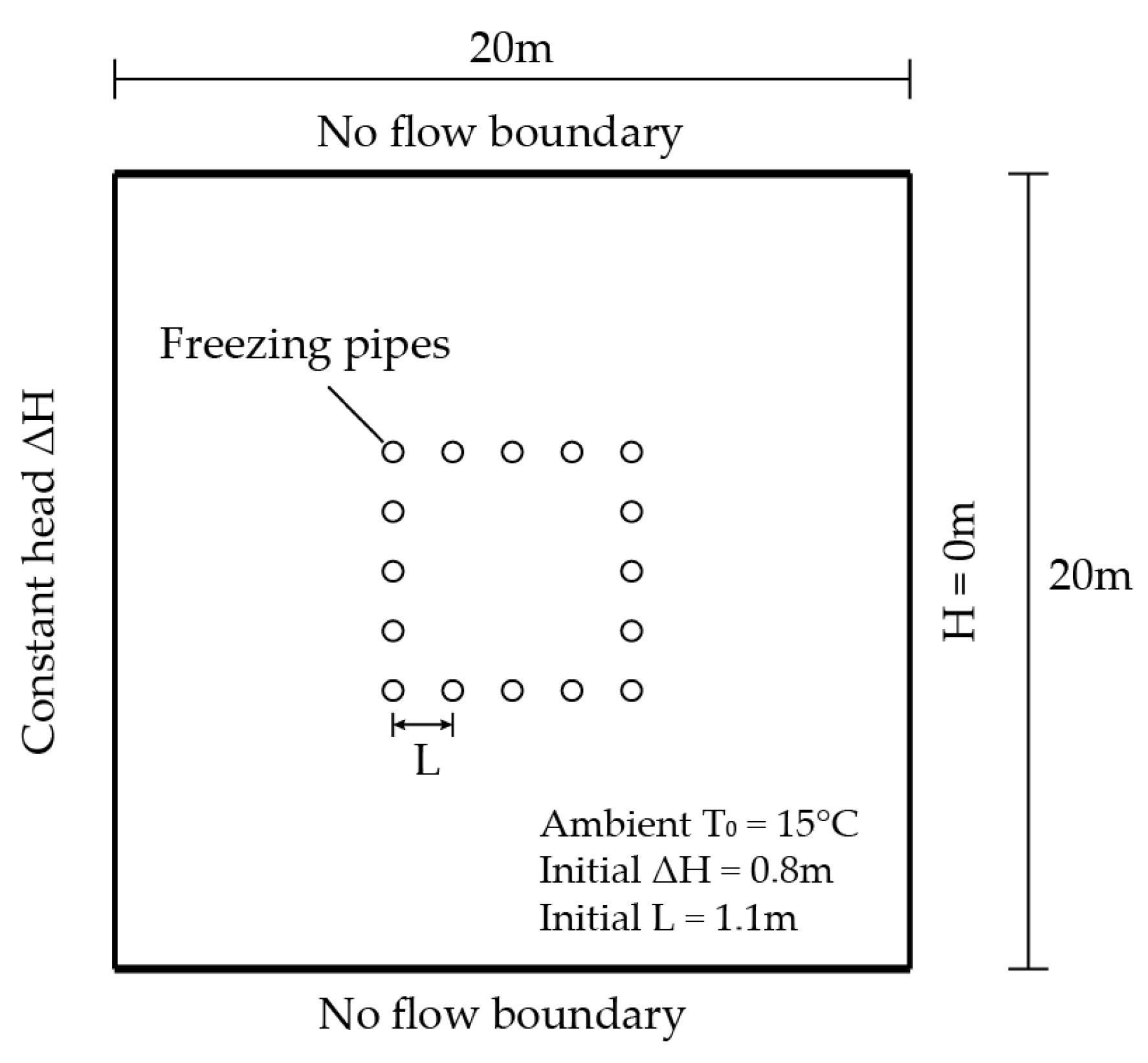
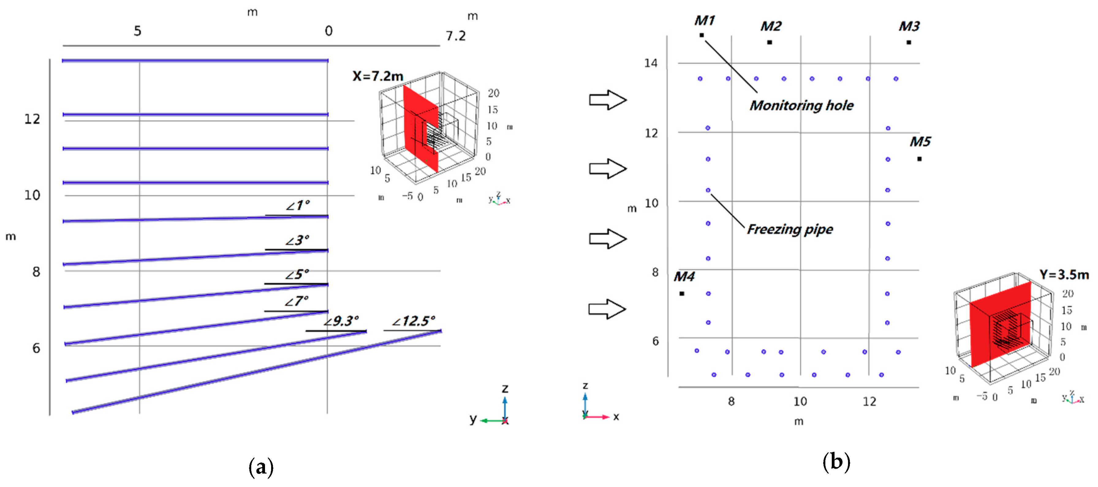
4.1. Engineering Background and the 3D Model

The application case of this study is an AGF strengthening project for the jointing section of a tunnel and a subway station located in Southern China. According to the geological survey, a saturated aquifer is at the depth of the frozen zone with silty fine sand. According to the in-situ groundwater flow test, the horizontal groundwater flow (the arrows shown in the Figure 8b) is from the left to the right side almost perpendicular to the crosscut of the tunnel. In this AGF project, 35 frozen pipes are arranged with the diameter of 108 mm each, the designed pipe spacing 1.1 m, and the length of ca. 7 m each. According to the in-situ measurements, the arrangement of freezing pipes and monitoring the hole is shown in Figure 8. The 3D model has a geometry of 20 m × 20 m × 15 m, in which the excavated tunnel is 8 m × 7.5 m × 5 m.

4.2. Boundary and Intial Conditions

According to the prior in-situ temperature monitoring data at the desired freezing depth, the initial ground temperature is about 15 °C. The box chart of initial temperatures in different thermo-observation holes is shown in Figure 9.

The lateral wall of the freezing pipe is the cooling source of the freezing system. The change in lateral wall temperature has a great effect on the temperature distribution in the whole system. The temperature monitoring values of the main-pipe, through which the refrigerant can flow to the freezing wall, can be used to represent the lateral wall temperature. According to the measured temperature of the loop main-pipe ($T_{out}$) during the freezing period (50 days), the lateral wall temperature change curve is shown in Figure 10.

The groundwater velocity obtained through the in-situ field test is 0.5 m/day. Based on Darcy’s law, the head difference between up and downstream boundary is calculated as 0.8 m.

The parameters used for the engineering example in this model is shown in

Table 2. Parameters used for engineering example.

Parameters	Value
Density of Soil ${\rho }_s$(kg/m3)	1800
Density of Water ${\rho }_w$ (kg/m3)	1000
Density of Ice ${\rho }_i$ (kg/m3)	920
Head Difference $\Delta H$ (m)	0.8
Thermal Conductivity of Soil Grain ${\lambda }_s$ (W/(m·K))	0.73
Thermal Conductivity of Water ${\lambda }_w$ (W/(m·K))	0.6
Thermal Conductivity of Ice ${\lambda }_i$ (W/(m·K))	2.14
Heat Capacity of Soil $c_s$ (J/(kg·K))	1020
Heat Capacity of Water $c_w$ (J/(kg·K))	4200
Heat Capacity of Ice $c_i$ (J/(kg·K))	2100
Porosity $n$	0.4
Permeability Coefficient $k$ (m/day)	5
Latent Heat of Formation $L$ (J/kg)	334,720

.

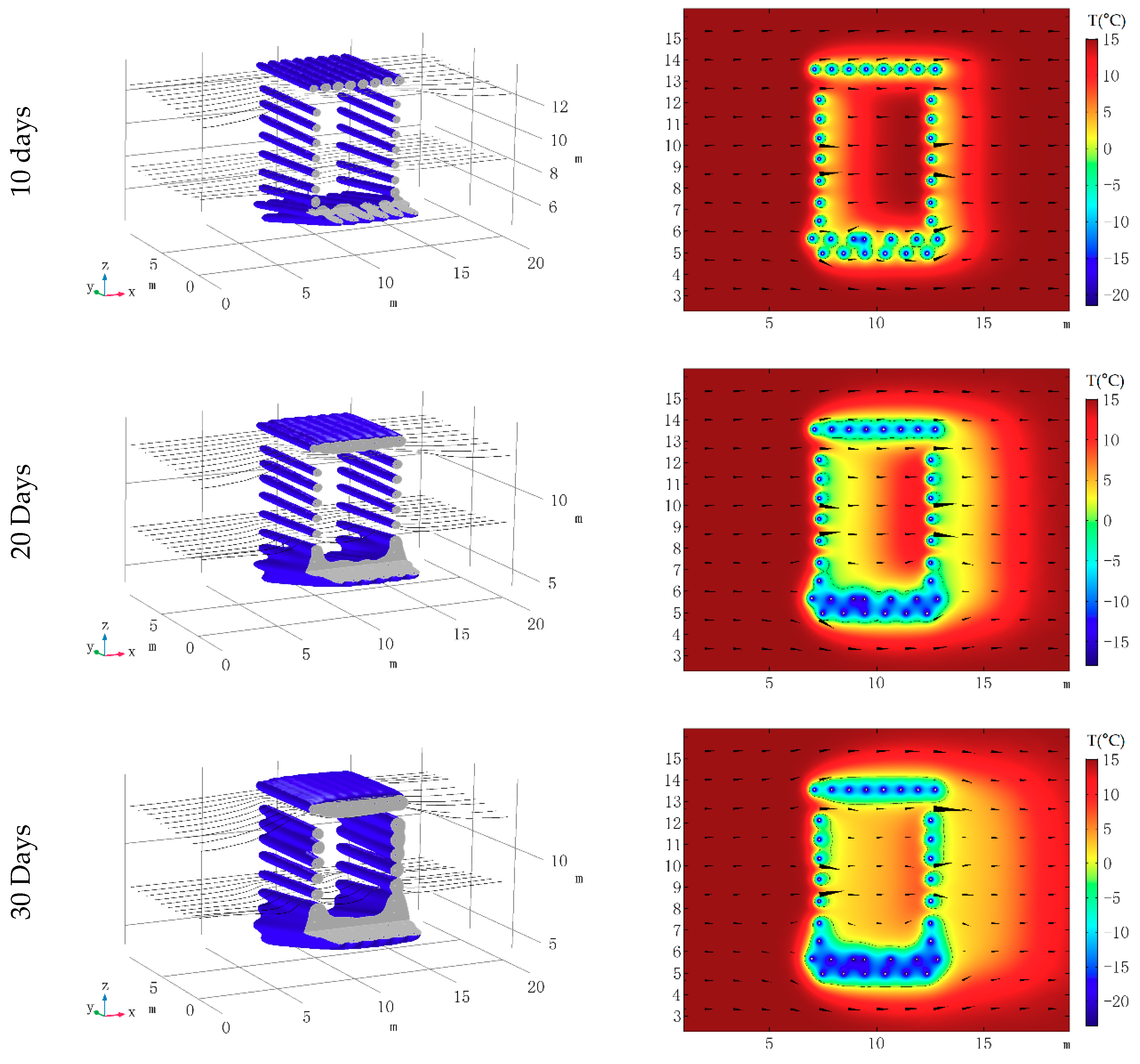
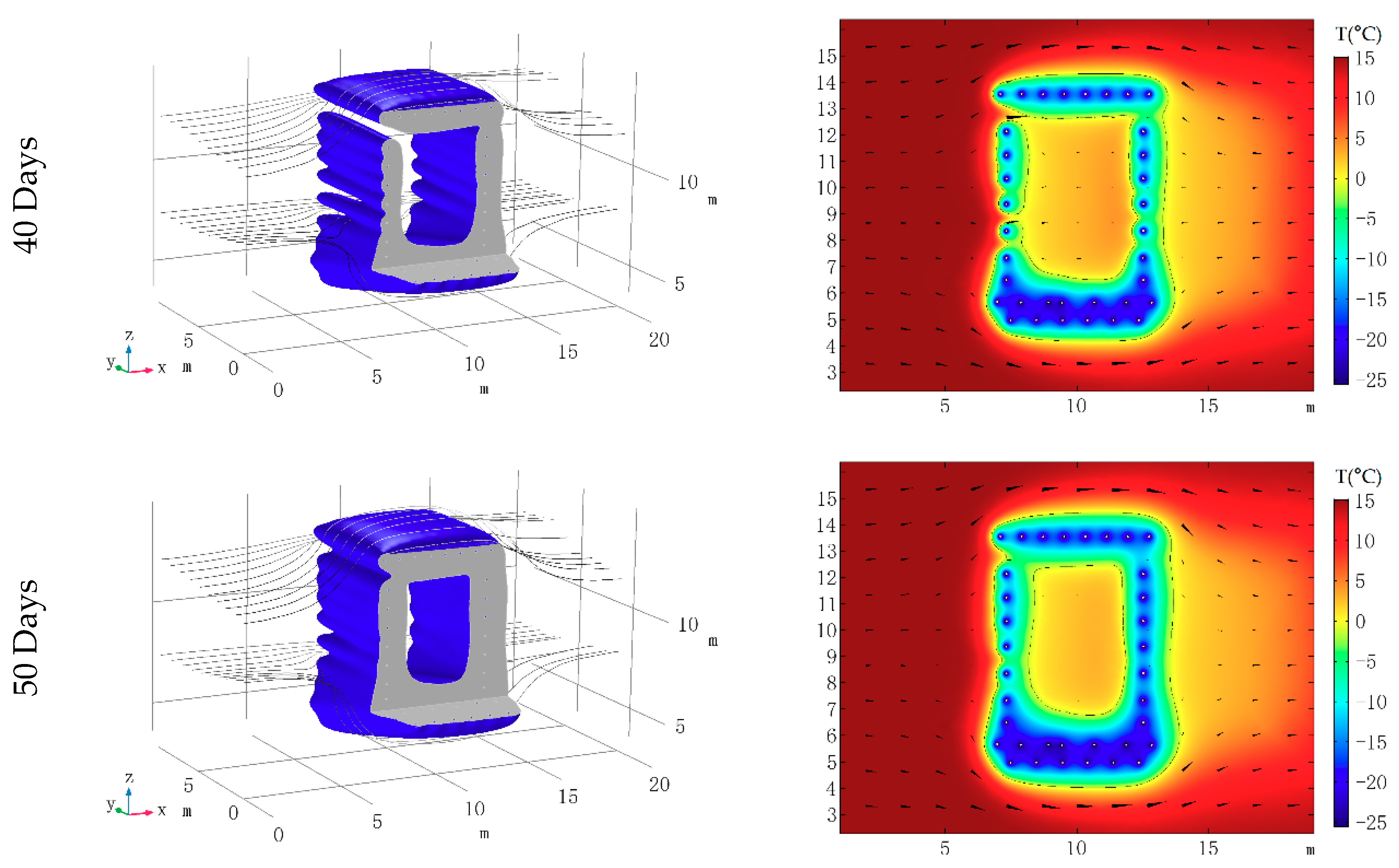
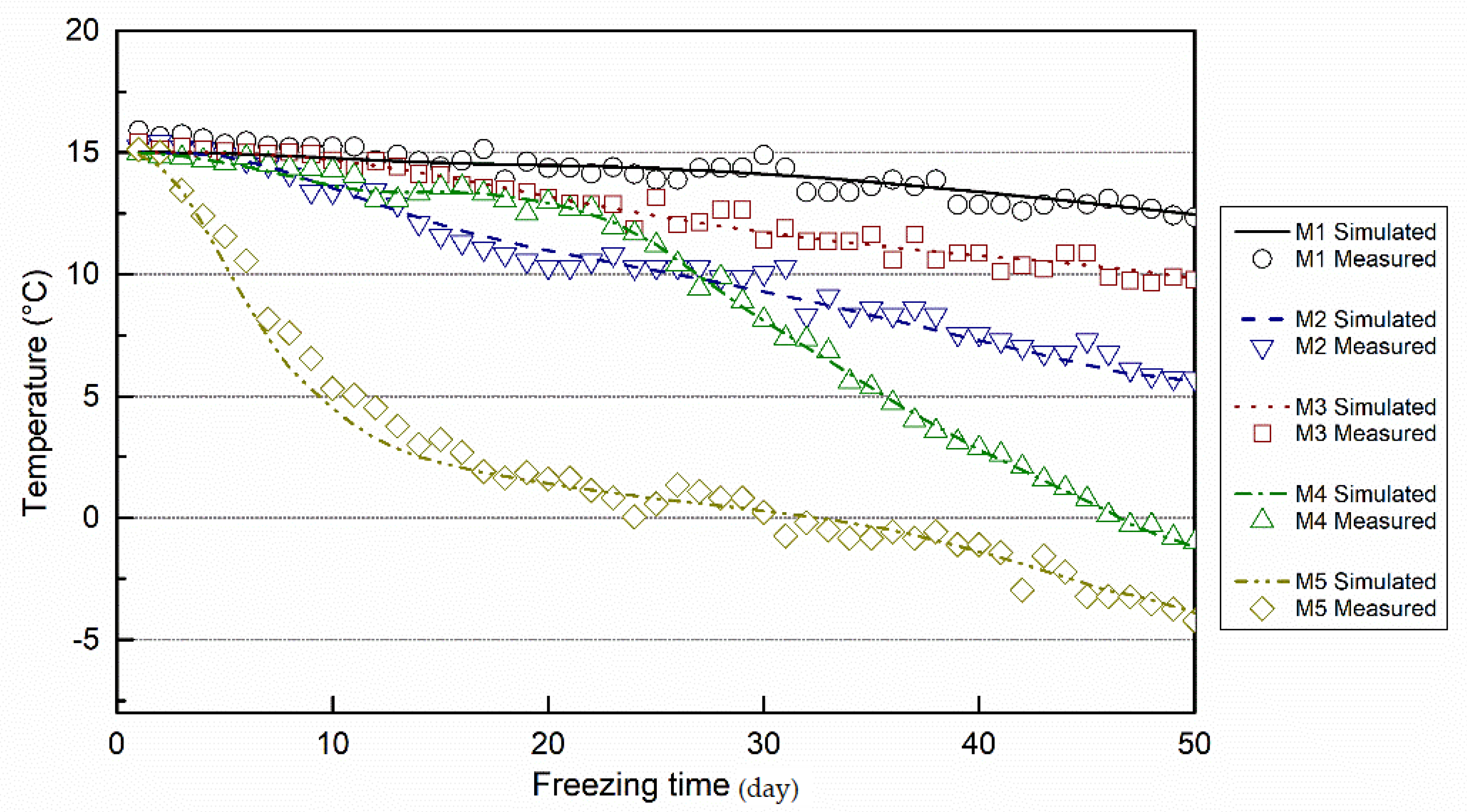
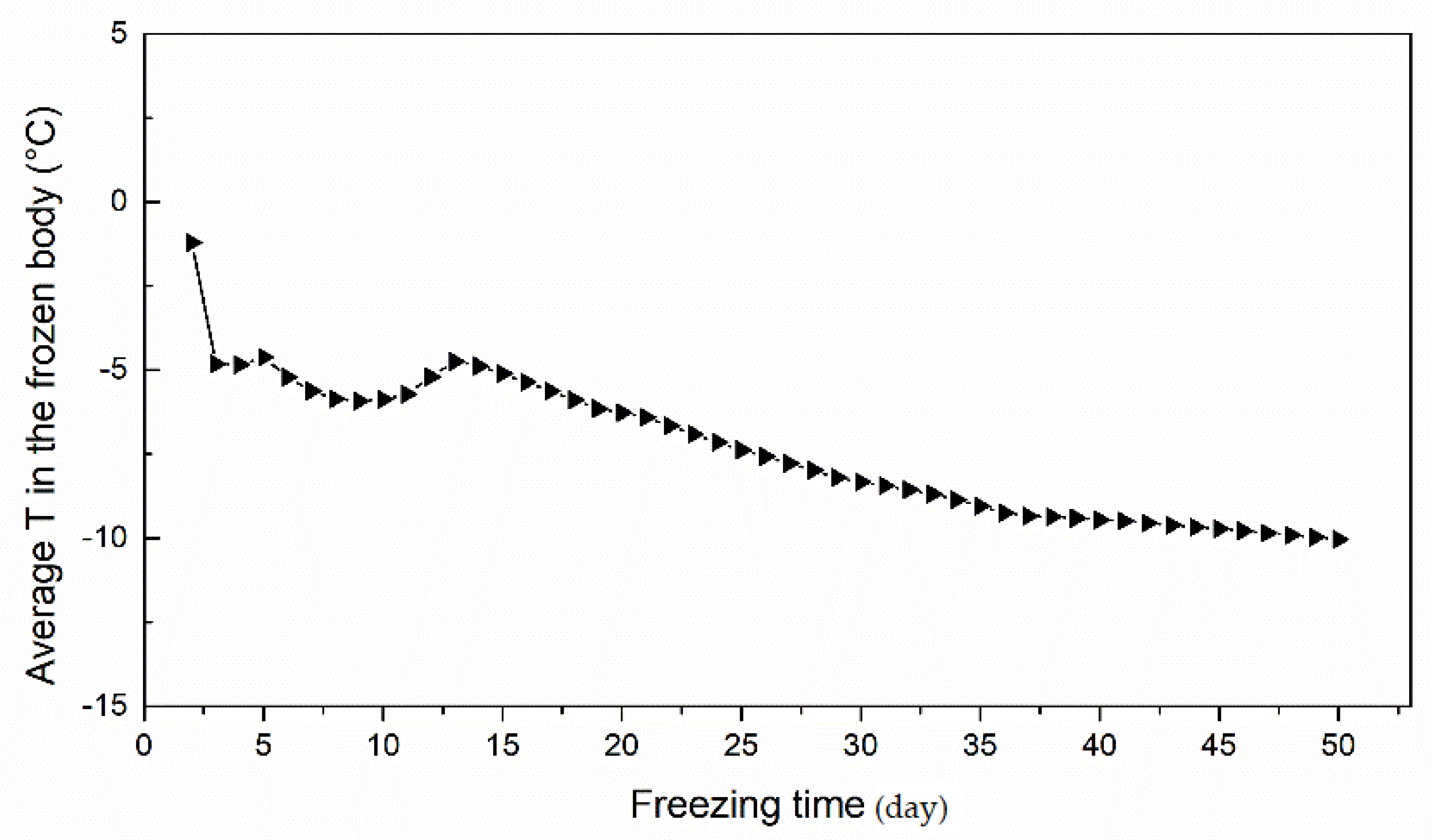
4.3. Simulation Results, Verification and Discussion

The simulation results of the temperature distribution and freezing body development at various times (10 days, 20 days, 30 days, 40 days, and 50 days) are shown in Figure 11. The freezing body and streamlines development show a clear coupling effect of groundwater flow field and the freezing temperature field. After 50 days, the freezing wall has been completely closed. But, the thickness of the frozen wall at the upstream side (left side) is relatively thin, especially at the junction of this side to the top of the frozen wall (top left corner). The simulated temperature of the freezing wall at the section of Y = 3.5 m shows obvious non-uniform distribution. Due to the arrangement of freezing pipes and the groundwater flow, the temperatures at the top and bottom of the frozen wall are lower than those at both sides of the up- and downstream. The actual pipe spacing has an important influence on the temperature field and the closure time of the freezing wall. For example, at the upper left corner of the freezing circle, the decrease of temperature is slower, resulting in a slower closing process.

According to the study in Section 3.2, the freezing wall should be able to close within 40 days if the groundwater velocity is 0.5 m/day, the soil thermal conductivity is 2.14 W/(m·K), and the pipe spacing is around 1 m. However, Figure 11 shows a closure time of 50 days. On the 40th day the freezing wall was not yet completely closed. This is due to the fact that the freezing pipes are not uniformly distributed and the pipe spacing values vary. For example, at the upper left corner the pipe spacing is 1.5 m, while at the bottom, the smallest distance between the pipes is only 0.5 m. As the frozen wall was built on the other side, and therefore the groundwater flow was limited for the left side, the unfrozen area went frozen in the next 10 days after the 40th day.

The comparison between the in-situ measured and the numerically calculated temperatures at the five monitoring points (positions shown in Figure 8) is shown in Figure 12. After the 50-day freezing period, the temperature changes of the top three monitoring points (M1, M2, M3) are relatively gentle and among which the middle measuring point M2 has a lower temperature than M1 and M3. Both monitoring points at the upstream side (M4) and the downstream side (M5) have reached below 0 °C after 50 days of freezing. The temperature of the downstream monitoring point decreased more rapidly and reached 0 °C earlier than the upstream monitoring point. Overall, the calculated curves of the temperatures at the monitored points coincide with the ones that are measured in-situ.

The average temperature of the frozen body is one of the most important indices to evaluate the strength of the frozen wall. According to the calculated results, the curve of the average temperature of the frozen wall is plotted against time in Figure 13. The results show that the average temperature change of the frozen wall coincides with that of the main frozen pipes (Figure 10) with the same trend. After a 50-day freezing period, the average temperature of the frozen body reached below −10 °C.

5. Conclusions

In this study, based on the theories of heat transport and groundwater flow in a porous medium, we set up a fully coupled numerical model with finite element software COMSOL Multiphysics^®. The coupled process of heat transport and groundwater flow with phase change was simulated. Through the model validation with an analytical solution, the sensitivity analysis, as well as the simulation of a field example with in-situ measurement data, we have drawn the following conclusions.

During the phase change, the effective hydraulic conductivity and the saturation of unfrozen water are functions of the temperature that controls the heat transport process. This function is generally described with a piecewise linear function. In this paper, we decided to use the smoothed step function. The comparison of numerically calculated and analytically solved results, as well as the validation of the field model have shown that it is feasible to use the smoothed step function to describe the change of effective hydraulic conductivity $k_r$ and the saturation of unfrozen water $S_w$ during the phase change.

With numerical case studies, sensitivity analysis was performed for three parameters: head difference ($·H$), thermal conductivity of soil grain (${\lambda }_s$), and pipe spacing ($l$). The corresponding influence of these parameters on the critical groundwater flow velocity was analyzed. The results show that when the groundwater flow velocity is within a range of 0.25 m/day~1.0 m/day, in about 90% of cases the freezing wall can be closed within 40 days. Extra measures are recommended to ensure the closure of the freezing wall, if the groundwater flow velocity exceeds this range.

The 3D model for the field example with further validation has shown that, along the groundwater flow direction, the freezing wall forms slowly and on the upstream side the thickness of the freezing wall is thinner than on the downstream side. The actual pipe spacing has an important influence on the temperature field and closure time of the freezing wall. The larger the actual pipe spacing is, the slower the closing process will be. Besides this, the average temperature change of the freezing body coincides with that of the main frozen pipes with the same trend.

References

1. Gallardo, A.H.; Marui, A. The aftermath of the Fukushima nuclear accident: Measures to contain groundwater contamination. Sci. Total Environ. 2016, 547, 261–268. [Google Scholar] [CrossRef] [PubMed]
2. Dash, J. Ground freezing technology for environmental. Ice Phys. Nat. Environ. 2013, 56, 241. [Google Scholar]
3. Wallis, S. Freezing under the sea rescues oslofjord highway tunnel. Tunnel 1999, 8, 19–26. [Google Scholar]
4. Hu, X.D.; Zhang, L.Y. Artificial Ground Freezing for Rehabilitation of Tunneling Shield in Subsea Environment; Advanced Materials Research; Trans Tech Publications: Zurich, Switzerland, 2013; pp. 517–521. [Google Scholar]
5. Papakonstantinou, S.; Anagnostou, G.; Pimentel, E. Evaluation of ground freezing data from the Naples subway. Proc. Inst. Civ. Eng. Geotech. Eng. 2013, 166, 280–298. [Google Scholar] [CrossRef]
6. Marwan, A.; Zhou, M.-M.; Abdelrehim, M.Z.; Meschke, G. Optimization of artificial ground freezing in tunneling in the presence of seepage flow. Comput. Geotech. 2016, 75, 112–125. [Google Scholar] [CrossRef]
7. Russo, G.; Corbo, A.; Cavuoto, F.; Autuori, S. Artificial ground freezing to excavate a tunnel in sandy soil. Measurements and back analysis. Tunnelling Underground Space Technol. 2015, 50, 226–238. [Google Scholar] [CrossRef]
8. Haß, H.; Schäfers, P. International Symposium on Geotechnical Aspects of Underground Construction in Soft Ground. In Application of Ground Freezing for Underground Construction in Soft Ground; Taylor & Francis London: Oxfordshire, UK, 2005; pp. 405–412. [Google Scholar]
9. Colombo, G.; Lunardi, P.; Cavagna, B.; Cassani, G.; Manassero, V. The artificial Ground Freezing Technique Application for the Naples Underground. In Proceedings of the Word Tunnel Congress, Agra, India, 22–24 September 2008. [Google Scholar]
10. Vitel, M.; Rouabhi, A.; Tijani, M.; Guérin, F. Thermo-hydraulic modeling of artificial ground freezing: Application to an underground mine in fractured sandstone. Comput. Geotech. 2016, 75, 80–92. [Google Scholar] [CrossRef]
11. Pimentel, E.; Sres, A.; Anagnostou, G. Large-scale laboratory tests on artificial ground freezing under seepage-flow conditions. Géotechnique 2012, 62, 227. [Google Scholar] [CrossRef]
12. Arenson, L.U.; Sego, D.C. Freezing Processes for a Coarse sand with Varying Salinities. In Proceedings of the Cold Regions Engineering & Construction Conference, Edmonton, Alta, 16–19 May 2004. [Google Scholar]
13. Bing, H.; Ma, W. Laboratory investigation of the freezing point of saline soil. Cold Reg. Sci. Technol. 2011, 67, 79–88. [Google Scholar] [CrossRef]
14. Frivik, P.; Comini, G. Seepage and heat flow in soil freezing. J. Heat Transf. 1982, 104, 323–328. [Google Scholar] [CrossRef]
15. Nishimura, S.; Gens, A.; Olivella, S.; Jardine, R. THM-coupled finite element analysis of frozen soil: Formulation and application. Géotechnique 2006. [Google Scholar] [CrossRef]
16. Lai, Y.; Pei, W.; Zhang, M.; Zhou, J. Study on theory model of hydro-thermal–mechanical interaction process in saturated freezing silty soil. Int. J. Heat Mass Transf. 2014, 78, 805–819. [Google Scholar] [CrossRef]
17. Yang, P.; Ke, J.-M.; Wang, J.; Chow, Y.; Zhu, F.-B. Numerical simulation of frost heave with coupled water freezing, temperature and stress fields in tunnel excavation. Comput. Geotech. 2006, 33, 330–340. [Google Scholar] [CrossRef]
18. Wu, D.; Lai, Y.; Zhang, M. Heat and mass transfer effects of ice growth mechanisms in a fully saturated soil. Int. J. Heat Mass Transf. 2015, 86, 699–709. [Google Scholar] [CrossRef]
19. Gao, J.; Feng, M.; Yang, W.-H. Research on distribution law of frozen temperature field of fractured rock mass with groundwater seepage. J. Min. Saf. Eng. 2013, 1, 013. [Google Scholar]
20. Vitel, M.; Rouabhi, A.; Tijani, M.; Guérin, F. Modeling heat transfer between a freeze pipe and the surrounding ground during artificial ground freezing activities. Comput. Geotech. 2015, 63, 99–111. [Google Scholar] [CrossRef]
21. Vitel, M.; Rouabhi, A.; Tijani, M.; Guérin, F. Modeling heat and mass transfer during ground freezing subjected to high seepage velocities. Comput. Geotech. 2016, 73, 1–15. [Google Scholar] [CrossRef]
22. Grenier, C.; Anbergen, H.; Bense, V.; Chanzy, Q.; Coon, E.; Collier, N.; Costard, F.; Ferry, M.; Frampton, A.; Frederick, J.; et al. Groundwater flow and heat transport for systems undergoing freeze-thaw: Intercomparison of numerical simulators for 2d test cases. Adv. Water Resour. 2018, 114, 196–218. [Google Scholar] [CrossRef]
23. Harlan, R. Analysis of coupled heat-fluid transport in partially frozen soil. Adv. Water Resour. 1973, 9, 1314–1323. [Google Scholar] [CrossRef]
24. Guymon, G.L.; Luthin, J.N. A coupled heat and moisture transport model for arctic soils. Water Resour. Res. 1974, 10, 995–1001. [Google Scholar] [CrossRef]
25. Hansson, K.; Šimůnek, J.; Mizoguchi, M.; Lundin, L.-C.; Van Genuchten, M.T. Water flow and heat transport in frozen soil. Vadose Zone J. 2004, 3, 693–704. [Google Scholar] [CrossRef]
26. McKenzie, J.M.; Voss, C.I.; Siegel, D.I. Groundwater flow with energy transport and water–ice phase change: Numerical simulations, benchmarks, and application to freezing in peat bogs. Adv. Water Resour. 2007, 30, 966–983. [Google Scholar] [CrossRef]
27. Lunardini, V. Freezing of soil with phase change occurring over a finite temperature difference. In Proceedings of the 4th International Offshore Mechanics and Arctic Engineering Symposium, Dallas, TX, USA, 17–21 February 1985. [Google Scholar]
28. Kurylyk, B.L.; McKenzie, J.M.; MacQuarrie, K.T.; Voss, C.I. Analytical solutions for benchmarking cold regions subsurface water flow and energy transport models: One-dimensional soil thaw with conduction and advection. Adv. Water Resour. 2014, 70, 172–184. [Google Scholar] [CrossRef]
29. British Geological Survey Commissioned Report: 2017: Coupled Modelling of Permafrost and Groundwater. A Case Study Approach; British Geological Survey: Keyworth, Nottingham, UK, 2017; p. 157.
30. Tan, X.; Chen, W.; Tian, H.; Cao, J. Water flow and heat transport including ice/water phase change in porous media: Numerical simulation and application. Cold Reg. Sci. Technol. 2011, 68, 74–84. [Google Scholar] [CrossRef]
31. Mizoguchi, M. Water, Heat and Salt Transport in Freezing Soil. Ph.D. Thesis, University of Tokyo, Tokyo, Japan, 1990. [Google Scholar]
32. Sres, A. Theoretische und Experimentelle Untersuchungen zur Künstlichen Bodenvereisung im Strömenden Grundwasser; vdf Hochschulverlag AG: Zurich, Switzerland, 2010; p. 18378. [Google Scholar]
33. Ständer, W. Mathematische Ansätze zur Berechnung der Frostausbreitung in Ruhendem Grundwasser im Vergleich zu Modelluntersuchungen für Verschiedene Gefrierrohranordnungen im Schactund Grundbau; Technische Hochschule Fridericiana, Institut für Bodenmechanik und Felsmechanik: Karlsruhe, Germany, 1967. [Google Scholar]
34. Victor, H. Die Frostausbreitung beim Künstlichen Gefrieren von Böden unter dem Einfluss Strömenden Grundwassers; Univ. Inst. f. Bodenmechanik u. Felsmechanik: Karlsruhe, Germany, 1969; p. 42. [Google Scholar]
35. Sanger, F.; Sayles, F. Thermal and rheological computations for artificially frozen ground construction. Eng. Geol. 1979, 13, 311–337. [Google Scholar] [CrossRef]
36. Huang, R.; Chang, M.; Tsai, Y.; Lu, S.; Wu, P. Influence of seepage flow on temperature field around an artificial frozen soil through model testing and numerical simulations. In Proceedings of the 18th Southeast Asian Geotechnical Conference, Singapore, 29–31 May 2013; Leung; Leung, C.F., Goh, S.H., Shen, R.F., Eds.; Geotechnical Society of Singapore, Research Publishing Services: Singapore, 2013. [Google Scholar]
37. Jessberger, H.; Jagow-Klaff, R. Bodenvereisung. Grundbau-Taschenbuch, Teil 2: Geotechnische Verfahren; Country Ernst & Sohn: Berlin, Germany, 2001; pp. 121–166. [Google Scholar]
38. Andersland, O.B.; Ladanyi, B. Frozen Ground Engineering; John Wiley & Sons: Hoboken, NJ, USA, 2004. [Google Scholar]
39. Endo, K. Artificial Soil Freezing Method for Subway Construction; Japan Society of Civil Engineers: Tokyo, Japan, 1969. [Google Scholar]
40. Zhou, X.; Wang, M.; Zhang, X. Model test research on the formation of freezing wall in seepage ground. J. Chin. Coal Soc. 2005, 30, 196–201. [Google Scholar]
41. Williams, P.; Burt, T. Measurement of hydraulic conductivity of frozen soils. Can. Geotech. J. 1974, 11, 647–650. [Google Scholar] [CrossRef]
42. Burt, T.; Williams, P.J. Hydraulic conductivity in frozen soils. Earth Surf. Process. Landf. 1976, 1, 349–360. [Google Scholar] [CrossRef]
43. Horiguchi, K.; Miller, R. Experimental studies with frozen soil in an “ice sandwich” permeameter. Cold Reg. Sci. Technol. 1980, 3, 177–183. [Google Scholar] [CrossRef]
44. Jame, Y.W.; Norum, D.I. Heat and mass transfer in a freezing unsaturated porous medium. Water Resour. Res. 1980, 16, 811–819. [Google Scholar] [CrossRef]
45. Heat and Mass Transfer Modeling with GeoStudio 2018, 2nd ed.; GEOSLOPE International Ltd.: Calgary, AB, Canada, 2017.
46. Embleton, C. The Frozen Earth: Fundamentals of Geocryology; Cambridge University Press: Cambridge, UK, 1992. [Google Scholar]
47. Ziegler, M.; Baier, C.; Aulbach, B. Optimization of artificial ground freezing application of tunneling subject to water seepage. In Proceedings of the 17th Internal Conference on Soil Mechanics and Geotechnical Engineering, Alexandria, Egypt, 5–9 October 2009. [Google Scholar]
48. Zhou, M.; Meschke, G. A three-phase thermo-hydro-mechanical finite element model for freezing soils. Int. J. Numer. Anal. Methods Geomech. 2013, 37, 3173–3193. [Google Scholar] [CrossRef]
49. Shen, C.; McKinzie, B.; Arbabi, S. A reservoir simulation model for ground freezing process. In Proceedings of the SPE Annual Technical Conference and Exhibition, Florence, Italy, 19–22 September 2010. [Google Scholar]
50. Lackner, R.; Amon, A.; Lagger, H. Artificial ground freezing of fully saturated soil: Thermal problem. J. Eng. Mech. 2005, 131, 211–220. [Google Scholar] [CrossRef]
Figure 1. Schematic of a typical phase diagram for the freezing process.
Water 10 01322 g001
Figure 2. The temperature dependent parameters employed in the numerical implementation: (a) Effective hydraulic conductivity curve with various temperatures; and, (b) The function of water saturation and freezing with various temperatures.
Water 10 01322 g002
Figure 3. Comparison of the results of analytical and numerical solutions. (a) Model geometry, initial conditions and boundary conditions employed in COMSOL; and, (b) position of the thawing front versus time at three Darcy velocities: 0.001 m/year (light gray, negligible advection), 10 m/year (medium gray), and 100 m/year (black) calculated by Lunardini’s analytical solution (lines) and numerical solution (squares).
Water 10 01322 g003
Figure 4. Model geometry, initial and boundary conditions for the simulation of the artificial ground freezing (AGF) project.
Water 10 01322 g004
Figure 5. The temperature distribution results of parametric sweep experiments.
Water 10 01322 g005
Figure 6. Closure times of freezing wall with various groundwater flow velocities and definition of the critical velocity.
Water 10 01322 g006
Figure 7. Scatter plot of changes in critical groundwater flow velocity with respect to (a) Pipe spacing; and, (b) Soil grain thermal conductivity based on 500 random sampling pairs. The red line represents the linear regression analysis.
Water 10 01322 g007
Figure 8. The arrangement of freezing pipes and monitoring points in three-dimensional (3D) model. (a) Side view with blue lines representing the freezing pipes; (b) Front view (the arrows represent groundwater flow direction).
Water 10 01322 g008
Figure 9. The box chart of initial ground temperatures in different thermo-observation holes.
Water 10 01322 g009
Figure 10. The measured temperature of the loop main-pipe during freezing period.
Water 10 01322 g010
Figure 11. The development of freezing body with streamlines (black lines) (left) and temperature distribution with velocity vector (black arrows) at Y = 3.5 m (right) at various times.
Water 10 01322 g011aWater 10 01322 g011b
Figure 12. The temperature comparison curve of monitoring points between simulated and measured values.
Water 10 01322 g012
Figure 13. Average temperature curve of the frozen body versus freezing time.
Water 10 01322 g013