Impact of Uncertainty of Floodplain Digital Terrain Model on 1D Hydrodynamic Flow Calculation

Abstract

This study investigates the effect of the Digital Terrain Model (DTM) uncertainty effect on the output of a 1D flow model. The analysis is performed for the lowland river Biebrza, covered with dense wetland vegetation, with a high uncertainty of terrain elevations. The DTM uncertainty is modeled in two ways: (1) accounting for the uncertainty spatial dependency on the basis of the correlogram function and (2) neglecting the correlation of the elevation points. The model explanation of water levels improves when elevation uncertainty is being included. Without the elevation uncertainty, the model provided a good fit only for peak flows, with uncertainty also representation of lower flows is better. It was shown that the correlation of the elevation uncertainty had a noticeable effect on the modeling outcomes, especially for near bankfull flows, where for the uncorrelated case water levels were underestimated by 5 cm, comparing to the correlated case. The effect was also present for inundation extents, obtained by an interpolation of computed water levels. The correlation of the elevation uncertainty strongly affects estimates of standard deviations of computed water levels, which were almost twice smaller when correlation was neglected. In the result, only when the correlation of the elevation uncertainty was included, it was possible to obtain confidence bands that enclosed observation points.

1. Introduction

Nowadays, many issues related to restoration, flood protection, and the functioning of aquatic ecosystems in natural river valleys are solved using hydrodynamic flow models [1,2,3,4,5]. In most cases, terrain features are being represented using Digital Terrain Models (DTM), allowing a combination of different sources of spatial data. DTM can be produced using field, aerial, satellite, or all these data sets together [6]. In flood routing, DTM are usually used to characterize floodplains, which surface can be efficiently acquired using remote sensing techniques [7,8].

In any application, the DTM can be a noticeable source of an uncertainty, for example, Mirosław-Świątek et al. [9] demonstrated that the quality of the DTM not only affects the modeling accuracy, but also determines the correctness of decisions related to river valley management, based on modeling tools. The most accurate DTM can be obtained on the basis of Light Detection and Ranging (LIDAR) techniques, while large scale assessments often benefit from less accurate but globally available satellite data, like Shuttle Radar Topography Mission (SRTM) [8,10]. There is an agreement that the uncertainty of DTMs depends on the land cover and its highest values are expected for densely vegetated areas [11,12,13,14]. For example, the Root-Mean-Squared-Error (RMSE) for low grasses is about 20 cm, while for areas covered with shrubs and trees it is even above 1 m [14,15,16].

In addition to noticeable values of RMSE, the DTM uncertainty structure reveals strong spatial correlation [17,18]. It is explained that for such regions only a small portion of reflection points is recorded for a bare-earth and the void areas are fulfilled in the DTM by interpolation [19]. Because of this, DTM errors are usually correlated: an error of a point interpolated between two other points will depend on their errors, despite the fact that elevation errors of sampled points in LIDAR or satellite imagery are expected to be independent.

In river flow modeling, DTM are recognized as a significant source of an uncertainty [20,21,22,23]. However, despite the importance of the problem, still there is just a few studies on propagation of the DTM uncertainty in flood routing methods [24,25,26,27,28,29]. Yan et al. [24] showed that the accuracy of the DTM affects the estimates of the flood inundation uncertainty, described in terms of uncertain design flows and roughness parameters. Podhoranyi and Fedorcak [25] analyzed the effect of the uncertainty of the LIDAR bathymetrical measurements on flood routing. One of the earliest studies, where the DTM uncertainty was modeled along with the uncertainty of the hydrodynamic model was performed by Jung and Merwade [26]. Applying uncorrelated distortions to each cross-section point that was obtained from the DTM, in their one-dimensional model they showed that the DTM uncertainty is a key factor in flood routing, overwhelming the uncertainty accounted to roughness parameters. The spatial dependency of the DTM uncertainty was for a first time included by Tsubaki and Kawahara [27]. They performed the uncertainty analysis of the DTM on a two dimensional (2D) flow model for a hypothetical flood scenario in an urban area, stressing the significance of spatial dependency of the elevation errors. The urban area was also a case study for Abily et al. [28] who carried out a sensitivity analysis of a two dimensional flood model for parameters used in processing of LIDAR raw data sets. The effect of the spatial dependency of the elevation uncertainties on a two-dimensional model was also investigated by Knighton [29].

Still, however, the knowledge on the significance of DTM uncertainty and its spatial correlation on flood routing methods is poorly developed. It is unsure how this source of uncertainty affects the modeling outcomes. This issue can be especially important for one-dimensional models (1D), because of the simpler representation of the river geometry, than in 2D cases. In 1D approaches a channel geometry is being parametrized using cross-sections, extracted from the DTM, perpendicular to a flow. As cross section points reveal a strong spatial dependency—floodplain elevations decrease towards river banks—the question is how the DTM uncertainty should be represented in a 1D model? Is spatial dependency important for computed water levels and inundation extents, or can it be neglected?

The above problems, including correlation of DTM uncertainty, are well recognized in geostatistical and hydrological studies. Heuvelink [30] argued that although spatial correlation of DTM uncertainty affects its ‘derivatives’ like determined slopes and aspects, neglecting it can be considered as ‘the worst case scenario’. Oksanen and Sarjakoski [31] showed, however, that the spatial correlation of the DTM uncertainty might increase uncertainty of its derivatives (slopes, aspects, and also the drainage basin delineation). Wechsler [32] provided a comprehensive review of methods of the DTM uncertainty modeling, mentioning several methods for its spatial dependency. The DTM uncertainty can be assessed using the knowledge on the error structure, identified using higher quality data for ground surveys. More often, however, such data is missing and the DTM uncertainty can be represented using a known RMSE with assumed spatial correlation models [32]. The second approach can be found, in [33] the spatial dependency of DTM uncertainty was linked with a variogram. The review of other approaches can be found in [34].

The aim of the present study is to investigate the propagation of the DTM uncertainty in a 1D flow model, accounting for the effect of its correlation. The problem is addressed using as a case study a wetland river of Biebrza. For such river valleys, covered with dense vegetation, DTMs are affected by high uncertainty [9]. Its effect on computed water levels, using a one-dimensional unsteady flow model, is investigated using two models for the DTM uncertainty: including and excluding the spatial correlation of elevation errors. Transformation of the DTM uncertainty through the flow routing model is solved using Monte Carlo sampling. Available data do not allow for a direct identification of the DTM uncertainty structure. Therefore, the uncertainty is modelled on the basis of the spatial correlation of the elevation errors, estimated with a spatial correlogram [33,35]. The study focus on propagation. It should be noticed that flood routing models are affected by other sources of uncertainty, like parametrization of roughness [26,36,37,38]. In the present study the other sources are neglected in order to focus on the DTM uncertainty.

This is one of the first studies where the effect of spatial correlation of DTM uncertainties is being analyzed for a 1D model. In the following section, the study area and DTM are introduced. Further, the methodology for flow routing and DTM uncertainty is explained. The results section shows computed uncertainties of water levels and inundation extents for different DTM uncertainty models (correlated and uncorrelated). The outcomes are discussed in the Discussion section.

2. Materials and Methods

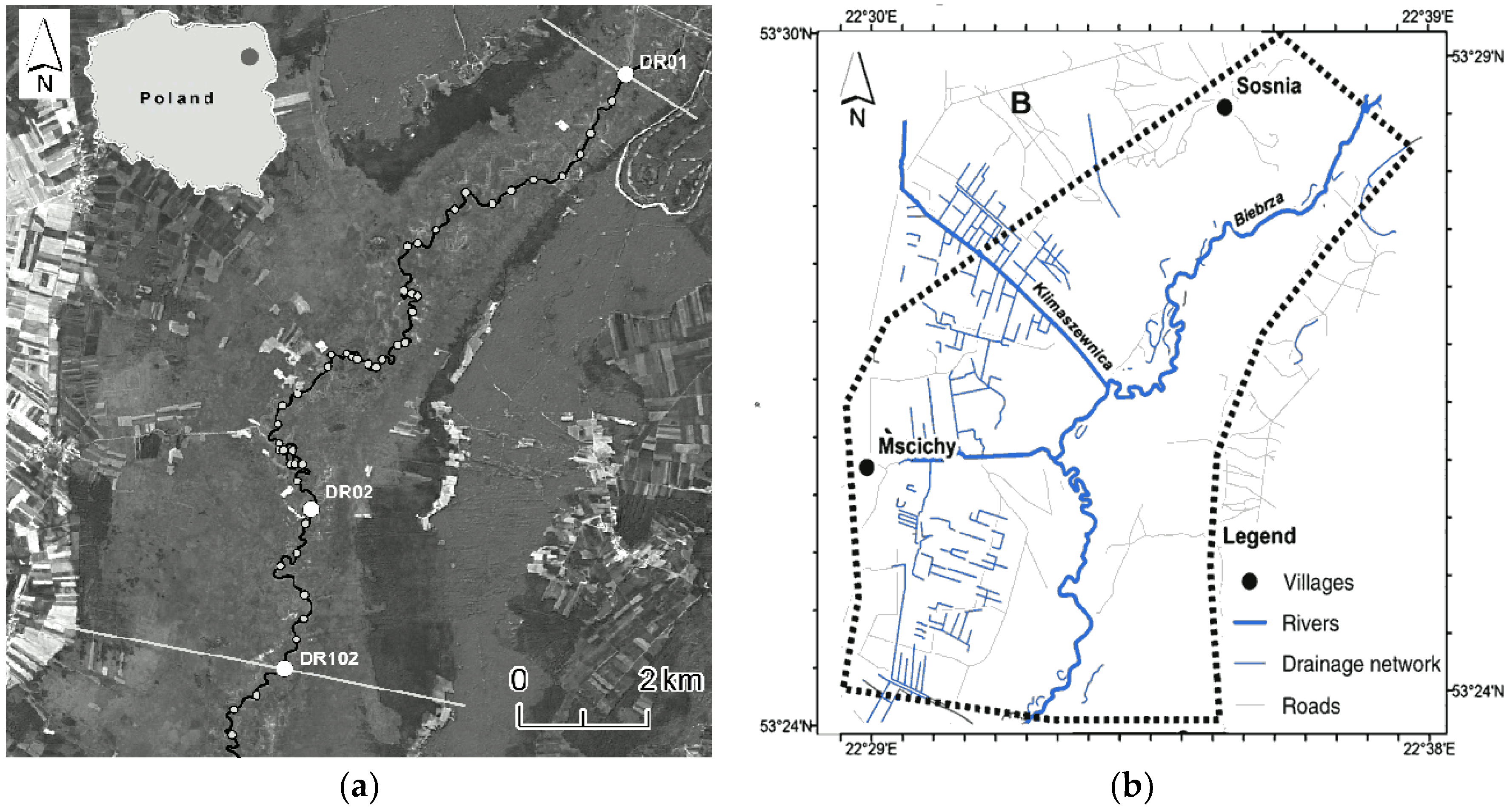
2.1. Study Area

The study area is situated in the northern part of the Lower Basin of the Biebrza Valley (Figure 1a), located in North-East Poland, becoming one of the most famous and ecologically valuable mosaics of riparian and mire ecosystems of Europe [39]. The analyzed area is a broad land depression that was formed in the late Pleistocene by fluvio-glacial waters of the Vistulian Glaciation. The valley is approximately 5 km wide and is filled with sand and covered with the peat soils of a maximal thickness of about 3 m, shaped in the Holocene. The length of the valley stretch reaches 12 km. Terrain elevations in the study area vary from 103 up to 118.5 m a.s.l. The Biebrza River is the main channel of the hydrodynamic network of the study area and it is about 18 km long, with an average bed slope close to 0.1‰ (Figure 1b). The river course winds and forms meanders, side streams, and old riverbeds which area activates only during periods of high water flows. The width of the river channel varies from 20 to 35 m. The river and floodplain feature in irregular cross sections and an irregular longitudinal profile [3]. An average discharge of the river Biebrza in the stretch analyzed reaches approximately 22.4 m³/s [40]. The average annual air temperature is equal to 6.6 °C [41] and the average annual sum of precipitation is as high as 560 mm [42]. The area is regularly flooded and the main source of water supply to wetlands of this part of the Biebrza Valley is flooding originating from the river Biebrza. The valley is densely vegetated by typical riparian plant and is covered by mosaic vegetation starting from sedge, sedge-moss, and reed communities to willow shrubs, black alder forest, swampy birch, and peat coniferous communities such as sedges, reed-manna grass, reeds, willow and alder shrubs, and forests [3,39,43]. River flooding which occurs regularly reinforces these representative water ecosystems every year. The majority of the study area is agriculturally managed as extensively used meadows of a seasonal mowing regime, but the vegetation remains near-natural. Additionally, the whole area analyzed is enclosed by the Natura 2000. The Biebrza Valley is known for its unique features as a migratory bird habitat and also as an ultimate area of protection of valuable and rare species of birds connected to wetlands [44]. The hydrodynamic models which describe the surface water flow in river and floodplain are a key tool in wetland management in the Biebrza Valley [3,45]. A particular challenge in the modeling process is to determine the effect of uncertainty of model elements on the quantitative description of hydrological factors, determining the proper functioning of wetland ecosystems. Our study contributes to the understanding of the impact of uncertainty of a floodplain digital terrain model on the 1D hydrodynamic flow calculation.

2.2. Digital Terrain Model (DTM)

The DTM used in this study for floodplain cross-sections and development of inundation maps was made by [46]. Below, a brief description of the model and applied methods is presented.

This is the high quality DTM, developed using novel methodology for the Biebrza River (Figure 1b). It was obtained using data from laser scanning, aerial and satellite imagery. It accounted for the land cover, identified using an object based image analysis of aerial and satellite images with spectral plant indices. Because of the vegetation, acquired terrain elevations were overestimated using standard processing methods for airborne scanning data [14,19,47]. A mean square error of the DTM would be close to 1 m. To improve the representation of the terrain, [46] introduced the altitude classes of vegetation (i.e., grasses, shrubs, reed), for which, on the basis of GPS measurements, it was possible to determine correction factors. The use of the object classification allowed for the separation of vegetation classes in areas overgrown by dense reeds and bushes. In those areas performing field measurements was not possible due to the lack of GPS signals or access. The determination of correction factors led to the introduction of adjustments regarding the altitude for the DTM. In areas with dense reeds and shrubs methods based on extrapolation and interpolation of terrain elevations were used.

A mean square error of the DTM, corrected in the respect to the vegetation classes, was twice smaller (0.5 m) than that obtained using only airborne scanning data.

2.3. 1D Hydrodynamic River and Floodplain Flow Model

The river and floodplain flow calculations were performed with a 1D model that is based on St. Venant equations with the friction law described by the Manning formula [48]. The ‘inertia terms’ in the momentum equation were neglected in the model. It was possible, as in the analyzed part of the Biebrza River the flow rate is relatively small (maximum river flow velocity is less than 0.4 m/s, the floodplain flow velocity does not exceed 0.1 m/s in a peak of flood events), changes in the stream velocity along the river reach are moderate and flood wave is slowly rising. When this simplification is made and the water level h is a dependent variable, the river flow can be explained using the equation of ‘diffusive wave approximation’. The diffusion wave approach may be preferred in simulations of the flood peaks in rivers and on floodplains with milder slopes that changes between 0.001 and 0.0001 (here 0.0001) and slowly increasing discharge [48,49,50,51].

The model was used for the flood wave modeling, recorded for the period between 11 November 2006 and 12 May 2007 in the analyzed river reach. The upstream boundary condition was defined for the upstream cross section, as the discharge hydrograph. For the downstream boundary condition at the DR102, the measured water level slope (0.00015) for a normal depth was applied (in both cases it was a Dirichlet condition). A downstream boundary condition can have an impact on the model sensitivity to the DTM uncertainty, therefore the river reach in its closest neighborhood—4 km upstream—has been excluded from the analysis. In the model, the inflow from the subcatchment has been estimated from discharge balances for the Burzyn gauge, located in the distance of 50 km from the upstream cross-section in the model and where observations have been performed by the Polish hydrological service. In the model the flow area is described by 59 river and floodplain cross-sections with an average distance of 250 m. Roughness coefficients used in the Manning’s formula are assigned according to the 1D model developed by Mirosław-Świątek [52] and are calibrated by “trial and error”. Results of the calculations are analyzed referring to the water level hydrograph recorded in the field, in the location of the automatic sensor, recording water levels, at a distance of 10 km from the first upstream cross-section (Figure 1). The calibrated Manning coefficient oscillated between 0.035 and 0.042 m^−1/3 s in the river channel, and from 0.055 to 0.11 m^−1/3 s on the floodplain.

Table 1. Model errors; MSE denotes Mean Squared Error, σ standard deviation, R correlation coefficient, h_max maximum water level, h_min minimum water level.

Variable	Sensor	Model
MSE (m)		0.05
σ (m)		0.02
R		0.971
hmax (m)	105.88	105.89
hmin (m)	105.30	105.22
dh = hmax − hmin (m)	0.67	0.58

presents model errors calculated for an automatic sensor. The range of changes in predicted water table elevations for a sensor location is within 12% of sensor readings, although the mean squared error (MSE) is 0.05 m. The value of the correlation coefficient R is 0.971 and standard deviation differences of water stages between calculated by a model and recorded by an automatic sensor is 0.02 m. It can be noted, that the model provides a good explanation of high water levels and poorer for low flows.

2.4. Sampling the DTM Uncertainty

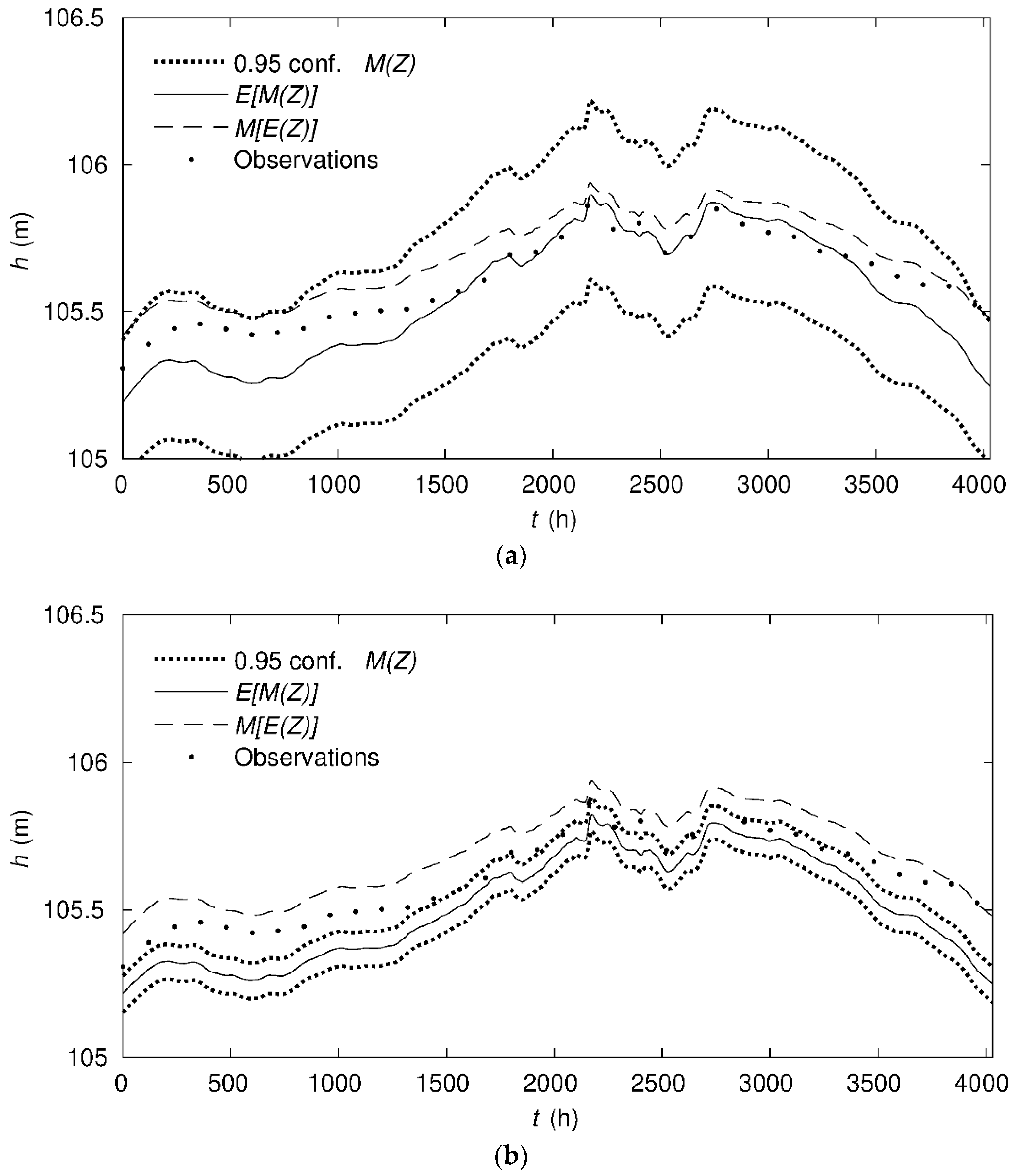
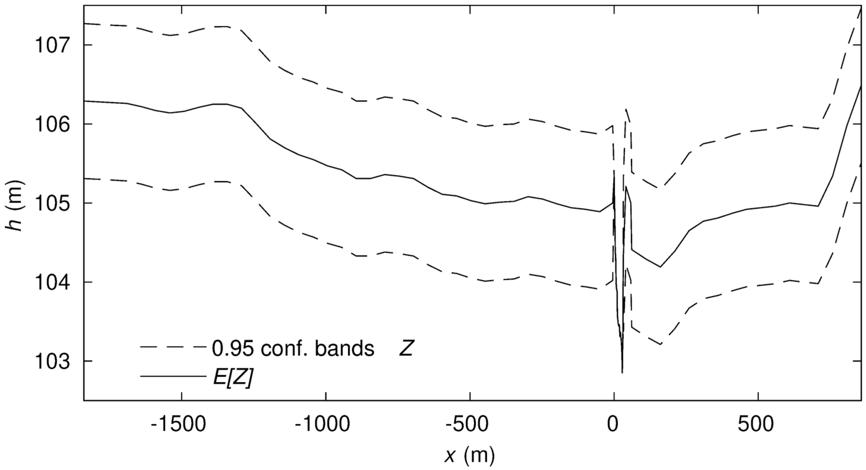
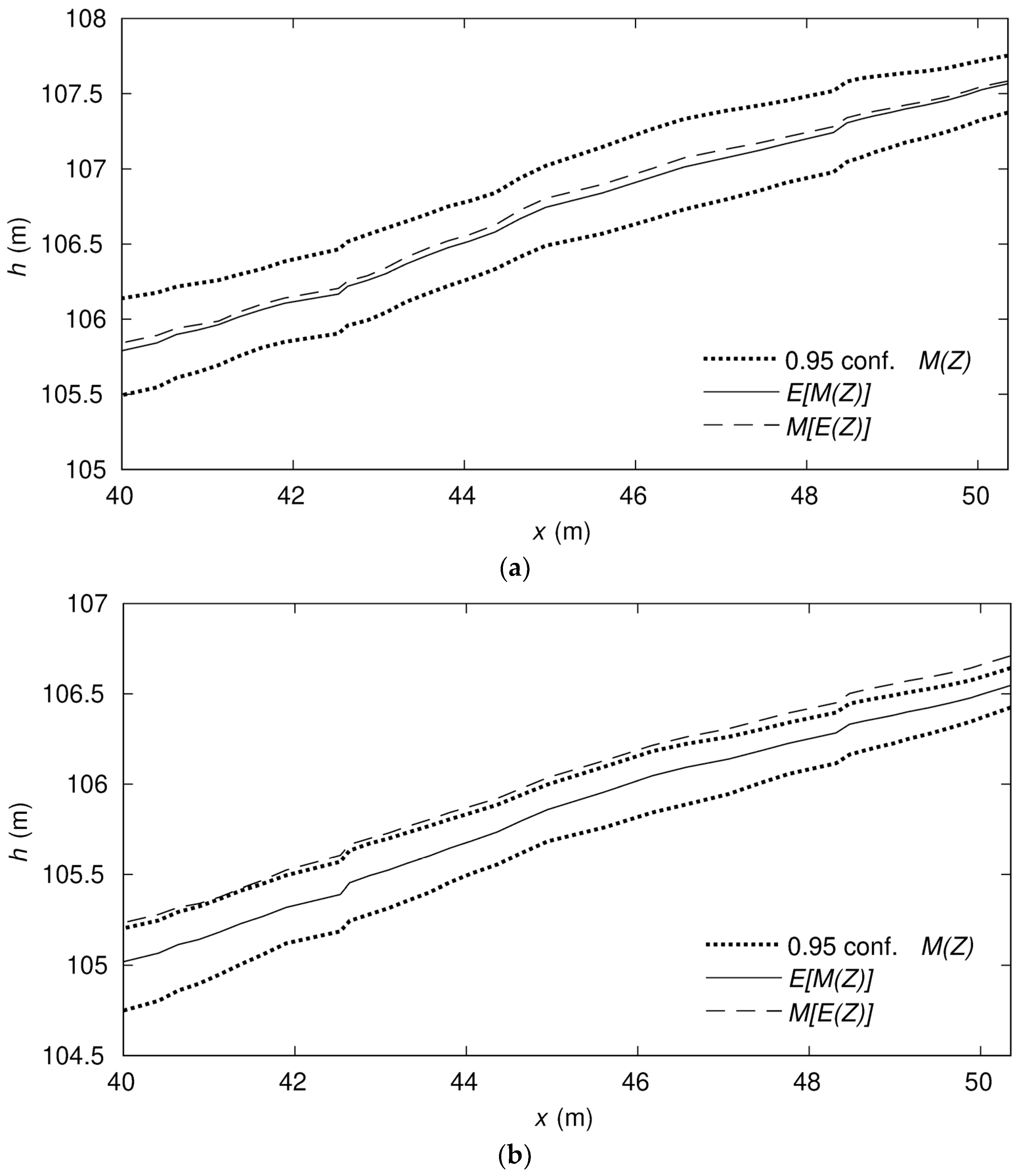
The methodology used for the development of the DTM has not yet provided grounds for an error model. Therefore, uncertainty of DTM was reproduced indirectly, assuming that it follows a normal distribution with a zero mean and a covariance estimated using DTM residuals and a correlation of elevation points [33,35]. The geometry representation in the 1D flow routing model is reduced to functions of a flow area and hydraulic radius, derived from the cross-sections. Because water strongly absorbs the visible light spectrum, the LIDAR scanning is useful only for the floodplain mapping [53]. Channel elevations have to be acquired directly using for example GPS measurements and it is expected that the resulting error is not significant for the hydraulic modeling. Therefore, it was assumed that the DTM uncertainty affects only floodplain parts of the cross-section. Floodplain elevations can be given then as:

$$Z=\widehat{Z}+\mathrm{e}$$

(1)

where $Z$ (m) denotes the vector of all elevation points, $\widehat{Z}$ (m) the nominal values, and $\mathrm{e}\sim N\left(0,\Sigma \right)$ (m) the noise, where $\Sigma$ stands for the $N\times N$ covariance matrix, with $N$ standing for the total number of elevation points in $Z$. The covariance matrix used to define the DEM uncertainty model depends on various factors, like land use and data processing techniques [14]. It can be estimated directly on the basis of a known structure of a DTM spatial error, assessed using extensive field measurements, which are rarely available. In the present study an indirect method was adopted. It was assumed that that the correlation of the elevation errors should follow the spatial correlation of elevations [33,35]. Then, the covariance matrix can be estimated on the basis of spatial correlation of elevations (correlogram) and RMSE of the DTM [32,54]. To reduce computational costs, the spatial correlation was estimated for cross-section points, extracted from the DTM. As the distance between cross-sections is considerably greater than between cross-section points, it was assumed that errors of elevation points are correlated only within a single cross-section. The elevation correlation longitudinal to the river flow was therefore neglected and the covariance between points of different cross-sections was given as zero. Non-zero values of the covariance matrix $\Sigma$ were computed on the basis of the spatial correlogram $C\left(d\right)$ [54], specifying the correlation between elevation points in a function of a distance $d$ (m). Therefore, the covariance matrix was determined for single $j$ cross section nodes $N_j$, rather than for $N$ all points. It can be obtained by multiplying the correlation coefficient by a fixed variation of elevations ${\sigma }^2$.

To analyze the significance of the spatial correlation on the flow modeling, the DTM uncertainty was also modeled assuming that errors in Equation (1) are uncorrelated $e\sim N\left(0,{\sigma }^2\right)$. The transformation of the DTM uncertainty through the hydraulic model was assessed using the Monte Carlo technique as in other geostatistical studies [17,31]. Water levels were calculated for the ensemble of cross-section elevation points, according to the Equation (1).

The impact of the DTM uncertainty on the computed water levels was analyzed in terms of the sample variation and a shift of the expected value from nominal one, obtained neglecting the DTM uncertainty. The first enables elaborating confidence limits of the computed water levels. The second allows investigating, how expected water levels are affected by uncertainty. The common assumption is that the input uncertainty has only an impact on the output variation and an expected value of the solution that includes uncertainty is the same as this evaluated for the nominal-expected input:

$$E\left[M\left(Z\right)\right]=M\left(E\left[Z\right]\right)$$

(2)

where $M\left(Z\right)$ denotes the model output for the uncertain elevations of the cross-section points $Z=\left\{Z_{1,1}{,Z}_{2,1},\dots \right\}$, $E\left[ \cdot \right]$ the expectation operator. With the noise $e\sim N\left(0,\Sigma \right)$ or $e\sim N\left(0,{\sigma }^2\right)$ (Equation (1)) the expected cross section elevations are the same as their nominal values: $E\left[Z\right]=\widehat{Z}$.

For nonlinear models Equation (2) does not necessarily hold true, this was demonstrated in a case of an uncertainty introduced to a flow model with roughness parameters [37,38,55,56,57].

3. Results

The standard deviation σ of a terrain elevation was estimated on the basis of the DTM model error that is approximately 0.50 m. The correlogram, an empirical correlation between points at a given cross section distance $d$ was computed using all cross section points. To obtain a uniform distance between points, to determine the correlation coefficient at a given distance, a linear interpolation was applied. The spatial correlation $C\left(d\right)$ used to generate the covariance matrix was obtained by fitting a spline function, using a Matlab framework of the Shape Language Modeling (SLM) provided by D’Errico [58] to the empirical correlation. To ensure that dependency will be positively semidefinite, the SLM fit is constrained, in such a way that the first derivative is negative: $C\prime \left(d\right)<0$. The correlogram indicated that at the distance of 1000 m the point correlation was about 0.81, and remaining above 0.7 up to 2000 m. Such high spatial correlation results from large uniform areas of the Biebrza valley. It also agrees with the expected uncertainty structure of the DTM—the elevation error for a given area, usually with similar vegetation, has a rather systematic nature—it should be constant for the whole zone [19].

The size of the Monte Carlo sample was estimated to ensure that the solution had converged (i.e., additional simulations do not affect the solution). For the uncertainty model accounting for the point correlation, the sample of 5000 combinations of cross section elevations is sufficient, while for the uncorrelated set, a significantly larger ensemble of 20,000 is necessary. The distribution of elevations for the cross section is given in Figure 2 in a form of the nominal values and 2.5% and 97.5% quantiles. Note, that the 95% elevation variability bands are the same for the correlated and uncorrelated samples.

For each set the water levels along the river reach were elaborated using a flood routing model. The solution in a form of calculated water levels that includes uncertainty has a probabilistic form. Such results are given here in a form of expected values: $E\left[M\left(Z\right)\right]$ and 95% confidence intervals. Results where the DTM uncertainty is disregarded, for the deterministic solution, are marked as $M\left(E\left[Z\right]\right)$.

In Figure 3 water levels obtained with (a) and without (b) DTM uncertainty are given for the cross section with observed water levels. Firstly, it can be noticed that the deterministic solution $M\left(E\left[Z\right]\right)$, the same for the correlated and uncorrelated DTM uncertainty, does not follow the probabilistic one $E\left[M\left(Z\right)\right]$. While for maximum water levels both solutions are relatively close, noticeable differences are present at lower water stages, where the deterministic solution agrees with the upper quantile of the probabilistic one. No matter whether it is based on the correlated or uncorrelated DTM uncertainty model, the expected values of probabilistic solutions provide a better fit with the observations, than a deterministic approach. Accounting for the elevation uncertainty allowed to improve the explanation of low flows, maintaining a good agreement with observation for high flows. It can be also noticed that the mean water levels are underestimated by approximately 5 cm when the uncertainty correlation is neglected, compared to the correlated case.

Confidence bands of the water levels for the uncorrelated DTM uncertainty are narrow comparing to those obtained for the correlated input. However, these narrow bands seem to be too optimistic, as observations at lower stages went beyond their span. Much wider bands for the correlated DTM uncertainty fully enclose the observations. It can be also noticed, that the standard deviation of the water levels for the correlated set is very close to the assumed standard deviation of elevations. For the uncorrelated set it is almost three times smaller.

Figure 4 shows water levels along the river reach for maximum (a) and bankfull flows (b), with the correlated DTM errors. As in the case of Figure 3 the expected value of the solution that includes the uncertainty $E\left[M\left(Z\right)\right]$ is very close to the deterministic one $M\left(E\left[Z\right]\right)$, with a difference noticeable bellow 0.10 m. This is not a case for bankfull flows, where the discrepancy is much higher, exceeding 0.2 m. The results for the uncorrelated sample of elevations follows a similar pattern but with much more narrow confidence bands and higher water levels for near bankfull flows.

The discrepancies between deterministic and probabilistic approaches are much more significant, if water levels are being used to estimate inundation extents. The computed inundation areas are provided in

Table 2. The effect of elevation uncertainty on calculated inundation areas for high and near bankfull flows.

Variable	Bankfull Flows			Maximum Flows
	Corr. DTM Unc.	Uncorr. DTM Unc.	Determ. Solution	Corr. DTM Unc.	Uncorr. DTM Unc.	Determ. Solution
A2.5% (106 m2)	1.83	2.90	7.75	22.33	23.38	25.28
E[A] (106 m2)	3.12	3.81		24.33	23.75
A97.5% (106 m2)	4.70	4.75		25.62	24.12

Corr. Stands for correlated, Uncorr. uncorrelated, unc. uncertainty, determ. deterministic.

and inundation extent for maximum flows is showed in Figure 5. In delineation of inundations, the effect of the elevation uncertainty in the extent mapping was neglected, investigating only the uncertainty of computed water levels. The confidence intervals A_2.5%, A_97.5% and expected values E[A] were obtained directly on the basis of calculated inundation extents for each Monte Carlo sample [37]. Inundation extents were computed for maximum flows and for the lowest flows at which inundation appears—Close to bankfull flows. The presented values allow for much better interpretation of differences in water levels between different approaches. For near bankfull flows, it resulted in more than the 100% higher estimate of inundation extent for the deterministic solution than for the expected value of the probabilistic one. It is interesting that the upper confidence band for the correlated set is below the uncorrelated, despite the fact that it was opposite in the case of water levels. This comes from the strong nonlinearity introduced through inundation delineation. The model sensitivity on the elevation uncertainty in respect of the inundation extent is much smaller for high flows with differences below 5%.

To explain the differences in deterministic and probabilistic approaches, the effect of the elevation uncertainty on the parametrization of the cross section geometry was also investigated. Calculations in the 1D hydraulic models are based on functions representing geometric properties of the cross section. The most significant is the relationship between the hydraulic radius and water levels. Figure 6 presents the hydraulic radius obtained with and without the DTM uncertainty for the sections of the compound cross section. Results are provided for the correlated (a–c) and uncorrelated (d–f) DTM uncertainties at a chosen cross section. Uncertainty affects only the hydraulic radius above the river banks, approximately at 1.3 m, as elevations of the main channel (Figure 6a,d) were not acquired from the DTM. The highest discrepancies between values computed with and without the DTM uncertainty are present just above the river banks, what can be seen for the hydraulic radius for floodplains (Figure 6b,c,e,f). This is a region where the wetted perimeter is high in relation to the flow area, what makes the hydraulic radius very sensitive to the elevation fluctuations. This might be an explanation for much higher differences between the probabilistic and deterministic solutions at lower water stages.

Figure 6, also shows the difference in the response of the hydraulic radius to the correlation of the elevation points. It is apparent that narrow confidence bands for water levels obtained for the DTM uncertainty model without correlation result from small variability of the hydraulic radius, much smaller than when the DTM elevation errors are correlated. It is also interesting that the median of hydraulic for the correlated DTM uncertainty is much closer to one obtained from undisrupted elevations. The correlation term in the uncertainty model allows to maintain initial shape of the cross section.

The explanation of a high sensitivity of the hydraulic model on the elevations uncertainty for bankfull flows and moderate for flood flows seems to be straightforward. The noise term applied to the elevations affects the wetted perimeter and flow area. Their variability is much higher for uncorrelated distortions, when elevations can independently vary. The effect is noticeable for low flows with a relatively small flow area and affected with the elevation uncertainty—at bankfull depths. For high flows, variations of the wetted perimeter become less significant due to a larger flow area.

4. Discussion

The propagation of the DTM uncertainty in flood routing, especially for 1D models is rarely analyzed. The case study of Biebrza River shows that it has a noticeable effect on computed water levels. For the approach that accounted for the DTM uncertainty correlation, the standard deviation of calculated water levels is almost the same as deviation of DTM elevations. For case studies such as the analyzed river reach, with relatively high DTM errors, the output uncertainty might have noticeable effect on further derivatives, as discussed in [9]. On the other hand, following the study of [26], for river reaches with less developed vegetation, effects will be noticeable smaller. It is interesting that high variation in water levels does have a very strong impact on maximum inundation extents. This supports the outcomes of [37], showing the similar effect for flood extents computed in the respect to the total model uncertainty. Still, however, as reported by [27], estimated inundation extents with uncertainty are slightly below those obtained neglecting it.

The uncertainty of computed water levels and inundation extents, depends on the spatial correlation of DTM uncertainties. Neglecting the spatial correlation, results in much smaller variation in flow model outputs and also a lower estimate of maximum water levels. It contradicts the assumption of [30] that neglecting the spatial correlation of the uncertainty can be considered as ‘the worst case scenario’. Therefore, as it is suggested by [17,31] DTM uncertainty should be analyzed along with its spatial dependency, at least in the case of 1D models.

The 1D model appears to be the most sensitive to the correlation of the DTM uncertainty near bankfull flows. It is demonstrated on the basis of computed inundation extents. The uncorrelated elevation distortions in cross section elevations, introduced when the DTM uncertainty is neglected, affects the shape of the cross section parametrization in the form of the hydraulic radius. The effect decreases for higher flows, when elevation distortion becomes small in the respect to the flow area. This might suggest, that the choice of DTM uncertainty model might be less crucial in flood assessment studies.

It should be also noted, that the response of 1D model for the DTM uncertainty is different, as in the case of 2D approaches, as in the first case it does not affect the discretization of the flow field. In 2D cases [27,28] the model uncertainty have an effect on a computational domain, that might result in a change of the flow direction, impossible in the case of 1D models.

The interesting finding of the study is that accounting for the elevation uncertainty significantly improves the model explanation of water levels. The deterministic approach, in which uncertainty was neglected, leads to an overestimation of lower flows. Including uncertainty with the correlation, it allows improvement of the model explanation of the process, as the observations were enclosed within confidence bands. The demonstrated improvement of the model explanation of the water levels, when the DTM uncertainty with correlation, is included, suggests that it could be possible to narrow confidence bands of flood routing models. The presented approach could be potentially useful in studies on flow conditions of rivers with densely vegetated floodplains. In such cases, the modeling output can be significantly affected by the elevation uncertainty. Accounting for it should allow obtaining a more accurate representation of a river system. However, the significance and joint effects of the DTM uncertainty with respect to other sources of the uncertainty like parametrization of hydraulic roughness remain open questions, which require further studies.

References

1. Gharbi, M.; Soualmia, A.; Dartus, D.; Masbernat, L. Comparison of 1D and 2D hydraulic models for floods simulation on the medjerda riverin tunisia. J. Mater. Environ. Sci. 2016, 7, 3017–3026. [Google Scholar]
2. Grygoruk, M.; Bańkowska, A.; Jabłońska, E.; Janauer, G.A.; Kubrak, J.; Mirosław-Światek, D.; Kotowski, W. Assessing habitat exposure to eutrophication in restored wetlands: Model-supported ex-ante approach to rewetting drained mires. J. Environ. Manag. 2015, 152, 230–240. [Google Scholar] [CrossRef] [PubMed]
3. Świątek, D.; Szporak, S.; Chormański, J.; Okruszko, T. Hydrodynamic model of the lower biebrza river flow a tool for assessing the hydrologic vulnerability of a floodplain to management practices. Ecohydrol. Hydrobiol. 2008, 8, 331–337. [Google Scholar] [CrossRef]
4. Marcinkowski, P.; Kiczko, A.; Okruszko, T. Model-based analysis of macrophytes role in the flow distribution in the anastomosing river system. Water 2018, 10, 953. [Google Scholar] [CrossRef]
5. Brandyk, A.; Majewski, G.; Kiczko, A.; Boczoń, A.; Wróbel, M.; Porretta-Tomaszewska, P. Ground water levels of a developing wetland—Implications for water management goals. In Environmental Engineering V, Proceedings of the 5th National Congress of Environmental Engineering, Lublin, Poland, 29 May–1 June 2016; CRC Press: Boca Raton, FL, USA, 2017. [Google Scholar]
6. Li, Z.; Zhu, C.; Gold, C. Digital Terrain Modeling: Principles and Methodology; CRC press: Boca Raton, FL, USA, 2004; ISBN 9780203486740. [Google Scholar]
7. Sanders, B.F. Evaluation of on-line DEMs for flood inundation modeling. Adv. Water Resour. 2007, 30, 1831–1843. [Google Scholar] [CrossRef]
8. Teng, J.; Jakeman, A.J.; Vaze, J.; Croke, B.F.W.; Dutta, D.; Kim, S. Flood inundation modelling: A review of methods, recent advances and uncertainty analysis. Environ. Model. Softw. 2017, 90, 201–216. [Google Scholar] [CrossRef]
9. Mirosław-Świątek, D.; Kiczko, A.; Szporak-Wasilewska, S.; Grygoruk, M. Too wet and too dry? Uncertainty of DEM as a potential source of significant errors in a model-based water level assessment in riparian and mire ecosystems. Wetl. Ecol. Manag. 2017, 25, 547–562. [Google Scholar] [CrossRef] [Green Version]
10. Walczak, Z.; Sojka, M.; Wrózyński, R.; Laks, I. Estimation of polder retention capacity based on ASTER, SRTM and LIDAR DEMs: The case of Majdany Polder (West Poland). Water 2016, 8, 230. [Google Scholar] [CrossRef]
11. Reutebuch, S.E.; McGaughey, R.J.; Andersen, H.-E.; Carson, W.W. Accuracy of a high-resolution LIDAR terrain model under a conifer forest canopy. Can. J. Remote Sens. 2003, 29, 527–535. [Google Scholar] [CrossRef]
12. Sofia, G.; Pirotti, F.; Tarolli, P. Variations in multiscale curvature distribution and signatures of LIDAR DTM errors. Earth Surf. Process. Landf. 2013, 38, 1116–1134. [Google Scholar] [CrossRef]
13. Liu, X.; Hu, P.; Hu, H.; Sherba, J. Approximation theory applied to DEM vertical accuracy assessment. Trans. GIS 2012, 16, 397–410. [Google Scholar] [CrossRef]
14. Hodgson, M.E.; Jensen, J.R.; Schmidt, L.; Schill, S.; Davis, B. An evaluation of LIDAR-and IFSAR-derived digital elevation models in leaf-on conditions with USGS Level 1 and Level 2 DEMs. Remote Sens. Environ. 2003, 84, 295–308. [Google Scholar] [CrossRef]
15. Hodgson, M.E.; Bresnahan, P. Accuracy of airborne LIDAR-derived elevation. Photogramm. Eng. Remote Sens. 2004, 70, 331–339. [Google Scholar] [CrossRef]
16. Raber, G.T.; Jensen, J.R.; Hodgson, M.E.; Tullis, J.A.; Davis, B.A.; Berglund, J. Impact of LIDAR nominal post-spacing on DEM accuracy and flood zone delineation. Photogramm. Eng. Remote Sens. 2007, 73, 793–804. [Google Scholar] [CrossRef]
17. Oksanen, J.; Sarjakoski, T. Uncovering the statistical and spatial characteristics of fine toposcale DEM error. Int. J. Geogr. Inf. Sci. 2006, 20, 345–369. [Google Scholar] [CrossRef]
18. Guo, Q.; Li, W.; Yu, H.; Alvarez, O. Effects of topographic variability and lidar sampling density on several DEM interpolation methods. Photogramm. Eng. Remote Sens. 2010, 76, 701–712. [Google Scholar] [CrossRef]
19. Aguilar, F.J.; Mills, J.P.; Delgado, J.; Aguilar, M.A.; Negreiros, J.G.; Pérez, J.L. Modelling vertical error in LiDAR-derived digital elevation models. ISPRS J. Photogramm. Remote Sens. 2010, 65, 103–110. [Google Scholar] [CrossRef]
20. Merwade, V.; Olivera, F.; Arabi, M.; Edleman, S. Uncertainty in flood inundation mapping: Current issues and future directions. J. Hydrol. Eng. 2008, 13, 608–620. [Google Scholar] [CrossRef]
21. Papaioannou, G.; Loukas, A.; Vasiliades, L.; Aronica, G.T. Flood inundation mapping sensitivity to riverine spatial resolution and modelling approach. Nat. Hazards 2016, 83, 117–132. [Google Scholar] [CrossRef]
22. Papaioannou, G.; Vasiliades, L.; Loukas, A.; Aronica, G.T. Probabilistic flood inundation mapping at ungauged streams due to roughness coefficient uncertainty in hydraulic modelling. Adv. Geosci. 2017, 44, 23–34. [Google Scholar] [CrossRef] [Green Version]
23. Laks, I.; Sojka, M.; Walczak, Z.; Wróżyński, R. Possibilities of using low quality digital elevation models of floodplains in hydraulic numerical models. Water 2017, 9, 283. [Google Scholar] [CrossRef]
24. Yan, K.; Di Baldassarre, G.; Solomatine, D.P. Exploring the potential of SRTM topographic data for flood inundation modelling under uncertainty. J. Hydroinform. 2013, 15, 849–861. [Google Scholar] [CrossRef]
25. Podhoranyi, M.; Fedorcak, D. Inaccuracy introduced by LIDAR-generated cross sections and its impact on 1D hydrodynamic simulations. Environ. Earth Sci. 2015, 73, 1–11. [Google Scholar] [CrossRef]
26. Jung, Y.; Merwade, V. Uncertainty quantification in flood inundation mapping using generalized likelihood uncertainty estimate and sensitivity analysis. J. Hydrol. Eng. 2012, 17, 507–520. [Google Scholar] [CrossRef]
27. Tsubaki, R.; Kawahara, Y. The uncertainty of local flow parameters during inundation flow over complex topographies with elevation errors. J. Hydrol. 2013, 486, 71–87. [Google Scholar] [CrossRef]
28. Abily, M.; Bertrand, N.; Delestre, O.; Gourbesville, P.; Duluc, C.M. Spatial global sensitivity analysis of high resolution classified topographic data use in 2D urban flood modelling. Environ. Model. Softw. 2016, 77, 183–195. [Google Scholar] [CrossRef] [Green Version]
29. Knighton, J. Estimating the effects of DEM uncertainty through two-dimensional spatial stochastic watershed simulation. In Proceedings of the World Environmental and Water Resources Congress 2015, Austin, TX, USA, 17–21 May 2015; pp. 1489–1499. [Google Scholar]
30. Heuvelink, G.B.M. Error Propagation in Environmental Modelling with GIS; CRC Press: Boca Raton, FL, USA, 1998. [Google Scholar]
31. Oksanen, J.; Sarjakoski, T. Error propagation of DEM-based surface derivatives. Comput. Geosci. 2005, 31, 1015–1027. [Google Scholar] [CrossRef]
32. Wechsler, S.P. Uncertainties associated with digital elevation models for hydrologic applications: A review. Hydrol. Earth Syst. Sci. 2007, 11, 1481–1500. [Google Scholar] [CrossRef]
33. Hengl, T.; Heuvelink, G.B.M.; Van Loon, E.E. On the uncertainty of stream networks derived from elevation data: The error propagation approach. Hydrol. Earth Syst. Sci. 2010, 14, 1153–1165. [Google Scholar] [CrossRef]
34. Oksanen, J. Digital Elevation Model Error in Terrain Analysis. Ph.D. Thesis, University of Helsinki, Helsinki, Finland, 2006. [Google Scholar]
35. Lewis, A.; Hutchinson, M.F. From Data Accuracy to Data Quality: Using Spatial Statistics to Predict the Implications of Spatial Error in Point Data; Ann Arbor Press: Chelsea, MI, USA, 2000. [Google Scholar]
36. Kozioł, A.P.; Kubrak, J. Measurements of turbulence structure in a compound channel. In Rivers—Physical, Fluvial and Environmental Processes; Springer: Berlin, Germany, 2015; pp. 229–254. [Google Scholar]
37. Romanowicz, R.J.J.; Kiczko, A. An event simulation approach to the assessment of flood level frequencies: Risk maps for the Warsaw reach of the River Vistula. Hydrol. Process. 2016, 30, 2451–2462. [Google Scholar] [CrossRef]
38. Kiczko, A.; Romanowicz, R.J.; Osuch, M.; Karamuz, E. Maximising the usefulness of flood risk assessment for the river Vistula in Warsaw. Nat. Hazards Earth Syst. Sci. 2013, 13, 3443–3455. [Google Scholar] [CrossRef]
39. Wassen, M.J.; Okruszko, T.; Kardel, I.; Chormański, J.; Światek, D.; Mioduszewski, W.; Bleuten, W.; Querner, E.P.; El Kahloun, M.; Batelaan, O.; et al. Eco-hydrological functioning of the Biebrza wetlands: Lessons for the conservation and restoration of deteriorated wetlands. In Wetlands: Functioning, Biodiversity Conservation, and Restoration; Springer: Berlin, Germany, 2006; pp. 285–310. [Google Scholar]
40. Grygoruk, M.; Batelaan, O.; Okruszko, T.; Mirosław-Świątek, D.; Chormański, J.; Rycharski, M. Groundwater modelling and hydrological system analysis of wetlands in the Middle Biebrza Basin. In Modelling of Hydrological Processes in the Narew Catchment; Springer: Berlin, Germany, 2011; pp. 89–109. [Google Scholar]
41. Banaszuk, H. Ogolna charakterystyka Kotliny Biebrzańskiej i Biebrzańskiego Parku Narodowego [General characteristics of the Biebrza Valley and the Biebrza National Park]. In Kotlina Biebrzańska i Biebrzański Park Narodowy. Aktualny stan, walory, zagrożenia i potrzeby czynnej ochrony środowiska. Monografia przyrodnicza [The Biebrza Valley and the Biebrza National Park. Current State, Natural Values, Threats and Needs]; Wyd. Ekonomia i Środowisko: Białystok, Poland, 2004; pp. 19–25. [Google Scholar]
42. Kossowska-Cezak, U. Climate of the Biebrza ice-margin Halley. Pol. Ecol. Stud. 1984, 10, 253–270. [Google Scholar]
43. Oświt, J. Roślinność i Siedliska Zabagnionych Dolin Rzecznych na tle Warunków Wodnych. [Vegetation and Wetland Habitats against the Background of Water Conditions]; Wydawnictwo Naukowe PWN: Warsaw, Poland, 1991; ISBN 83-01-10396-5. [Google Scholar]
44. Maciorowski, G.; Mirski Pawełand Kardel, I.; Stelmaszczyk, M.; Mirosław-Swiatek, D.; Chormański, J.; Okruszko, T. Water regime as a key factor differentiating habitats of spotted eagles Aquila clanga and Aquila pomarina in Biebrza Valley (NE Poland). Bird Study 2015, 62, 120–125. [Google Scholar] [CrossRef]
45. Chormański, J.; Mirosław-Świaątek, D.; Michałowski, R. A hydrodynamic model coupled with GIS for flood characteristics analysis in the Biebrza riparian wetland. Oceanol. Hydrobiol. Stud. 2009, 38, 65–73. [Google Scholar] [CrossRef]
46. Mirosław-Świątek, D.; Szporak-Wasilewska, S.; Michałowski, R.; Kardel, I.; Grygoruk, M. Developing an algorithm for enhancement of a digital terrain model for a densely vegetated floodplain wetland. J. Appl. Remote Sens. 2016, 10. [Google Scholar] [CrossRef]
47. Gorte, B.; Pfeifer, N.; Elberink, S.O. Height texture of low vegetation in airborne laser scanner data and its potential for DTM correction. Int. Arch. Photogramm. Remote Sens. Spat. Inf. Sci. 2005, 36, 150–155. [Google Scholar]
48. Miroslaw-Swiatek, D.; Grygoruk, M. Influence of equivalent flow path approximation in 1D model in meandering rivers with floodplain on flood routing. In Proceedings of the 15th International Multidisciplinary Scientific GeoConference SGEM 2015, Albena, Bulgaria, 18–24 June 2015; pp. 379–386. [Google Scholar]
49. Ponce, V.M.; Simons, D.B.; Li, R.-M. Applicability of kinematic and diffusion models. J. Hydraul. Div. 1978, 104, 353–360. [Google Scholar]
50. Weinmann, B.P.E.; Laurenson, E.M. Approximate Flood Routing Methods: A Review. J. Hydraul. Div. 1979, 105, 1521–1536. [Google Scholar]
51. Kazezyılmaz-Alhan, C.M. An improved solution for diffusion waves to overland flow. Appl. Math. Model. 2012, 36, 4165–4172. [Google Scholar] [CrossRef]
52. Mirosław-Świątek, D. Application of Newtonian nudging data assimilation method in hydrodynamic model of flood flow in the Lower Biebrza Basin. Stud. Geotech. Mech. 2012, 34, 91–105. [Google Scholar] [CrossRef]
53. Pe’eri, S.; Philpot, W. Increasing the existence of very shallow-water LIDAR measurements using the red-channel waveforms. IEEE Trans. Geosci. Remote Sens. 2007. [Google Scholar] [CrossRef]
54. Bjørnstad, O.N.; Falck, W. Nonparametric spatial covariance functions: Estimation and testing. Environ. Ecol. Stat. 2001, 8, 53–70. [Google Scholar] [CrossRef]
55. Kiczko, A.; Szelag, B.; Koziol, A.P.; Krukowski, M.; Kubrak, E.; Kubrak, J.; Romanowicz, R.J. Optimal capacity of a stormwater reservoir for flood peak reduction. J. Hydrol. Eng. 2018, 23. [Google Scholar] [CrossRef]
56. Brandyk, A.; Kiczko, A.; Majewski, G.; Kleniewska, M.; Krukowski, M. Uncertainty of Deardorff’s soil moisture model based on continuous TDR measurements for sandy loam soil. J. Hydrol. Hydromech. 2016, 64, 23–29. [Google Scholar] [CrossRef] [Green Version]
57. Szelag, B.; Kiczko, A.; Dabek, L. Sensitivity and uncertainty analysis of hydrodynamic model (SWMM) for storm water runoff forecasting in an urban basin—A case study. Ochrona Srodowiska 2016, 38, 15–22. [Google Scholar]
58. D’Errico, J. SLM Shape Language Modeling; MathWorks: Natick, MA, USA, 2016. [Google Scholar]
59. OpenStreetMap. Available online: www.openstreetmap.org (accessed on 18 August 2018).
Figure 1. Study area. (a) Northern stretch of the Lower Biebrza Valley, starting at the cross-section DR01 and ending at DR102, DR02 denotes the localization of the automatic sensor (observation point), locations of remaining cross-sections are marked with dots [46]; (b) Northern part of the Lower Basin of the Biebrza with dashed lines showing Digital Terrain Model (DTM) area.
Water 10 01308 g001
Figure 2. Cross section next the measurement point with elevation uncertainty; x denotes cross section width; h elevation a.s.l.
Water 10 01308 g002
Figure 3. Computed water levels with and without uncertainty during a freshet for the cross-section next to the measurement point. The E[M(θ)] stands for the expected output of the probabilistic model enclosed by 0.95 confidence intervals, M[E(θ)] is for the deterministic model, and dots for observations; (a) for the correlated DTM uncertainty; (b) for uncorrelated.
Water 10 01308 g003
Figure 4. Water levels along the river reach for the correlated elevation uncertainty (a) high flows (b) bankfull flows.
Water 10 01308 g004
Figure 5. Probability map of inundation extent as the result of correlated DTM uncertainty; the red dashed line indicate the solution neglecting the DTM uncertainty; base map was developed using OpenStreetMap layers [59].
Water 10 01308 g005
Figure 6. The hydraulic radius computed with and without the uncertainty for the cross-section next to the measurement point; (a–c) for the correlated DTM uncertainty; (d–f) for uncorrelated; RMCh (a or d), denotes hydraulic radius for the main channel, RLFP (b or e) and RRFP (c or f) for the left and right floodplain, respectively.
Water 10 01308 g006