Optimal Allocation of Water Resources from the “Wide-Mild Water Shortage” Perspective

Abstract

A major objective of the optimization of water resources allocation is to ensure the supply an adequate amount of water to users at the right time and maximize the utilization of water resources. However, in case of insufficient water supply, water shortage is likely to occur intensively for specific water users or in specific periods, referred to as a “concentrated water shortage”. The risk of a concentrated water shortage should be shared across a wider range of users and periods, so that it would have a less severe impact on each calculation unit in each period, which we refer to as the “wide-mild water shortage”. In this study, the nonlinear weight of the water supply objective function can be converted into a piecewise linear weight based on the law of diminishing marginal utility, making it possible to reduce or even eliminate the concentrated water shortage and thus making the allocation of water resources more reasonable. The case study in the Nen River basin in northeast China shows that the improved method results in a significant increase in water shortage units but a significant reduction in water shortage range. As a consequence, water shortage is more uniformly distributed from April to June, which contributes to solving the concentrated water shortage problem in May. However, it should be noted that to what extent the wide-mild water shortage can be realized depends not only on the marginal utility of water demand, but also on the available water supply and the regulative capacity of water supply projects. In spite of this, the improved method enables water to be supplied more suitably for users at the appropriate time, which contributes to improving the utilization of water resources and helping decision-makers better address the problem of concentrated water shortage.

1. Introduction

Rapid industrialization and urbanization in China have led to a growing demand for water resources for domestic, agricultural, industrial, and ecological purposes in recent years, making the optimal allocation of water resources an important, challenging task. With better understanding of real-world problems, advancing data availability and reliability, researchers are committed to developing large-scale and complex water resources allocation models, and to developing effective algorithms for solving the allocation models [1]. Commonly used methods for the optimization of medium- and long-term water resource allocation include dynamic programming, linear programming, and nonlinear programming [2,3]. However, in order to solve an optimization problem using dynamic programming, the principles of optimality and non-aftereffect must both be satisfied [4]. Dynamic programming may also suffer from the curse of dimensionality in solving complex water resources allocation problems in which the storage demands and complexity costs grow exponentially with the dimension of the state space. Nonlinear programming is useful in solving optimization problems where some of the constraints or the objective function are nonlinear [5] and difficult to be linearized [6], or a large error may arise from linearization. However, it is important to note that nonlinear programming may not always converge on the global optimal solution. Linear programming has the advantages of easy modeling, easy availability of necessary parameters, and convergence to the global optimal solution. Obviously, linear programming is preferred to solve medium- and long-term water resource allocation problems [7,8,9,10,11,12,13,14,15].

The linear programming method has been used to solve the allocation of water resources in the Mahanadi River in northeastern India, in which the seasonal unit-price of surface water or groundwater can be taken as the objective function weights [16]. When the available water is insufficient to meet all the agricultural water demand, the optimization result may cause the occurrence of concentrated water shortages in a certain period due to the lower unit-price in agriculture than that in other users. Even if more water has been supplied for agriculture in the early period, zero full water costing [17] will be presented resulting in no crop harvest due to a seriously concentrated water shortage. A water economy optimization model has been developed by Mirchi in South Florida to quantitatively weigh water management priorities [18]. A characteristic of the penalty function, which is only determined by the relative magnitude by investigation and analysis, is that the function itself has no practical significance. An interval multi-objective programming model has been established to optimize the irrigation water allocation in Hulan River in China [19]. The interval function, which was solved by linear programming, was used as the weight of the objective function. The max–min operator [20] is used to solve the maximum and minimum of the interval function by generalization as a linear or nonlinear function. If the interval function is generalized as a nonlinear function, the solution method is the same as the nonlinear programming. If the interval function is generalized as a linear function, the assumption is that the marginal utility function is linear and inconsistent with the actual curve. Furthermore, economic benefit/utility [21,22,23], ecological flow [24], soil moisture uniformity and yield [25], maximization of economic, ecological, and social benefits [26], and investment, operation, and environmental costs [27] can also be taken as the objective function weights and solved by linear programming.

Nevertheless, it is noteworthy that all the above weights used to maximize the total water supply benefit or minimize the loss resulting from water shortage are derived under the assumption that the benefit yield of every unit water supply is the same, regardless of the satisfaction level of the water demand. Obviously, this assumption does not hold given the law of diminishing marginal utility. As a consequence, what appears to be theoretically optimal may not be feasible in practical settings. Brown et al. [28,29] showed that, in some cases, the marginal utility of insufficient instream flows was considerably higher than that of the water consumption of users. For these seasons, it is necessary to take into account the law of diminishing marginal utility in water resources allocation.

Suppose there are n agricultural plots along the water channel in an irrigation district, which are denoted as i = 1, 2, …, n from the channel head to its terminal end, and the effective utilization coefficient of irrigated water follows the order of ${\eta }_1>{\eta }_2>\dots \dots >{\eta }_n$ due to the impact of transport distance and water loss. All plots are assumed to have the same soil properties and are planted with the same crop species. The water demand benefit per unit area, as well as the benefit per unit water use ${\lambda }_i$, is the same, and thus the average benefit per unit water use at different periods is also the same. Thus, the total water demand of the irrigation district is the sum of the water demand of each plot ($W_{real\_d}={\displaystyle \sum _{i=1}^n{W}_{i,net}/{\eta }_i}$). If the objective is to maximize the total irrigation benefit and water supply is allocated according to ${\lambda }_i$, the programming is a linear problem. Thus, if the available water supply is higher than or equal to the total water demand $W_{real\_d}$, the water demands of all plots can be well satisfied; whereas, in the case of insufficient water supply, the water demands of plots can be satisfied in order from the channel head to the terminal end until the supply of water is exhausted. In this circumstance, water shortage is likely to occur in plots at the terminal end at any time, which is referred to as a “concentrated water shortage” in this study due to the optimization rules. It is important to note that if crop fails due to an extremely low supply of water in a specific period, then the actual benefit of previous periods is equal to 0. This problem is rarely taken into account in most previous models. For large-scale water resources systems responsible for supplying water from multiple sources to multiple users in multiple periods via multiple water supply channels, the allocation scheme based on the benefit per unit water use rather than on the marginal utility may easily result in the occurrence of concentrated water shortage.

Generally, there are two kinds of concepts about water shortages, which are “concentrated water shortage” and “wide-mild water shortage”. Concentrated water shortage refers to dense water shortage occurring in specific water users or periods, which is not affected by the precipitation and water demand. Wide-mild water shortage, the antonym of concentrated water shortage, refers to the occurrence of relatively uniform water shortage in a specific period or a specific domain. Similar to the “strategic” and “tactical” water resources allocation problems mentioned by Turgeon [30], concentrated water shortage is “strategic” and wide-mild water shortage is “tactical”.

The optimization results based on concentrated water shortage are often unrealistic, and sometimes very bad, which will have a direct impact on people’s trust and application. In order to overcome this problem, the constraints of minimum water supply are added to the water demand of each calculation unit in each period.

However, given the balance conditions between water demand and water supply in each calculation unit, it is very difficult to define the constraints of the minimum water supply in a long series of inflows. Too low constraints may not solve the problem of concentrated water shortage; while constraints that are too high may be infeasible for optimization. Accordingly, the objective of this study is to solve the nonlinear water resources allocation problem using the linear programming based on the rule of diminishing marginal utility, and this study may provide a simple but effective way for the optimization of water resources allocation.

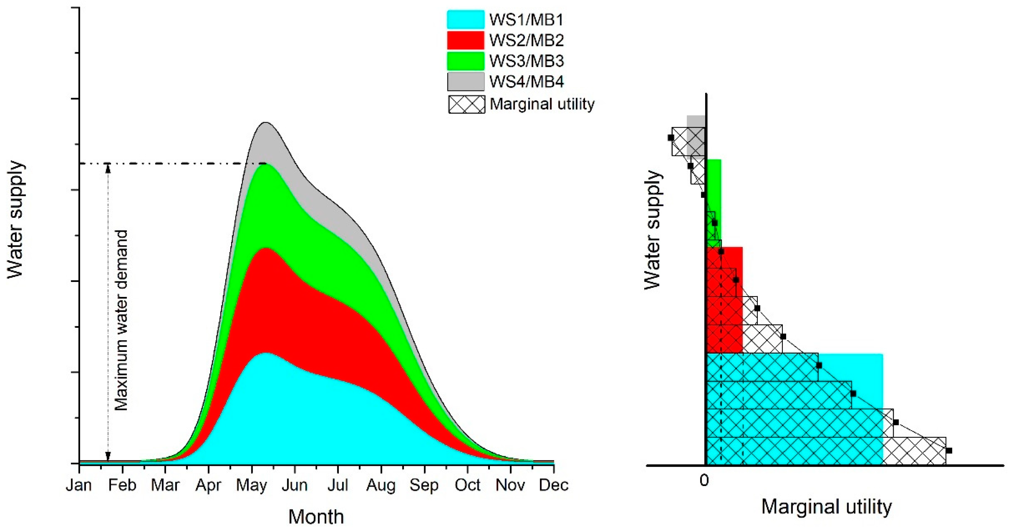
2. Diminishing Marginal Utility in Water Resources Utilization

The concept that the marginal utility of each homogenous unit decreases as the supply of units increases (and vice versa), provided that other conditions are the same, is referred to as the “law of diminishing marginal utility”. This law has been widely recognized as the explanation of numerous economic phenomena in the field of economics, and exists in reality including its application to the water resources field. For example, Figure 1 shows the agricultural water supply benefit and its marginal utility. In water deficient northeast China, deficit irrigation makes it possible to save more water for other purposes or to irrigate more land. On the contrary, excessive irrigation may cause waterlogging and consequently the reduction of crop yield. It is evident that the law of diminishing marginal utility should be considered in order to ensure the allocation of water resources to be more realistic and effective.

3. Water Resources Optimal Allocation from the Perspective of “Wide-Mild Water Shortage”

3.1. The Concept of Wide-Mild Water Shortage

The law of diminishing marginal utility is explicitly neglected in current methods for the optimization of water resources allocation based on benefit per unit water use, which can easily cause the occurrence of concentrated water shortage. As a consequence, (a) the theoretically optimal scheme may not be optimal in practice; (b) a concentrated water shortage that occurs in a specific period may result in a significant benefit/loss not only in this period, but also in earlier and later periods; and (c) given the complex interactions among different water users, the sudden occurrence of a concentrated water shortage for one water user can also bring about a significant benefit/loss of other water users, such as hydroelectric power generation. Thus, in case of insufficient water supply, the risk of concentrated water shortage should be shared across calculation units, periods, and users. In doing so, more calculation units, periods, and users may suffer from water shortage, but the water shortage would have less severe impacts on each calculation unit in each period, which we refer to as the concept of “wide-mild water shortage”. The wide-mild water shortage is expected to be achieved by optimizing water resource allocation based on the law of diminishing marginal utility. Theoretically, such a problem is a nonlinear problem that can be solved by nonlinear programming. In fact, the optimization of water resources allocation is very complex, and linear programming, instead of the nonlinear programming, is often used in this context.

In this study, the nonlinear function is approximated by a piecewise linear function, in which the total water demand in each period is divided into piecewise water demands with different marginal utilities. The demands of different calculation units, periods, and users are optimized in the water resources system, and the rest are the same as that in the optimization of water resources allocation based on benefit per unit water use.

3.2. Piecewise Linear Function

For a complex water resources system, it is extremely difficult, if not impossible, to establish an accurate piecewise linear function specifically for each water demand in each unit, period, and user, and to accurately determine their marginal utilities and, very often, it is not necessary to do so. Although the allocation of water resources based on the benefit per unit water use may occasionally lead to concentrated water shortage that is unacceptable and, as stated before, the accuracy requirement can be well satisfied.

In order to determine the piecewise linear function and marginal utilities, it is important to (a) determine the rank of the average benefit for each water demand, which is the same as the optimization based on the benefit per unit water use; (b) determine the marginal utilities for different satisfaction levels of water demands and then divide them into piecewise segments according to the percentage of water demands. However, the number of piecewise segments should not be too large; (c) examine whether there is an overlap of marginal utilities among different water demands. A sufficiently high marginal utility should be set for those periods during which water shortage is not allowed, and the precision can be set to a level that would have no impact on optimization; (d) examine whether there is a difference in benefit of the same water demand in different calculation units. If a significant difference is found, they should be treated differently; otherwise they can be treated in the same way; and (e) analyze the relationship of the same water demand at different periods in a specific calculation unit. Piecewise segments can be obtained according to the percentage of water demands; however, adjustment can be made if necessary. Much effort has been made to better understand the water use benefit function, such as the Cobb–Douglas production function [31] and piecewise function [32,33], which are not described in detail herein.

3.3. Methodology

The objective function for the optimization of water resources allocation based on the average benefit per unit water use (hereafter referred to as the “original method”) can be described as follows.

$$\begin{array}{l}MaxObj=Max[{\displaystyle \sum _{k=1}^{KN}{\displaystyle \sum _{t=1}^{TN}{\displaystyle \sum _{j=1}^{JN}B{L}_{k,t,j}}}}\times W{L}_{k,t,j}+{\displaystyle \sum _{r=1}^{RN}{\displaystyle \sum _{t=1}^{TN}{\displaystyle \sum _{h=1}^{HN}B{R}_{r,t,h}\times W{R}_{r,t,h}}}}]\end{array}$$

(1)

The major constraints concerning the water supply are as follows,

$$\begin{array}{l}W{L}_{k,t,j}\le DW{L}_{k,t,j}\end{array}$$

(2)

$$\begin{array}{l}W{R}_{r,t,h}\le DW{R}_{r,t,h}\end{array}$$

(3)

$$\begin{array}{l}W{L}_{k,t,j}={\displaystyle \sum _{i=1}^{IKJN}XW{L}_{k,t,j,i}}\end{array}$$

(4)

$$\begin{array}{l}W{R}_{r,t,h}={\displaystyle \sum _{i=1}^{IRHN}XW{R}_{r,t,h,i}}\end{array}$$

(5)

where Obj is the objective function; k is the sequence number of calculation units; KN is the total number of calculation units; t is the sequence number of periods in a year; TN is the total number of periods in a year and TN = 12 when the calculation is performed on a monthly basis; j is the sequence number of socioeconomic water use types, JN is the total number of socioeconomic water use types; r is the sequence number of rivers/lakes; RN is the total number of rivers/lakes; h is the sequence number of river/lake ecological flow types; HN is the total number of river/lake ecological flow types; i is the sequence number of water sources; IKJN is the total number of water sources for the water use type j in the calculation unit k; IRHN is the total number of water sources for the water use type h of river/lake r; $DW{L}_{k,t,j}$ is the water demand j in the calculation unit k; $XW{L}_{k,t,j,i}$ is the water supply from water source i to $DW{L}_{k,t,j}$; $W{L}_{k,t,j}$ is the total water supply from each water source to $DW{L}_{k,t,j}$; $DW{R}_{r,t,h}$ is the ecological water demand h of river/lake r; $XW{R}_{r,t,h,i}$ is the total water supply from water source i to $DW{R}_{h,t,r}$; $W{R}_{r,t,h}$ is the total water supply from each water source to $DW{R}_{r,t,h}$; $B{L}_{k,t,j}$ is the average benefit of $W{L}_{k,t,j}$ per unit water supply; and $B{R}_{r,t,h}$ is the average benefit of $W{R}_{r,t,h}$ per unit water supply, respectively.

The improved objective function based on the law of diminishing marginal utility (hereafter referred to as the “improved method”) is:

$$MaxObj=Max[{\displaystyle \sum _{k=1}^{KN}{\displaystyle \sum _{t=1}^{TN}{\displaystyle \sum _{j=1}^{JN}{\displaystyle \sum _{s=1}^{SJN}BL{S}_{k,t,j,s}}}}}\times WL{S}_{k,t,j,s}+{\displaystyle \sum _{r=1}^{RN}{\displaystyle \sum _{t=1}^{TN}{\displaystyle \sum _{h=1}^{HN}{\displaystyle \sum _{s=1}^{SHN}B}R{S}_{r,t,h,s}\times WR{S}_{r,t,h,s}}}}]$$

(6)

The following water demand constraints are considered.

$$DW{L}_{k,t,j}={\displaystyle \sum _S^{SKJN}DWL{S}_{k,t,j,s}}$$

(7)

$$DW{R}_{r,t,j}={\displaystyle \sum _S^{SRHN}DWR{S}_{r,t,h,s}}$$

(8)

Constraints in Equations (2)–(5) can be converted into Equations (9)–(12), respectively:

$$WL{S}_{k,t,j,s}\le DWL{S}_{k,t,j,s}$$

(9)

$$WR{S}_{r,t,h,s}\le DWR{S}_{r,t,h,s}$$

(10)

$$WL{S}_{k,t,j,s}={\displaystyle \sum _{i=1}^{IKJSN}XWL{S}_{k,t,j,s,i}}$$

(11)

$$WR{S}_{r,t,h,s}={\displaystyle \sum _{i=1}^{IRHSN}XW{R}_{r,t,h,s,i}}$$

(12)

where s is the piecewise number of a water demand, SKJN is the total piecewise number of water demand j in the calculation unit k, SRHN is the total piecewise number of water demand h of river/lake r, $DWL{S}_{k,t,j,s}$ is the socioeconomic water demand of the segment s for the water demand h in the calculation unit k, $DWR{S}_{r,t,h,s}$ is the ecological water demand of the segment s for the water demand j of river/lake r in the calculation unit t, $BL{S}_{r,t,j,s}$ is the marginal utility of the socioeconomic water demand of the segment s for the water demand j in the calculation unit k, $WL{S}_{k,t,j,s}$ is the water supply corresponding to the socioeconomic water demand, $BR{S}_{r,t,h,s}$ is the marginal utility of the ecological water demand of the segment s for river/lake r in the calculation period t, and $WR{S}_{r,t,h,s}$ is the water supply corresponding to the ecological water demand.

The diminishing marginal utility can be described as:

$$BL{S}_{k,t,j,1}>BL{S}_{k,t,j,2}>......>BL{S}_{k,t,j,SKJN}\forall k,t,j$$

(13)

$$BR{S}_{r,t,h,1}>BR{S}_{r,t,h,2}>......>BR{S}_{r,t,j,SRHN}\forall r,t,h$$

(14)

Accordingly, the agricultural water demand process is shown in Figure 2. The left figure is the piecewise of water demand. The blue, red, green, and gray areas stand for four piecewise segments. The total area of blue, red, and green is the water demand. The grey area represents excess water demand. The right figure is marginal utility curve (black curve). The black curve should be divided into piecewise segments of the corresponding water supply, shown as the black bar. The blue, red, green, and gray bars represent the average value of the black bar within the percentage of water demands: the closer to the bottom, the greater the marginal utility. The grey area of the water supply exceeds the maximum water demand so that its marginal utility is negative.

4. Case Study

4.1. Study Area

The Nen River basin is located in the northeast region of China and flows through Heilongjiang Province, Inner Mongolia and Jilin Provinces, China with a drainage area of 298,500 km². The average annual precipitation is 455 mm, the average annual and monthly precipitation of different frequency are shown in Figure 3. In 2013, the basin has a total population of 16.56 million with an urban population of 8.22 million, a gross domestic product (GDP) of 861.6 billion RMB, an industrial added value of 396.6 billion RMB, a total grain yield of 36.74 billion kilograms, and a livestock population of 25.2 million. It has an effective irrigation area of 2.5 million hectares, a forest and fruit growing area of 21.4 thousand hectares, and a grassland area of 4.5 thousand hectares. By the year 2013, the basin has 429 water supply projects with a total capacity of 16.0 billion m³ and an effective capacity of 10.4 billion m³. There are three main water resource zones called NEJ, JQ, and BST from upstream to downstream. The total water supply is 37.7 billion m³, with the surface water, groundwater, and recycled water accounting for 61.4%, 38.5%, and 0.1%, respectively. The main crops cultivated in the Nen River basin include rice, corn, wheat, and soybean. Sowing often begins in early or middle April, and the water demand reaches a peak 40–80 days after seeding (approximately from May to August). The agricultural water demand accounts for approximately 74% of the total water demand in the basin. However, the runoff peak occurs from July to September, indicating that the precipitation, runoff, and agricultural water demand are not temporally concurrent (see Figure 4). The most pronounced imbalance between water supply and demand is observed in May, resulting in the highest probability of severe water shortage.

In this study, the water related information including water resources, economy and ecosystem of the Nen River basin are simplified into nodes (water resources projects, control sections, and calculation units) and lines (channels, rivers, etc.) [34], and the resulted water resources allocation network chart is shown in Appendix Figure A1. The system consists of 47 calculation units, 33 reservoirs, 48 river and channel nodes, 161 water supply channels, water release channels, and river channels. The water is supplied mainly for urban domestic use, rural domestic use, irrigation, industrial use, urban ecological environment, river, and lake ecological environment, etc. The water sources include surface water, groundwater, and recycled water from urban sewage. The calculation is done on a monthly basis. The monthly runoff data for the period 1956–2013 and the monthly water demand data of the current year (2013) and the planning year (2020) are collected and analyzed.

4.2. Parameter Determination

The model inputs include water demands, water sources, water resources projects, operational constraints, water resources allocation system, benefits of various water demands, etc. The runoff, allowable exploitation quantity of groundwater, and parameters of water resources projects (mainly including water storage, division, pumping, and transfer projects), and channel parameters can be obtained by survey (see Appendix

Table A1. Engineering parameters.

Name	Catchment Area km2	Flood Control Capacity Million m3	Storage Capacity Million m3	Dead Capacity Million m3
BR1	66,382	8610	6456.3	487.5
BR2	3745	995	740	310
BR3	683	117	74	7
BR4	1660	281	162	14
BR5	15,112	260	177	23
BR6	2241	298	49	5
BR7	13,500	150	84	14
BR8	/	450	315	110
BR9	7780	1253	1067	34
BR10	548	235	207	63.5
BR11	342	51	40.6	4
BR12	60	209	390.3	34.5
BR13	35	110	107	10
BR14	5300	405	405	105
PR1	8250	1685	1483	320
PR2	10,720	989	859	242
PR3	24,384	/	350	50
PR4	32,229	3331	3507	1007
PR5	19,487	3113	2554	556
PR6	16,137	3508	2926	248
PR7	1990	187	143	32
PR8	2050	754	754	95
PR9	2072	307	132	45
PR10	438	70	31	1
PR11	853	96	43.64	6.33
PR12	1773.6	240	220	104
PR13	2444	450	380	132
PR14	8200	3100	3100	1455
PR15	12,426	1640	1486	198
PR16	1790	538.2	352	19.4
PR17	4206	76	45	8
PR18	7610	574	498	31
PR19	9050	360	132	86

”/” indicates that the information is not known.

). However, it is difficult to obtain the benefit information of various water demands. In this study, the average benefit of each water demand can be obtained by survey and statistics, and then the marginal utilities for different satisfaction levels of water demand are obtained by analysis of typical examples and expert discussion. The applicability of each typical benefit function for the water demand in different calculation units is rated by experts [35]. The benefits of urban, river, and lake ecological environment are not available in statistics. Thus, the relative importance or benefit per unit water use for different water users is rated by experts, and then the average benefits and marginal utilities are determined. According to the precision requirements and the difficulty in determining the marginal utilities, the water demand for each water user is divided into three segments, and thus only three marginal utility values need to be determined in this study.

5. Results and Discussion

In this study, we only discuss the water supply and shortage quantity obtained by the original and improved methods in the planning year of 2020.

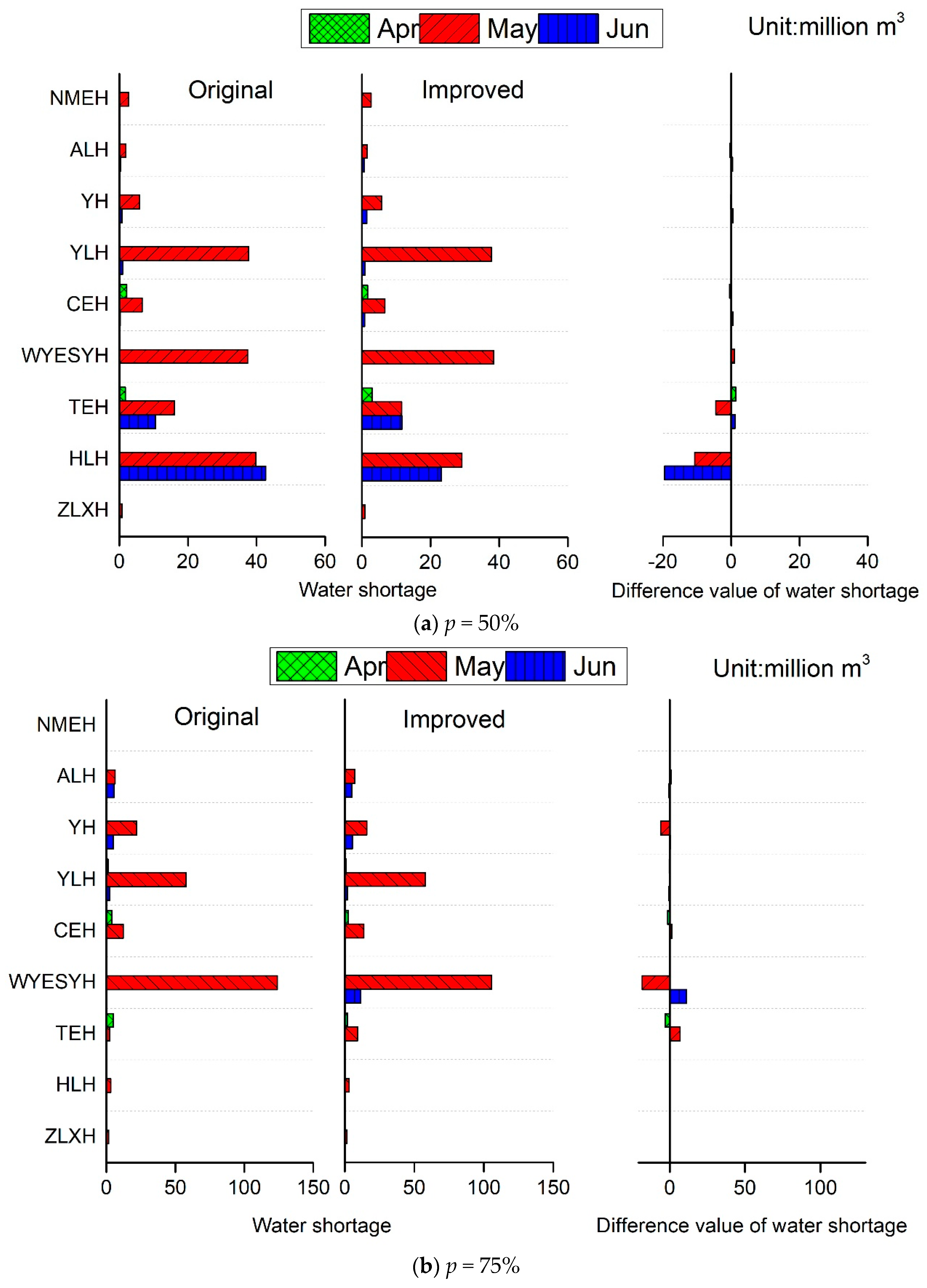
5.1. Water Supply and Shortage

Before model improvement, the water supply of NEJ, JQ, and BST (see Appendix

Table A2. Basic information about water resource zones

Water Resource Zone	Catchment Area km2	Water Use (in 2013) Billion m3	Sub Units
NEJ	67,775	0.36	GGHRUP/GH/GGHR TONEJR
JQ	99,678	4.82	NMH/NMEH/NER TOTH/ALH/YH/YLH/TH TO JQ
BST	131,049	7.43	CEH/THE/HLH/JQ TO BST/BST TO SHJ/WYESYH/AZXH/ZLXH

) were 0.93 billion cubic meters, 6.62 billion cubic meters, and 24.18 billion cubic meters, respectively. After model improvement, their respective water supplies were 0.93 billion cubic meters, 6.61 billion cubic meters, and 24.17 billion cubic meters, with little change.

Before model improvement, water shortages of NEJ, JQ, and BST regions totaled 0 billion cubic meters, 0.22 billion cubic meters, and 0.33 billion cubic meters, respectively. After model improvement, they totaled 0 billion cubic meters, 0.23 billion cubic meters, and 0.33 billion cubic meters, respectively, with little change. Among all domains, agricultural water shortage is still the highest.

Obviously, water supply will not change due to the model improvement.

5.2. Changes in the Units with Water Shortage

The water resource allocation in 47 calculation units of four primary water users during a 58-year period (1956–2013) in the Nen River basin was optimized (a total of 130,848 sets of data), and

Table 1. Changes in the units with agricultural water shortage before and after model improvement.

Precipitation Frequency	Model	Numerator *	Denominator #	Ratio (%)
p = 50%	Before improvement	492	74448	0.66
	After improvement	853		1.15
p = 75%	Before improvement	205	29328	0.70
	After improvement	285		0.97
p = 90%	Before improvement	90	27072	0.33
	After improvement	192		0.71
Total	Before improvement	787	130848	0.60
	After improvement	1330		1.02

* Numerator = Number of years in a given precipitation frequency× Number of calculation units with water shortage in the specific years × Number of users × Number of months in one year. ^# Denominator = Total number of years (mentioned above) × Number of calculation units × Number of users × Number of months in one year.

shows the changes in total number of units with water shortage before and after model improvement under different precipitation frequency conditions. Clearly, the number of units with water shortage increases in the improved model, all of which are related to agricultural water shortage.

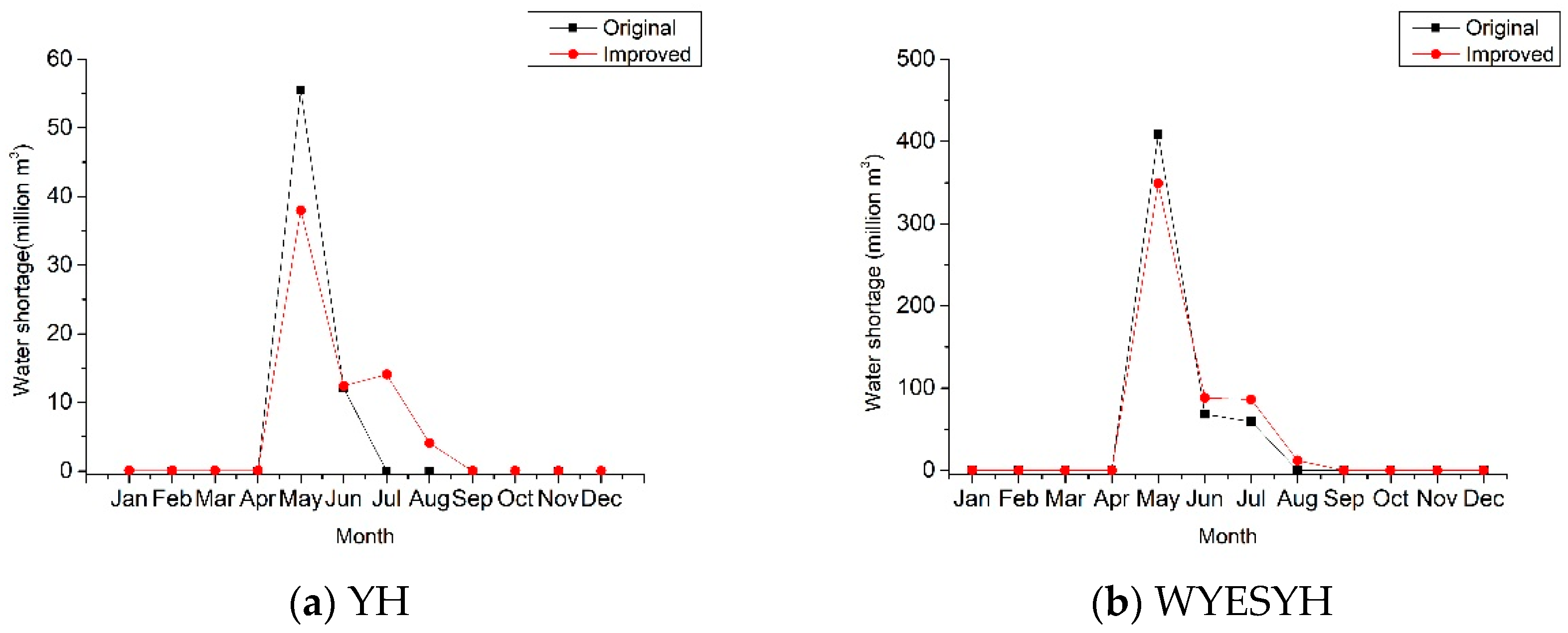
5.3. Comparison of Water Shortage and Process

The water demand for irrigation reaches a peak in the 40-day ponding period from early April to middle/late May in the Nen River basin; the water consumption for irrigation accounts for approximately 1/6 of the total annual water consumption. However, precipitation is low in April on average, accounting for only 3.3% of the total annual precipitation. The most pronounced imbalance between water supply and demand is observed in April, resulting in the highest probability of severe water shortage. Figure 5 shows changes in water shortage and the difference in the value of water shortage of nine units from April to June before and after model improvement. The differences in water storage quantity in May obtained by original and improved methods (red bars) vary substantially and are predominantly negative; whereas that in April (green bars) and June (blue bars) are mostly positive. In addition, the water shortage quantity increases significantly in June under a precipitation frequency of 75% and 90%. It can be concluded that the improved method results in wide-mild water shortage from April to June, which contributes to solving the concentrated water shortage problem and the imbalance between inflow and water supply from April to June.

Figure 6 and Figure 7 show the comparison of monthly water shortage for two typical units (YH and WYESYH, the most water shortage areas in Nen River basin) obtained by original and improved methods at a precipitation frequency of 75% and 90%, respectively. Clearly, the improved method results in a wide-mild distribution of the water shortage for YH and WYESYH in May at a 75% precipitation frequency, indicating a significant improvement of the concentrated water shortage. The similar results are also obtained at a 90% precipitation frequency, and the water shortage becomes less severe in June and July. However, a more obvious decrease in the peak of water shortage is obtained at a precipitation frequency of 75% than 90%.

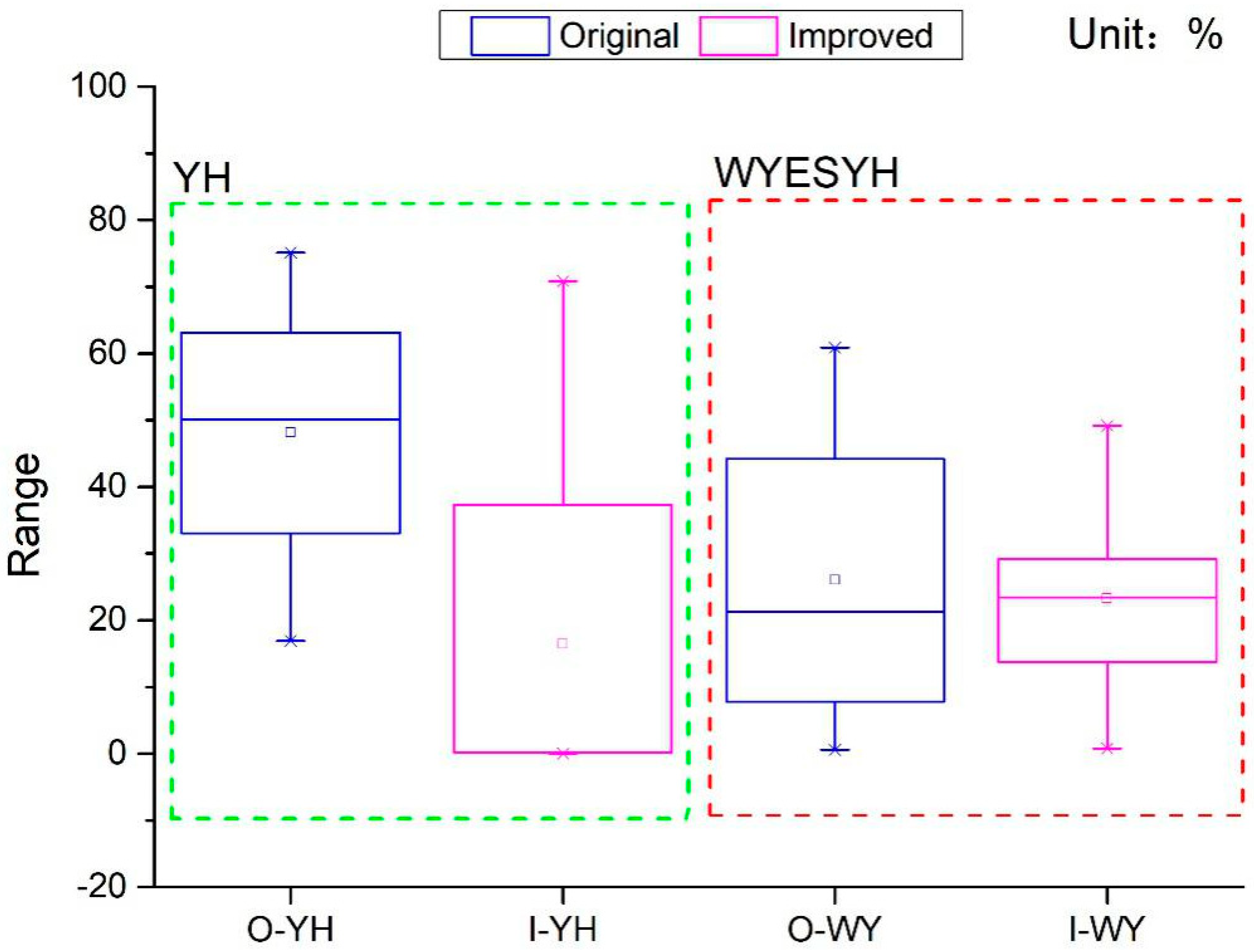
5.4. Comparison of Water Shortage Range

Figure 8 shows the comparison of the average annual water shortage range, minimum water shortage range (except 0), and maximum water shortage range obtained by the original and improved methods. It shows that despite the significant increase in the number of water shortage units, the water shortage range is reduced, which may give the false impression that the original method could obtain more satisfactory results. However, the high probability of concentrated water shortage in a specific period (i.e., the peak water demand period in irrigation) is largely ignored in the original operation, which may consequently lead to benefit loss. After the improvement, the problem of large water shortage range can be well-solved, making the optimization operation more acceptable.

Figure 9 and Figure 10 show changes in water shortage range for the two units (YH and WYESYH) according to the monthly average water shortage and maximum water shortage. Obviously, after improvement, the water shortage range is obviously reduced, indicating that the water demand can be better satisfied by the improved method proposed in this study.

6. Conclusions

In this study, the “wide-mild water shortage” perspective is proposed based on the law of diminishing marginal utility in order to solve the problem of concentrated water shortage. We argue that the risk of concentrated water shortage should be shared across a wider range of users and periods, so that it would have less severe impacts on each individual user in each period. It is necessary to redefine the weight of variables in the water supply objective function. Assuming that the weight is a continuous nonlinear function, and can be converted into a piecewise linear weight, it is possible to reduce or even eliminate the concentrated water shortage, thus making the allocation of water resources more reasonable.

The case study was carried out in the Nen River Basin, northeast China and shows that the improved method results in a significant increase in water shortage units, but a significant reduction in the water shortage range. As a consequence, the water shortage is more uniformly distributed from April to June, which contributes to solving the concentrated water shortage problem and the mismatch between inflow and water supply from April to June. However, it should be noted that the extent to which the wide-mild water shortage can be realized depends, not only on the marginal utility of water demand, but also on the available water supply and the capacity of water supply projects. In spite of this, the improved method enables the water to be supplied more uniformly at the appropriate time, which contributes to improving the allocation efficacy of water resources and helps decision-makers better deal with the problem of concentrated water shortages.

References

1. Cai, X.; McKenney, D.C.; Lasdon, L.S.; Watkins, D. Solving large nonconvex water resources management models using generalized benders decomposition. Oper. Res. 2001, 49, 235–245. [Google Scholar] [CrossRef]
2. Bradley, S.; Hax, A.; Magnanti, T. Applied Mathematical Programming; Addison Wesley: Boston, MA, USA, 1977. [Google Scholar]
3. Singh, A. An overview of the optimization modelling applications. J. Hydrol. 2012, 466–467, 167–182. [Google Scholar] [CrossRef]
4. Powell, W.B. Approximate Dynamic Programming: Solving the Curses of Dimensionality; Wiley & Sons: Hoboken, NJ, USA, 2011. [Google Scholar]
5. Luenberger, D.G.; Ye, Y.Y. Linear and Nonlinear Programming, 3rd ed.; Springer: Berlin, Germany, 2008. [Google Scholar]
6. Li, M.; Fu, Q.; Singh, V.P.; Ma, M.; Liu, X. An intuitionistic fuzzy multi-objective non-linear programming model for sustainable irrigation water allocation under the combination of dry and wet conditions. J. Hydrol. 2017, 555, 80–94. [Google Scholar] [CrossRef]
7. Lu, H.W.; Huang, G.H.; He, L. Development of an interval-valued fuzzy linear-programming method based on infinite α-cuts for water resources management. Environ. Model. Softw. 2010, 25, 354–361. [Google Scholar] [CrossRef]
8. Fu, Y.; Li, M.; Guo, P. Optimal allocation of water resources model for different growth stages of crops under uncertainty. J. Irrig. Drain. Eng. 2014, 140, 1272–1273. [Google Scholar] [CrossRef]
9. Li, M.; Guo, P.; Zhang, L.; Zhao, J. Multi-dimensional critical regulation control modes and water optimal allocation for irrigation system in the middle reaches of Heihe River basin, China. Ecol. Eng. 2015, 76, 166–177. [Google Scholar] [CrossRef]
10. Yang, L.; Liu, S.; Tsoka, S.; Papageorgiou, L.G. Mathematical programming for piecewise linear regression analysis. Exp. Syst. Appl. 2016, 44, 156–167. [Google Scholar] [CrossRef] [Green Version]
11. Zhang, C.L.; Guo, P. A generalized fuzzy credibility-constrained linear fractional programming approach for optimal irrigation water allocation under uncertainty. J. Hydrol. 2017, 553, 735–749. [Google Scholar] [CrossRef]
12. Hong, X.D.; Liao, Z.W.; Jiang, B.B.; Wang, J.D.; Yang, Y.R. Targeting of heat integrated water allocation networks by one-step MILP formulation. Appl. Energy 2017, 197, 254–269. [Google Scholar] [CrossRef]
13. Bettinger, P.; Boston, K.; Siry, J.P.; Grebner, D.L. Forest Management and Planning Chapter 7—Linear-Programming; Academic Press: Cambridge, MA, USA, 2017; pp. 153–176. [Google Scholar]
14. Eiger, G.; Shamir, U.; Ben-Tal, A. Optimal design of water distribution networks. Water Resour. Res. 1994, 30, 2637–2646. [Google Scholar] [CrossRef]
15. Li, D.; Haimes, Y.Y. Optimal maintenance-related decision making for deteriorating water distribution system 2: Multilevel decomposition approach. Water Resour. Res. 1991, 28, 1063–1070. [Google Scholar] [CrossRef]
16. Das, B.; Singh, A.; Panda, S.N.; Yasuda, H. Optimal land and water resources allocation policies for sustainable irrigated agriculture. Land Use Policy 2015, 42, 527–537. [Google Scholar] [CrossRef]
17. Gonelas, K.; Kanakoudis, V. Reaching Economic Leakage Level through Pressure Management. Water Sci. Technol. Water Supply 2016, 16, 756–765. [Google Scholar] [CrossRef]
18. Mirchi, A.; Watkins, D.W.; Engel, V.; Sukop, M.C.; Czajkowski, J.; Bhat, M.; Rehage, J.; Letson, D.; Takatsuka, Y.; Weisskoff, R. A hydro-economic model of South Florida water resources system. Sci. Total Environ. 2018, 628–629, 1531–1541. [Google Scholar] [CrossRef] [PubMed]
19. Li, M.; Fu, Q.; Singh, V.P.; Liu, D. An interval multi-objective programming model for irrigation water allocation under uncertainty. Agric. Water Manag. 2018, 196, 24–36. [Google Scholar] [CrossRef]
20. Bellmanr, E.; Zaden, L.A. Decision making in fuzzy environment. Manag. Sci. 1970, 17, 141–164. [Google Scholar] [CrossRef]
21. Graveline, N. Economic calibrated models for water allocation in agricultural production: A review. Environ. Model. Softw. 2016, 81, 12–25. [Google Scholar] [CrossRef]
22. Iftekhar, M.S.; Fogarty, J. Impact of water allocation strategies to manage groundwater resources in Western Australia: Equity and efficiency considerations. J. Hydrol. 2017, 548, 145–156. [Google Scholar] [CrossRef]
23. Goetz, R.U.; Martínez, Y.; Xabadia, À. Efficiency and acceptance of new water allocation rules—The case of an agricultural water users association. Sci. Total Environ. 2017, 601–602, 614–625. [Google Scholar] [CrossRef] [PubMed]
24. Berhe, F.T.; Melesse, A.M.; Hailu, D.; Sileshi, Y. MODSIM-based water allocation modeling of Awash River Basin, Ethiopia. Catena 2013, 109, 118–128. [Google Scholar] [CrossRef]
25. Hassan-Esfahani, L.; Torres-Rua, A.; McKee, M. Assessment of optimal irrigation water allocation for pressurized irrigation system using water balance approach, learning machines, and remotely sensed data. Agric. Water Manag. 2015, 153, 42–50. [Google Scholar] [CrossRef]
26. Roozbahani, R.; Schreider, S.; Abbasi, B. Optimal water allocation through a multi-objective compromise between environmental, social, and economic preferences. Environ. Model. Softw. 2015, 64, 18–30. [Google Scholar] [CrossRef]
27. Abdulbaki, D.; Al-Hindi, M.; Yassine, A.; Abou Najm, M. An optimization model for the allocation of water resources. J. Clean. Prod. 2017, 164, 994–1006. [Google Scholar] [CrossRef]
28. Brown, T.C. Water for wilderness areas: Instream flow needs, protection, and economic value. Rivers 1991, 2, 311–325. [Google Scholar]
29. Brown, M.T.; McClanahan, T.R. EMergy analysis perspectives of Thailand and Mekong River dam proposals. Ecol. Model. 1996, 91, 105–130. [Google Scholar] [CrossRef]
30. Turgeon, A. A Decomposition Method for the Long-Term Scheduling. Water Resour. Res. 1981, 17, 1565–1570. [Google Scholar]
31. Yu, Z.L. Water Use Marginal Effectiveness Calculation Liaoning; Liaoning Normal University: Dalian, China, 2010; pp. 23–24. [Google Scholar]
32. Olmstead, S.M.; Hanemann, W.M.; Stavins, R.N. Water demand under alternative price structures. J. Environ. Econ. Manag. 2007, 54, 181–198. [Google Scholar] [CrossRef]
33. Ashoori, N.; Dzombak, D.A.; Small, M.J. Identifying Water Price and Population Criteria for Meeting Future Urban Water Demand Targets. J. Hydrol. 2017, 555, 547–556. [Google Scholar] [CrossRef]
34. Wei, C.J.; Wang, H. Generalization of regional water resources deployment network chart. J. Hydraul. Eng. 2007, 38, 1103–1108. [Google Scholar] [CrossRef]
35. Bijl, D.L.; Bogaart, P.W.; Kram, T.; de Vries, B.J.; van Vuuren, D.P. Long-term water demand for electricity, industry and households. Environ. Sci. Policy 2016, 55, 75–86. [Google Scholar] [CrossRef]
Figure 1. The benefit and marginal utility curves of agricultural water supply.
Water 10 01289 g001
Figure 2. A schematic of the piecewise water supply and the corresponding marginal utility functions.
Water 10 01289 g002
Figure 3. The average annual and monthly precipitation in the Nen River basin.
Water 10 01289 g003
Figure 4. The intra-annual variation in the precipitation and agricultural water demand in the Nen River basin.
Water 10 01289 g004
Figure 5. The difference in water shortage quantity before and after improvement under different precipitation frequencies.
Water 10 01289 g005aWater 10 01289 g005b
Figure 6. Changes in agricultural water shortage at a precipitation frequency of 75%.
Water 10 01289 g006
Figure 7. Changes in agricultural water shortage at a precipitation frequency of 90%.
Water 10 01289 g007
Figure 8. Comparison of water shortage range of the Nen River basin.
Water 10 01289 g008
Figure 9. The monthly average water shortage range of two typical units.
Water 10 01289 g009
Figure 10. The maximum water shortage range of two typical units.
Water 10 01289 g010