Using Artificial Neural Networks to Solve the Problem Represented by BOD and DO Indicators

Abstract

The paper presents a new approach to solving the problem of water quality control in rivers. We proposed an intelligent system that monitors and controls the quality of water in a river. The distributed measuring system works with a central control system that uses the intelligent analytical computing system. The Biochemical Oxygen Demand (BOD) and Dissolved Oxygens (DO) index was used to assess the state of water quality. Because the results for the DO measurement are immediate, while the measurement of the BOD parameter is performed in a laboratory environment over a period of several days, we used Artificial Neural Networks (ANN) for immediate estimation BOD to overcome the problem of controlling river water quality in real time. Mathematical models of varying complexity that represent indicators of water quality in the form of BOD and DO were presented and described with ordinary and distributed-parameters differential equations. The two-layered feed-forward neural network learned with supervised strategy has been tasked with estimating the BOD state coordinate. Using classic ANN properties, the difficult-to-measure river ecological state parameters interpolation effect was achieved. The quality of the estimation obtained in this way was compared to the quality of the estimation obtained using the Kalman–Bucy filter. Based on the results of simulation studies obtained, it was proved that it is possible to control river aeration based on the measurements of particular state coordinates and the use of an intelligent module that completes the “knowledge” concerning unmeasured data. The presented models can be further applied to describe other cascade objects.

1. Introduction

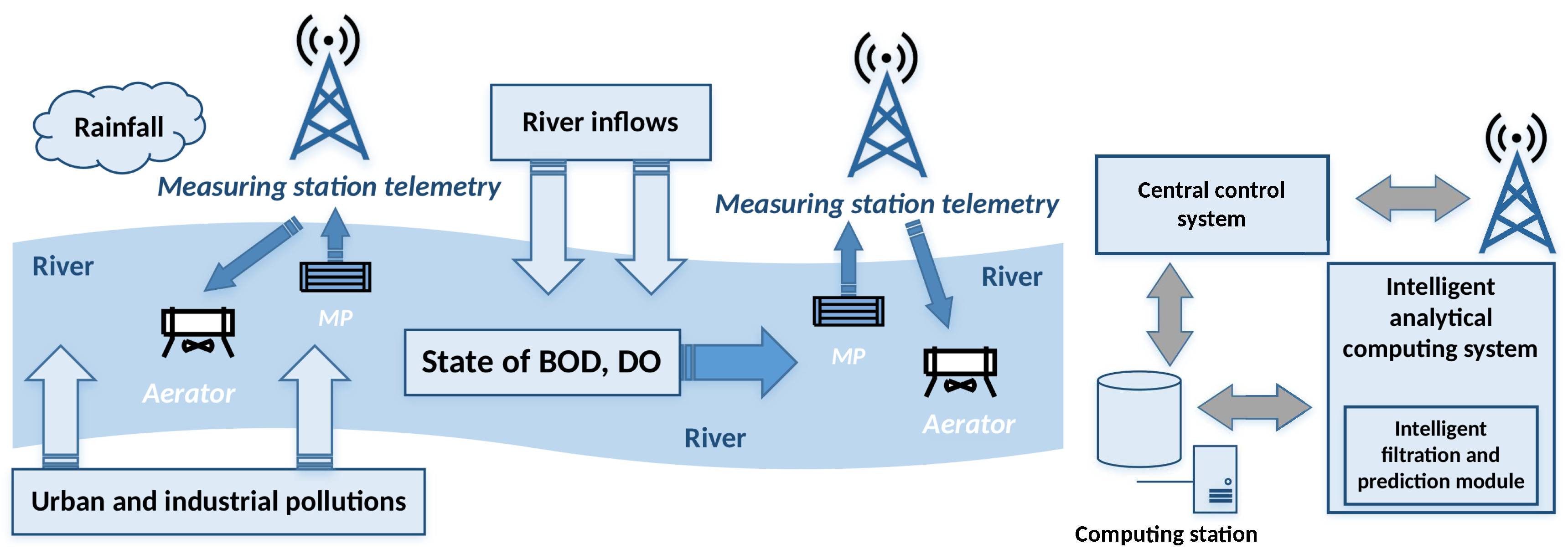
Contaminated water, partially or completely polluted as a result of household, industrial, agricultural and other uses is commonly referred to as waste water. The largest part of the pollution in waste water contains detergents, organic matters and oils. There are different approaches for removing these contaminants or eliminating them. We can divide them into two groups of methods: artificial or natural. The first method uses a set of filters: mechanic filters (for precipitation, flocculation, trapping pollutants by organisms and by hyporheic sediment, sorption on mineral and organic particles), chemical filters (for chemical degradation of pollutant, as abiotic oxidation and photo-oxidation) and biochemical filters (biodegradation of pollutants, assimilation). The second method, also referred to as self-purification, is a natural process of rivers, lakes or canals to recover the rate of dissolved oxygen values of the highest concentration of oxygen, which is one of the best indicators of water quality. The self-purification process of water bodies are processes involving biological, chemical and physical processes working simultaneously on biological pollutants, oxidizing them and increasing the amount of dissolved oxygen. Self-purification of running waters is a set of natural processes that are present in rivers and streams, enhanced by water turbulence that helps to increase the amount of oxygen to dissolve in the water. The self-purification aspect and its control provide the leading motive of this paper [1,2,3,4]. A problem of paramount importance to contemporary societies is determining how to best retain the quality of stream water and maintain acceptable levels of dissolved oxygen concentrations using a variety of pollution control activities. For the prediction of dissolved oxygen in a stream under scenarios of interest, different heuristic and deterministic models have been applied in the past [5,6]. Neural networks are a proven and effective tool for diagnosing and controlling difficult-to-measure processes where precise parametrization of a mathematical model is difficult or even impossible [7,8]. In recent years, ANN have found a number of applications in the area of water quality modeling. A good review of the applications of ANNs in water quality modeling was summarized by the American Society of Civil Engineering (ASCE) task committee on the application of Artificial Neural Networks in hydrology, ASCE [9]. Recently, several methods involving intelligent soft computing techniques have been proposed [10,11]. Taormina et al. proposed in [12] data-driven base-flow separation-based modular models for the prediction of stream-flow discharge. Wu et al. proposed in [13] the use of a modular artificial neural network for improving rainfall prediction. In addition, the advantages of techniques with particle swarm optimizations for downstream river flow forecasting have been proposed in [14]. Daily rainfall prediction has been modeled with a hybrid model integrating artificial neural networks and support vector regression [15]. Based on the authors’ collective knowledge and previous experience in mathematical modeling of a river object [8,16,17,18,19,20,21] and preliminary concepts presented in [22], we propose in the paper a novel intelligent system that monitors and controls the quality of water in a river using ANN (Figure 1). The conceptual diagram represents a river fragment and its banks, along which are placed telemetry stations, sampling points Measurement Point (MP) and devices for aeration of monitored river sections.

The main river current is fed with lateral inflows, atmospheric precipitation and urban and industrial inflows, which are the most frequent sources of biochemical pollution of the river. When the river becomes contaminated, the only way to reduce the negative impact is to provide oxygen directly to the water, consequently protecting the biological life of the river. The intelligent analytical computing system module continuously monitors two basic BOD and DO water quality indicators. These indicators are crucial for assessing the ecological status of the river water and possible related hazards to living organisms. The results for the DO measurement are immediate, while the measurement of the BOD parameter is difficult to achieve in real time as it is performed in a laboratory environment over a period of 5 to 28 days. The proposed monitoring system utilized mathematical models of the river and performs the estimation of difficult-to-measure variables. In this circumvention, we will utilize the measurement of dissolved oxygen to determine the value of biochemical oxygen demand [23,24,25,26]. In the experimental part of the actual work, the object to which the proposed system is applied is the Wislok river, located in the southeastern part of Poland. Its hydrological profile and actual measurement data have been used to determine the value of control and monitoring parameters implemented by the intelligent analytical computing system.

2. Methods

2.1. Mathematical Model of Water Quality

Mathematical biochemical models of levels of water pollution in rivers had various forms depending on their application in order to present their components and dependencies. They are used for the equation of quantitative description. These are (usually differential) equations that link important values like input, output and variable states. Oxygen balance is the basis for water contamination modeling; it is described by two indicators of water quality: BOD and DO. Biochemical oxygen demand equals the amount of oxygen used by aerobic microorganisms over a specific time period and conditions, for oxidation of organic compounds in water or waste-water [27]. This value determines the content of biodegradable organic compounds. Dissolved oxygen is an indicator that has a significant influence on chemical and biochemical processes in water. The indicator is also crucial for organisms that create river ecosystems. Studies conducted by Streeter and Phelps in relation to BOD and DO concentration in rivers are the basis for mathematical modeling of water quality [3]. The equations describe the biochemical decomposition of organic compounds, which runs according to the first order differential equation of physical-chemical reaction kinetics. Dependency for a steady volume of water and contamination takes the form of [19,22,28,29,30,31,32]:

$$\frac{d{x}_1}{dt}=-k_1{x}_1+w_1,x_1\left(t_0\right)=x_{10},$$

(1)

where $x_1^{}$ = (mg/L)—BOD concentration, t (day)—time, $k_1$ (1/day)—reaction rate coefficient, and $w_1$ (mg/(L·day))—intensity of BOD pollution loads. The change of oxygen dissolved in water:

$$\frac{d{x}_2}{dt}=-k_2{x}_1+k_2\left(x_{2N}-x_2\right)+a,x_{2N}\left(t_0\right)=x_{20N},$$

(2)

where $x_2$ = (mg/L)—DO concentration, t (time)—time, $k_2$ (1/day)—rate coefficient of BOD influence DO, $k_3$ (1/day)—rate coefficient of oxygen absorption from air, $x_{2N}$ (mg/L)—oxygen content in water saturation, a (mg/L·day)—intensity of oxygen absorption or consumption. In further considerations, to present DO processes in a simpler way, DO deficit is used. Therefore, assuming that $x_2$ is DO deficit interpreted as:

$$x_2=x_{2N}-x_{2s},$$

(3)

where $x_{2s}$ represents value $x_2$ from Equation (2). We get a dependency that describes the change of DO deficit in time:

$$\frac{d{x}_2}{dt}=-k_2{x}_1+k_3{x}_2+a,x_2\left(t_0\right)=x_{20}.$$

(4)

Equations (1) and (4) can be written in the form of vector:

$$\frac{dx}{dt}=Ax+Bw,$$

(5)

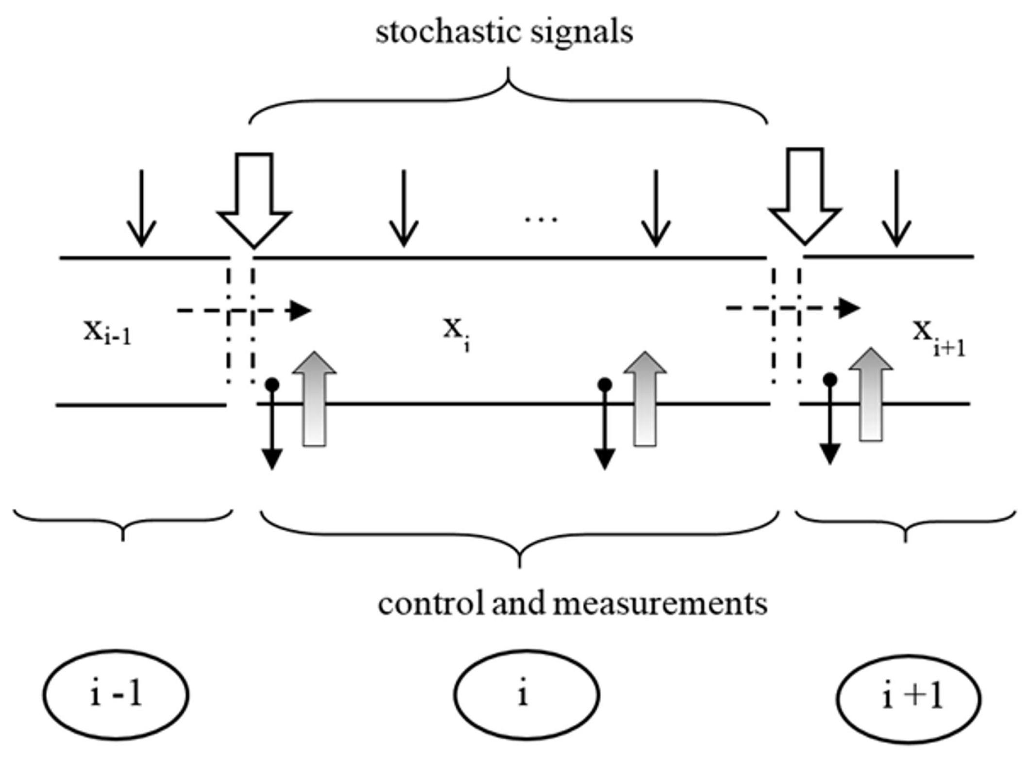
where $A=\left[\begin{array}{cc}-k_1& 0\\ -k_2& -k_3\end{array}\right]$ state matrix, $x=col\left[\begin{array}{cc}{x}_1& x_2\end{array}\right]$—state vector (BOD and DO, respectively), B—control matrix, and w—vector of external extortion and alternatively of controls. A river can be divided into smaller parts, interpreted separately. Taking into consideration longer segments of the river, the outflow from one tank is the inflow of another (Figure 2).

Due to the nature of the phenomena in rivers [4], there is one direction of the transport of state vector, the changes of which are imposed by the processes (self-purification, diffusion). Considering the river divided accordingly into cascade segments where the time of river flow depends on the rate of river flow. The current studies concern observations of a water section moving freely, affected by side inflows. The length of river that results from the rate of flow can be adequately used instead of the time axis.

2.1.1. Models with Distributed Parameters

Conducting an analysis of the state vector $x\left(z,t\right)$ dependent on the time and length of the river, Streeter–Phelps Equations (1) and (4) including mass balance are transformed into the first order hyperbolic partial differential equations. BOD–DO mathematical model for i-th river segment is described with the equation [22,33]:

$$\frac{\partial }{\partial t}{x}_i+\frac{\partial }{\partial t}{V}_i{x}_i=A{x}_i+B{w}_{ri},$$

(6)

with boundary conditions $x_i\left(0,t\right)$, $x_i\left(z,t_0\right)$ where: $x_i$—state vector of ith segment, t—time, z—length, A—matrix of interactions, $w_{ri}$—distributed disturbance vector, and $V_i=\left[\begin{array}{cc}{v}_i& 0\\ 0& v_i\end{array}\right]$—diagonal matrix of river flow speed. The model considers the boundary conditions represented by: edge condition, which describes the starting point of the considered segment in the time domain:

$$x_i\left(0,t\right)=M_i{x}_{i-1}\left(1,t\right)+w_{bi}\left(t\right)+R_{bi}{u}_{bi}\left(t\right).$$

(7)

Matrix $M_i$ represents the edge interrelations between single segments, vector $w_{bi}$ refers to the edge disturbances. Control $u_{bi}$ has an impact only on a state vector coordinate $x_2$ and on locating it at the starting point of the river segment. Initial disturbance concerns the whole segment at a moment $t=t_0:$

$$x_i\left(z,t_0\right)=x_{i0}\left(z\right),i=1,2,\dots ,N.$$

(8)

The mathematical model described by the first order hyperbolic partial differential Equation (6) represents a general approach. Using a different interpretation of this model, an equivalent description can be used with the set of Streeter–Phelps equations (description in Section 2.2) [19,20,21,22].

2.1.2. Second Order Distributed Parameter Model

In water environments there are multiple factors that influence the water quality. The aim is to attempt to consider all the conditions that have an impact on the self-purification process. The diffusion is a factor that influences the water condition and is considered regarding spatial conditions such as: length, width and depth. Using the Gauss–Ostrogradsky theorem, the model of diffusion can be written in the form of a second order partial differential equation. The general form of the diffusion equation is:

$$\frac{\partial x}{\partial t}-div\left(Dgradx\right)+\delta =0,$$

(9)

in which x—state vector dependent on the time and spatial parameters, D—isotropic diffusion coefficient, and $\delta$—intensity of production or loss of shifted factor. Based on Equation (9), the river state vector is considered dependent on time, length, width and depth taking into consideration the river self-purification process, the diffusion equation is:

$$\frac{\partial x}{\partial t}-\left(D\frac{{\partial }^{2}x}{\partial z_1^2}+D\frac{{\partial }^{2}x}{\partial z_2^2}+D\frac{{\partial }^{2}x}{\partial z_3^2}\right)+Ax+\delta =0,$$

(10)

where $z_1,z_2,z_3$ describe the coordinates of length, width, depth, A—state matrix. Assuming that the change of diffusion along the variable spatial depth of water is negligibly small against the width and length of body of water in the Equation (10), the last component can be excluded. Completing the Equation (10) with the flow speed, an additional component appears:

$$\frac{\partial x}{\partial t}-\left(D\frac{{\partial }^{2}x}{\partial z_1^2}+D\frac{{\partial }^{2}x}{\partial z_2^2}\right)+V\frac{\partial x}{\partial z_1}+Ax+\delta =0,$$

(11)

where V is a diagonal matrix that represents the flow speed in a given segment length. Solving the above equations is possible in variable boundary conditions:

$$x\left(z_1,t_0\right)=f_{p1}\left(z_1\right),$$

(12)

$$x\left(z_2,t_0\right)=f_{p2}\left(z_2\right),$$

(13)

$$x\left(0,t\right)=f_b\left(t\right),$$

(14)

where functions $f_{p1},f_{p2},f_b$ are known for particular coordinates.

2.2. Ordinary Differential Equations on Characteristics

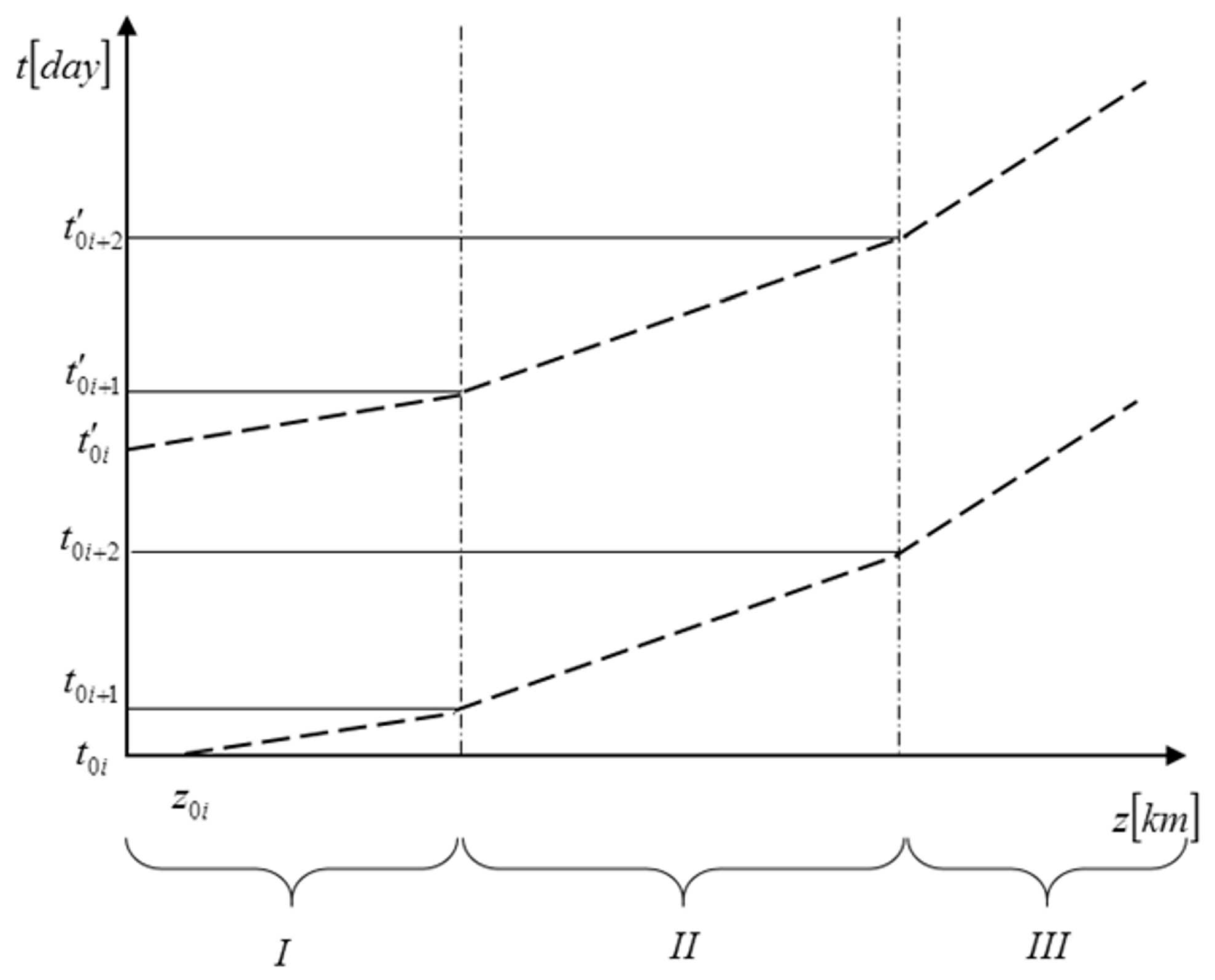
The function that describes the values of state coordinate x in the space-time field is the solution of hyperbolic partial differential equations. It means that values of this function are available for any length of river and any period of time in this field. Using the idea of this solution and considering a natural flow, a modified interpretation of the mathematical model of the river water pollution described by the Equation (6), which, without losing the model accuracy, utilize the river self-purification process was proposed. Positive values of the diagonal V matrix in Equation (6) causes Streeter–Phelps equations to have common characteristics along which they become ordinary equations. The question comes down to the analysis of river self-purification process along the characteristics (Figure 3) of space-time field concerning the speed of BOD and DO pollution relocation.

The levels of water pollution in the river considered along the characteristics in the field $z\in \left[0,1\right]$ and $t\in \left[t_0,t_k\right]$, $t_k<\infty$ become ordinary differential equations that represent respective characteristics. The description of particular segments leads to the solution of a particular number of space-time field characteristics. The characteristics of ith river segment are defined with dependency:

$$\frac{d}{dt}{z}_i\left(t\right)=v_i\left(z_i\left(t\right)\right),$$

(15)

the edge points of which meet the condition:

$${\int }_{t_{0,i}}^{t_{0,i+1}}{v}_i\left(z_i\left(t\right)\right)dt+z_{0i}=1,$$

(16)

in which $z_{0i}\in \left[0,1\right]$ is the initial coordinate in the moment $t_{0i}$. For the same characteristic, the moment $t_{0i+1}$, determines the starting point in i+1-st segment. A set of line segments of the characteristic covers the space-time field, to which further considerations regarding the issues of river state estimation [20,32,33,34,35] will be related. Measurements continuous in time can be performed at specified control points along the river. The considerations concern a boat drifting freely with the river current. Shifting down a particular river, encountering the located control points, the measurements taken for a given characteristic become discrete in time. Continuous measurements are described with the equation [33,34]:

$$y\left(t\right)=x_2\left(t\right)+v_p\left(t\right),$$

(17)

where $x_2$—dissolved oxygen, and $v_p$—measurement disturbance with Gaussian distribution. Substituting $t=t_k$, for k = 1, 2, 3, …, we obtain a measurement discrete equation:

$$y\left(t_k\right)=Cx\left(t_k\right)+v_p\left(t_k\right),$$

(18)

in which the state vector $x\left(t_k\right)=col\left[\begin{array}{cc}{x}_1\left(t_k\right)& x_2\left(t_k\right)\end{array}\right]$, matrix $C=\left[\begin{array}{cc}0& 1\end{array}\right]$ and measurement disturbances are determined in discrete measurement moments $t_k$.

The equation for i-th river segment can be written in the form of ordinary differential equations on characteristics:

$$\frac{d}{dt}x\left(z_i\left(t\right),t\right)=A\left(z_i\left(t\right)\right)x\left(z_i\left(t\right),t\right)+B{w}_r\left(z_i\left(t\right),t\right),$$

(19)

with initial condition: $x\left(z_i\left(t_0\right),t_0\right)=x_0\left(z_{i0}\right)$ for $i=1,2,3,\cdots$. The edge conditions disappear because the characteristic concerns the whole field of considerations for the river [33,34].

2.3. River State Estimation with Kalman–Bucy Filter

The problem of state estimation $x\left(t\right)$ comes down to the determination of the estimate $\widehat{x}\left(t\right)$ of the current state, considering the condition for the minimization of distance between $x\left(t\right)$ and its estimate $\widehat{x}\left(t\right)$. It is reduced to the solution of differential equation [32,33,34]: $\frac{d}{dt}\widehat{x}\left(t\right)=A\widehat{x}\left(t\right)+K\left[y\left(t\right)-C\widehat{x}\left(t\right)\right]$, where $\widehat{x}\left(t_0\right)=\widehat{x}\left(t\right)$ in which the enhancement filter coordinate $K_F$ is determined with the equation:

$$K_F\left(t\right)=P\left(t\right)C^T{V}_p^{-1},$$

(20)

where V is the measurement error covariance, and estimate error covariance matrix P(t) is obtained with a Riccati differential equation:

$$\frac{\partial P\left(t\right)}{\partial t}=AP\left(t\right)+P\left(t\right)A^T-P\left(t\right)C^T{V}_p^{-1}CP\left(t\right)+D{W}_r{D}^T,$$

(21)

with starting condition $P\left(t_0\right)=P_0$. Matrix $W_r$ is the covariance matrix of system disturbances $w_r$ that are present in the Equation (19). Therefore, in order to obtain state estimate $\widehat{x}\left(t\right)$ first, it is necessary to solve the Riccati Equation (21), next based on its solution to determine the enhancement filter coordinate $K_F\left(t\right)$ (20) and finally solve the estimates Equation (19). When considering the issue of estimate, “along the characteristics”, it is necessary to pay attention to the measurement equations that become discrete in time. This results in the characteristic $z_i\left(t\right)$ encountering control points in $z_{i1},z_{i2},\dots$, which correspond with discrete time moments $t_{1i},t_{2i},\dots ,t_{mi}$. As a result, the equation takes the form:

$$y_i\left(t_{mi}^i\right)=C_i{x}_i\left(z_i\left(t_{mi}^i\right),t_{mi}^i\right)+v_{pi}\left(t_{mi}^i\right),$$

(22)

in which $v_{pi}\left(t_{mi}\right)$ is Gaussian white noise with zero mean and covariance:

$$E\left\{v_{pi}\left(t_k\right)v_{pi}{\left(t_k\right)}^T\right\}=V_p\left(tk\right){\delta }_{kl},$$

(23)

where $t_k$—measurement moment, E means the expected value operator, and ${\delta }_{kl}$—Kronecker function which:

$${\delta }_{kl}=\left\{\begin{array}{cc}0,& for\\ 1,& for\end{array}\begin{array}{c}\\ \end{array}\right.\begin{array}{c}k\ne l,\\ k=l.\end{array}$$

(24)

The proposed approach allows the mathematical model of river with centered parameters to be described, but the questions that occur here are for the objects with distributed parameters that are represented by time moments $t_{1i},\dots ,t_{mi}$. In the estimation process that comprises continuous and discrete measurements, two stages can be distinguished: filtration and prediction. The prediction and filtration equations are obtained based on a Kalman–Bucy filter [33,36] in which measurement continuity is included, assuming that: $V_p\left(t\ne t_k\right)=\infty$. In the filtration stage estimates are obtained in moment $t_k$ based on the estimates from previous time moment $t_{k-1}$ and current measurements. This process is described with the following equations:

$$\widehat{x}\left(t_k/\phantom{t_k{t}_k}{t}_k\right)=\widehat{x}\left(t_k/\phantom{t_k{t}_{k-1}}{t}_{k-1}\right)+K_F\left(t_k\right)\left[y\left(t_k\right)-C\widehat{x}\left(t_k/\phantom{t_k{t}_{k-1}}{t}_{k-1}\right)\right],$$

(25)

$$\widehat{x}\left(t_0/\phantom{t_0{t}_{-1}}{t}_{-1}\right)={\overline{x}}_0,$$

(26)

$$P\left(t_k/\phantom{t_k{t}_k}{t}_k\right)=P\left(t_k/\phantom{t_k{t}_{k-1}}{t}_{k-1}\right)-K_F\left(t_k\right)CP\left(t_k/\phantom{t_k{t}_{k-1}}{t}_{k-1}\right),$$

(27)

$$P\left(t_0/\phantom{t_0{t}_{-1}}{t}_{-1}\right)=P_0,$$

(28)

$$K_F=P\left(t_k/\phantom{t_k{t}_{k-1}}{t}_{k-1}\right)-C^T{\left[CP\left(t_k/\phantom{t_k{t}_{k-1}}{t}_{k-1}\right)C^T+V_p\left(t_k\right)\right]}^{-1},$$

(29)

where $\widehat{x}\left(t_k/\phantom{t_k{t}_k}{t}_k\right)$—estimate in moment $t_k$ obtained based on the measurements $y\left(t_0\right),\dots ,y\left(t_k\right)$, $P\left(t_k/\phantom{t_k{t}_k}{t}_k\right)$—estimate covariance error, and $K_F\left(t_k\right)$—enhancement filter coordinate. The prediction is based on finding an estimate prior to the next measurement moment for $t\in \left(t_k,t_{k+1}\right)$, taking the estimates obtained in the filtration process for the initial values. The prediction is presented with the equations:

$$\frac{d}{dt}\widehat{x}\left(t/\phantom{t{t}_k}{t}_k\right)=A\left(t_k\right)\widehat{x}\left(t/\phantom{t{t}_k}{t}_k\right),$$

(30)

$$\widehat{x}\left(t_k/\phantom{t_k{t}_k}{t}_k\right),$$

(31)

$$\frac{d}{dt}P\left(t/\phantom{t{t}_k}{t}_k\right)A{\left(t_k\right)}^T+A\left(t_k\right)P\left(t/\phantom{t{t}_k}{t}_k\right)+W_r,$$

(32)

$$P\left(t/\phantom{t{t}_k}{t}_k\right),$$

(33)

where $\widehat{x}\left(t_k/\phantom{t_k{t}_k}{t}_k\right)$, $P\left(t_k/\phantom{t_k{t}_k}{t}_k\right)$—estimate and covariance of estimation error estimated for $t>t_k$, and W${}_r$—disturbance covariance w${}_r$ [22,32,34]. The results relevantly depend on the accurate determining of Stochastic Processes that include force signals. Practical experience shows that the influence of weather conditions decides on the characteristics of the signals mentioned above. Thus, it is advised to update these characteristics frequently for a more precise determination.

2.4. Model of Feed-Forward Neural Network

Artificial neural networks are already well established as a proven data analysis tool. In this section, we briefly review supervised feed-forward neural network with the back-propagation learning strategy. Figure 4 presents the exemplary two-layer ANN regarding typical Matlab (R2013a (8.1.0.604), MathWorks, Natick, MA 01760-2098, United States) environment notation of the input pattern P and output activations A ,respectively.

Input signal to the j-th neuron in the first layer:

$$e_1\left(j\right)=\sum _{i=0}^I{w}_1(i,j)P\left(i\right),$$

(34)

where $w_1(i,j)$—an element of $W_1$ matrix connecting receptor layer with first layer of neurons, i—receptor number, j—neuron number in the input layer, and $P\left(i\right)$—denotes i-th element of input vector. For the sake of simplicity, shifting elements $b_l$ are included in the weights matrix. Neurons activation in the first layer is expressed as $a_1\left(j\right)=h\left(e_1\left(j\right)\right)$, where $h\left(e_1\left(j\right)\right)$ denotes the neuron transfer function in the first layer. Similarly, the input signal to the k-th neuron in the second layer equals $e_2\left(k\right)={\sum }_{j=0}^J{w}_2(j,k)a_1\left(j\right)$, where $w_2(j,k)$ is an element of weight matrix $W_2$ connecting the first and second layer. Per analogy, the activation of neurons in second- output layer is expressed as:

$$a_2\left(k\right)=h\left(e_2\left(k\right)\right)=h\left(\sum _{j=0}^J{w}_2(j,k)h\left(\sum _{i=0}^I{w}_1(i,j)P\left(i\right)\right)\right).$$

(35)

Usually, the sigmoid function is assumed to be the transfer function of a particular neuron because of the simple numerical computation complexity of its first derivative:

$$h\left(e\right)=\frac{1}{1+exp(-e)}\frac{\partial h\left(e\right)}{\partial e}=h\left(e\right)\left(1-h\left(e\right)\right).$$

(36)

Other differentiable transfer functions like linear, logarithmic, hyperbolic tangent or Gaussian can also be used. The set of weights $w_1(i,j)$ and $w_2(j,k)$, usually randomly generated at the beginning of training process, does not provide required network knowledge functionality. The correction of weights in the consecutive steps of training, known also as epochs, stands the classic task for the network trained with supervisor. Such ANN architecture has the error function, also referred to as cost function defined as follows:

$$E=\frac{1}{2}\sum _q{\left[T^q\left(k\right)-h\left(\sum _{j=0}^J{w}_2^q(j,k)h\left(\sum _{i=0}^I{w}_1^q(i,j)P^q\left(i\right)\right)\right)\right]}^2,$$

(37)

where q—denotes the number of the consecutive input vectors with appropriate target output vector $T^q$. This equation is referred to as least-square-method and its internal part might be modified according to the class of the considered problem to be solved. The only two requirements that have to be satisfied in general cases: internal expressions are differentiable and its common minimum exists, such that: $E\to 0$ [37]. In recent works [17,18], we have observed that, in general cases, the order of derivatives does not have to be of integer values and this advantage provides fluent modification of neuron transfer function dynamics and its control during the ANN training process. The expected changes of weights under the training procedure are expressed with the equation:

$$w^{(q+1)}-w^{\left(q\right)}=\mathsf{\Delta }{w}^{\left(q\right)}=-\eta \frac{\partial E^{\left(q\right)}}{\partial w},$$

(38)

where $\eta$—denotes the learning rate coefficient, usually in the range 0.1–1.5. At the experimental part, we used the set of scripts from Matlab Neural Network Toolbox (Matlab NNET) library as well as our own scripts with fluent modification neuron features functionality. The modified version of backpropagation algorithm regarding momentum mechanism and reinforcement learning rule also referred to as Quick Propagation (QuickProp) has been utilized as weight changing rule:

$$\mathsf{\Delta }{w}_{NEW}(i,j)=m_c\mathsf{\Delta }{w}_{OLD}(i,j)+(1-m_c)\eta P\left(i\right)\delta \left(j\right),$$

(39)

where $\mathsf{\Delta }{w}_{NEW}$ and $\mathsf{\Delta }{w}_{OLD}$ denotes weights corrections in consecutive steps. In this circumvention, momentum coefficient value equals $m_c=0.1$ and does not change during training process, opposite to learning rate coefficient which changes with strategy: $\eta =1.05\times \eta$—if new computed error decrease its value along training time, $\eta =0.7\times \eta$—otherwise. With this circumvention, the training process can be accelerated, preserving at the same time the ability of ANN to overcome the local minimum traps in the error function space.

2.5. Artificial Neural Networks for Estimation Processes

By using information about the current state of the river and anticipated changes in river pollution the monitoring and control system has been designed (Figure 5).

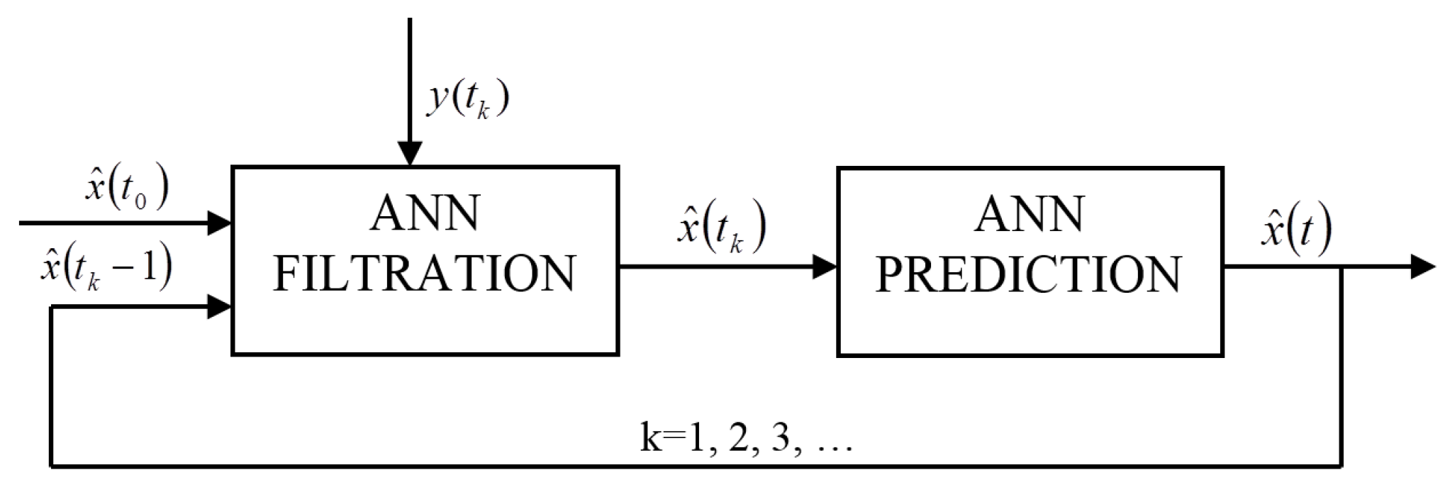
The purpose of the system is to monitor the quality of water, and, in the event of threats to its lifeforms, respond accordingly by reducing the effects of emerging pollutants. Its primary function is to predict the state of water quality in real time because of the ravages occurring when delayed response to impurities leads to irreversible ecological changes in the river. The monitoring system based on DO measurements and BOD estimation performed by neural networks is able to determine the current values of river pollution indicators. The system also predicts their changes over an assumed time interval. Using this information system generates appropriate controls for water aeration devices in the river. This is a key mechanism to safeguard the life forms of the river and the water quality. Using the Kalman–Bucy filter in the state estimation process requires knowledge of the characteristic features of extortion processes such as disturbances effecting the system and measurements. It usually involves great amounts of work and does not always lead to satisfactory results. Using artificial neural networks is an alternative solution, which will support the execution of filtration process thanks to its properties [8,17,38,39,40,41]. The studies employed feed-forward artificial neural networks and training based on backpropagation algorithm. Taking into consideration the complexity of questions that result from the measurement comparison of discrete and continuous objects, it is difficult to find one structure of neural network that would generate estimates with satisfactory results. This is the reason why two separate structures of artificial neural networks were used, as in the case of the filtration and prediction process Figure 6. Obviously, these networks cooperate with one another according to the algorithm of estimation that uses the filtration and prediction processes [4,21,22,32,34].

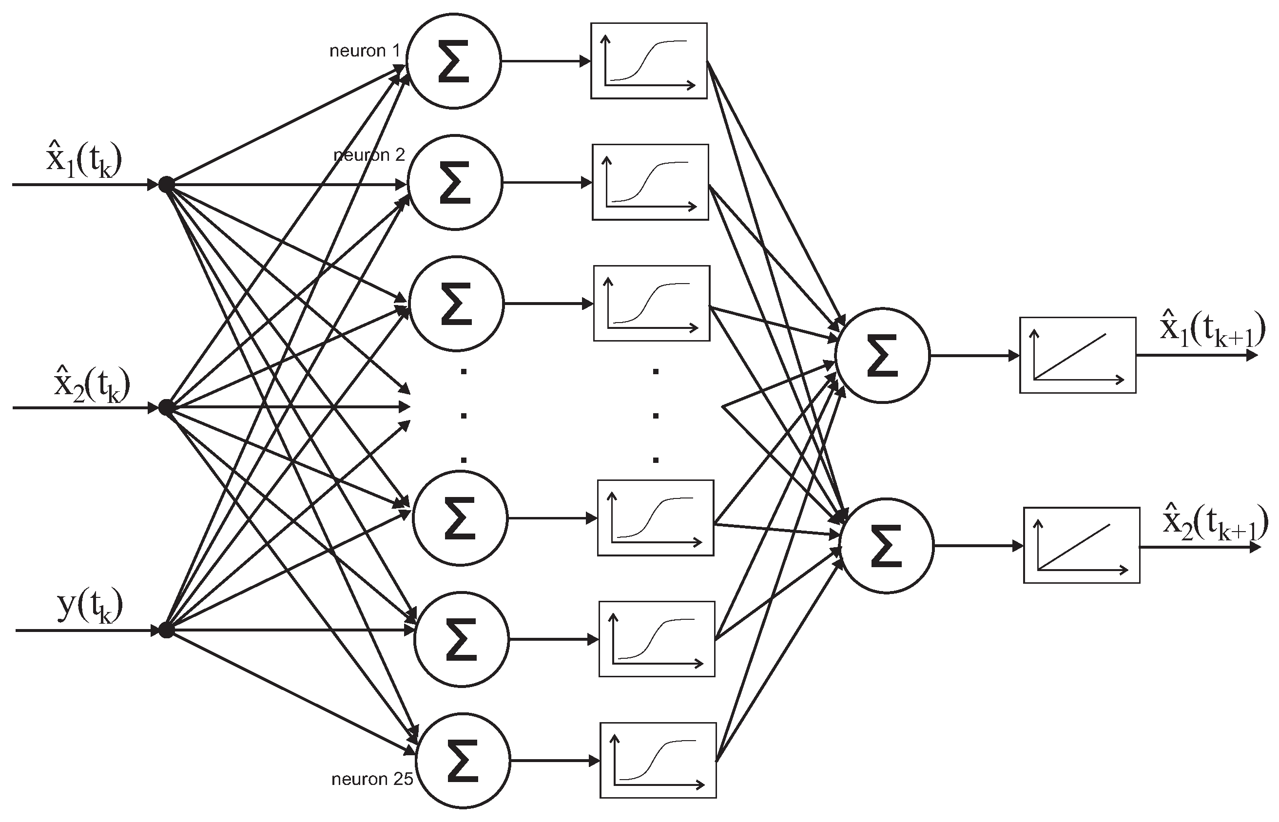
The value of estimates from the previous moment and the value of measurement were given at the system input. In the ANN training process, we trained both network modules with the target values of estimates obtained from the mathematical model. The execution of filtration process is the first stage. The output signal of this part of the system are the estimates values in discrete measurement moments which are the input signals for the second ANN structure in the prediction process. As a result, the estimate values of BOD and DO are obtained, which are given with the feedback loop at the system input. The structure of neural network for the filtration (see Figure 7) stems from the logic of functioning of this process. The BOD and DO state estimate is obtained at the output in discrete measurement moments. The input signals are the state estimates determined before the measurement moments and the measurement signal. Thus, in the input layer, there are three receptors (two state vector coordinates and measurement), and the output layer comprises two neurons that generate estimates in measurement moments.

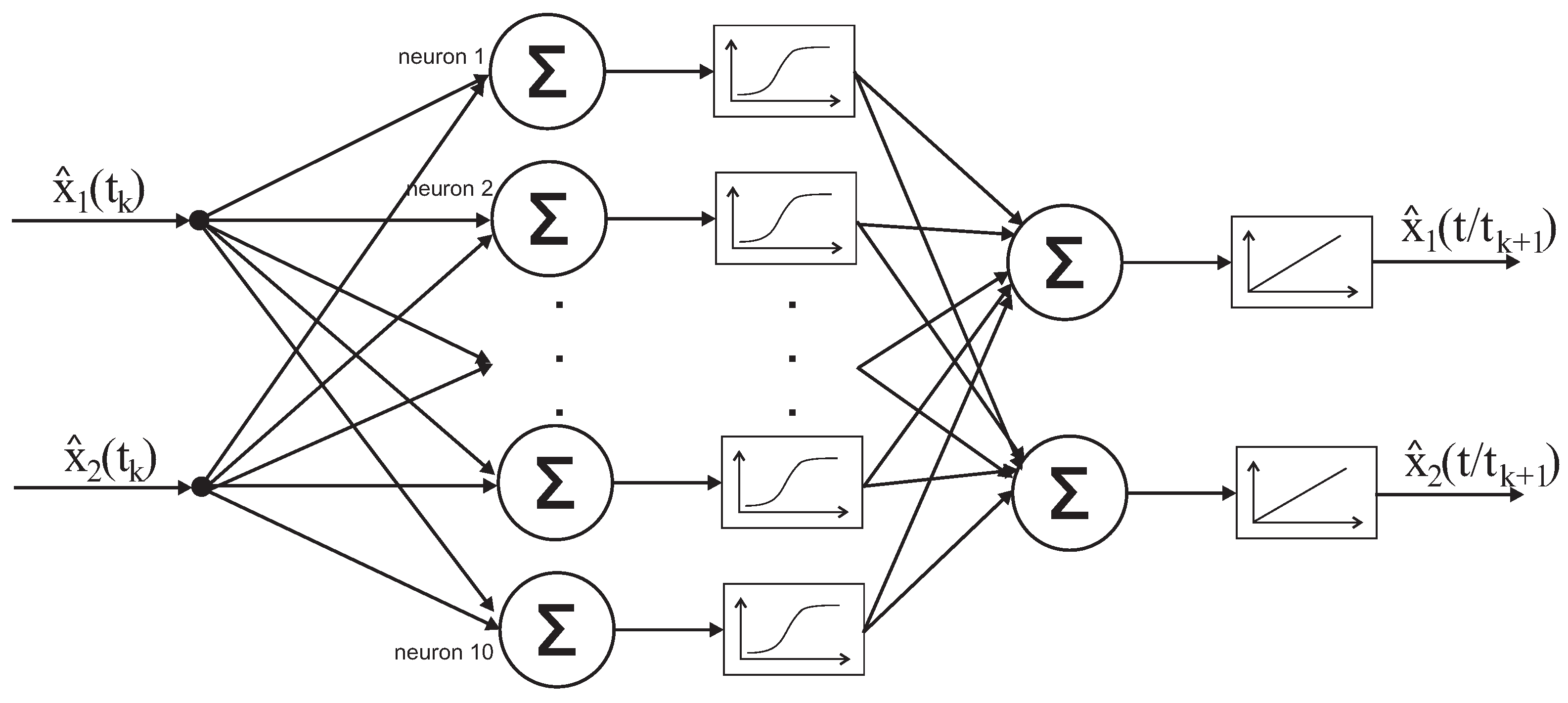
The amount of neurons in the hidden layer and the selection of activation function are the result of experimental studies. The activation function in the hidden layer is sigmoid, and linear in the output layer, in order not to restrict the values of output signals obtained from the network. It is worth mentioning that such network architecture represents one characteristic for one execution of the filtration process. In order to obtain state estimates for multiple characteristics, it is necessary at the network input to give the current measurement and corresponding estimates values connected with a particular characteristic. The prediction process runs interchangeably with the filtration process and executes a task, which is to obtain BOD and DO estimate values obtained in the filtration process. In the river control system [42], this process must closely cooperate with the filtration and deliver information concerning the river condition between conducted measurements. The network architecture is similar to the filtration process, while in the input and output layer, there are only two neurons, and the amount of neurons in the hidden layer can have different values. In the prediction in the hidden layer a sigmoid activation function was used, and linear one was used in the output layer [22,32,34]. During the training of networks, different BOD and DO state values can be used. The neural network diagram in the prediction process is presented in Figure 8.

The quality of estimates obtained in the filtration or prediction processes depends on the process of network training during which the network changes the amount of neurons in the hidden layer. The network training process has a significant influence on the results. When a great variety of cases of model signals are taken into consideration, the generated estimates will correspond to the expectations. The length of the training process affects the estimates obtained from the neural networks. When the network training error is too large, it means that the network was not sufficiently trained, but it is able to generate the estimates burdened with very large errors. In extreme cases the neural network can distort the estimate process against its real state. It concerns large and sudden state changes that can be caused by side inflows of high pollution level. Using the proposed approach, one can obtain the river state estimate with the use of artificial neural networks. Appropriately designed ANN architecture and properly conducted training processes will allow for obtaining a system that will accurately, based on information from control points, estimate the BOD and DO change courses for a particular river segment. The artificial neural networks prepared for the filtration and prediction phase (see Figure 6) are used in the control system shown in Figure 5 in the intelligent filtration and prediction module [17,18,37,38,41,43,44,45,46,47,48]. The above approach concerns the use of two ANNs working in the system presented in Figure 6 and executing the filtration and prediction process. The creation of an artificial neural network control system which functions parallel to generating of BOD and DO estimates is a slightly different approach. ANN for BOD and DO estimate process is shown in Figure 9. At the input BOD estimate and measurements vector are given similarly like in the case of DO estimate. A two-layer neural network was used with 25 neurons in the hidden layer (Figure 7). In the case of DO, ANN in the hidden layer can have fewer neurons against BOD, e.g., 10 neurons generating correct results.

The whole set of individual learning vectors were split into two complementary sets: a training set 80% and validation set 20%. At the preliminary test stage, a subset of input vectors was randomly chosen from the set of input vectors to avoid data overfitting and maximize the ANN performance. In the main part of the experiment Matlab’s default values, i.e., for training 70%, for testing 15% and for validations 15% have been used.

2.6. The Influence of Immeasurable State Coordinates on Optimal Object Control

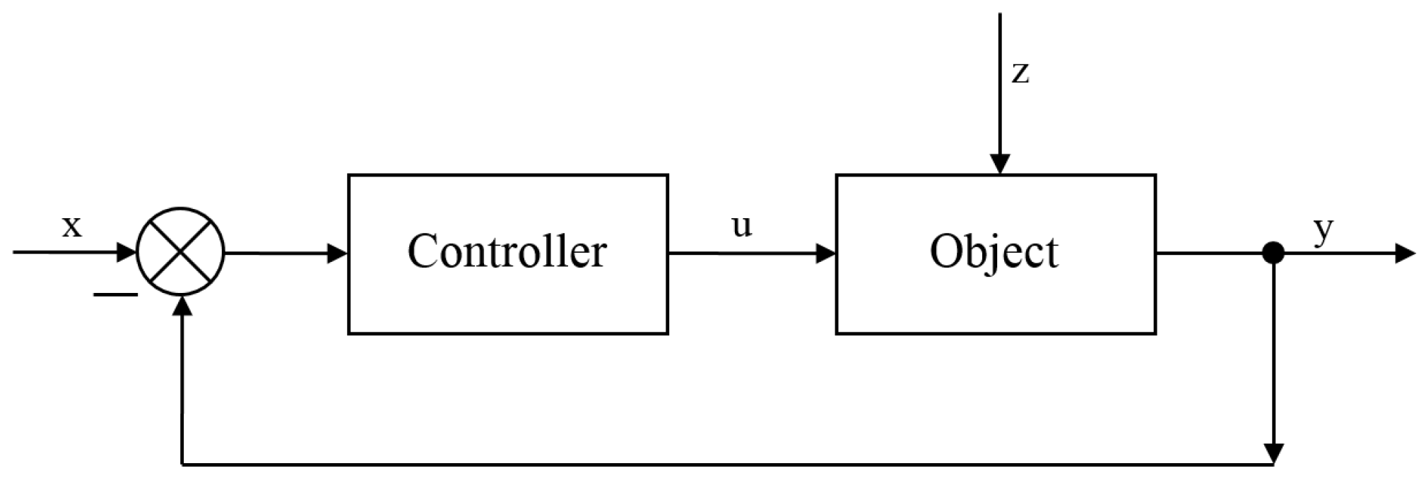
The best system according to the chosen measurement standard is called the optimal system. In order to accurately determine the optimal system, an automated regulation system comprising regulator and object is used (Figure 10), which will be described with simultaneous equations in the form:

$$\dot{x}=f\left(x,u,t\right),$$

(40)

where x—state vector of constituents x${}_1$, x${}_2$, …, x${}_n$, and u—control value vector of constituents u${}_1$, u${}_2$, …, u${}_m$, being continuous time function ranges.

In real systems, the control values are usually limited. Generally, it is assumed that the control values meet restriction in the form:

$$g_i\left(u_i,u_2,\dots ,u_m\right)\le 0fo{r}_{}i=1,2,3,\dots ,$$

(41)

where D${}_u$ is the set of acceptable control values $u\in D_u$

The quality indicator representing the optimum criteria, the goal of the function is in the form:

$$Q={\int }_0^{t_r}{f}_0\left(x,u,t\right)dt.$$

(42)

Considering a linear object described with the differential Equation (5), we assume the quality indicator as:

$$Q=\frac{1}{2}{\int }_0^{t_r}\left[x^{T}P\left(t\right)x+u^{T}R\left(t\right)u\right]dt,$$

(43)

where $P\left(t\right)$—nonnegative definite matrix of dimensions $n\times n$, and $R\left(t\right)$—positive definite matrix of dimensions $m\times m$. Additionally, we assume that regulation time $t_r$ is demanded and the control vector is not additionally restricted. The task will be to determine the control u, executing the differential Equations (5), which minimizes the quality indicators (43). The optimal control $\overline{u}$ for the presented task is determined as follows:

$$\overline{u}=\overline{u}\left(t\right)=R^{-1}\left(t\right)B^T\left(t\right)P\left(t\right)x\left(t\right)$$

(44)

where $P\left(t\right)$—symmetric matrix of dimensions $n\times n$, which constitutes the solution for the Riccati differential equation [22,32,49]. For the mathematical model of the object described with ordinary differential Equation (5), we assume the quadratic coordinate of parameters quality as follows:

$$J_Q={\int }_T\left[x^T\left(t\right)\widehat{Q}x\left(t\right)+u^T\left(t\right)Ru\left(t\right)\right]dt,$$

(45)

where $T\in \left[t_0,t_k\right]$, $t_k\to \infty$, $x\left(t\right),u\left(t\right)$—are, respectively, n and m dimensional vectors of state and control. Matrices $A,B,\widehat{Q},R$, are assumed as constants, $R>0$. River pollution levels control [25,50] is performed by introducing a particular amount of oxygen directly into the body of water. In order to select a type of control, the information specific to the current real river condition is required; then, the control will be more accurate. DO measurements can be obtained in a quick and easy way, but the obtaining of BOD value indicator is toilsome and requires laboratory conditions (BOD${}_5$ or BOD${}_{20}$), where the indicator index presents the number of days necessary to obtain credible results concerning the water polluted with organic compounds. This is why BOD values are estimated in the estimation process. For the actual considerations concerning the polluted river, we seek the controls described with the dependency:

$$u=k_{p1}\left(x_{\mathrm{BOD}}-{\widehat{x}}_{\mathrm{BOD}}\right)+k_{p2}\left(x_{\mathrm{DO}}-{\widehat{x}}_{\mathrm{DO}}\right),$$

(46)

in which: $k_{p1},k_{p2}$—are the regulator enhancement coordinates, $x_{\mathrm{BOD}},x_{\mathrm{DO}}$—BOD and DO values, ${\widehat{x}}_{BOD},{\widehat{x}}_{DO}$—state estimate for BOD and DO [22,32,42,49,51].

3. Results

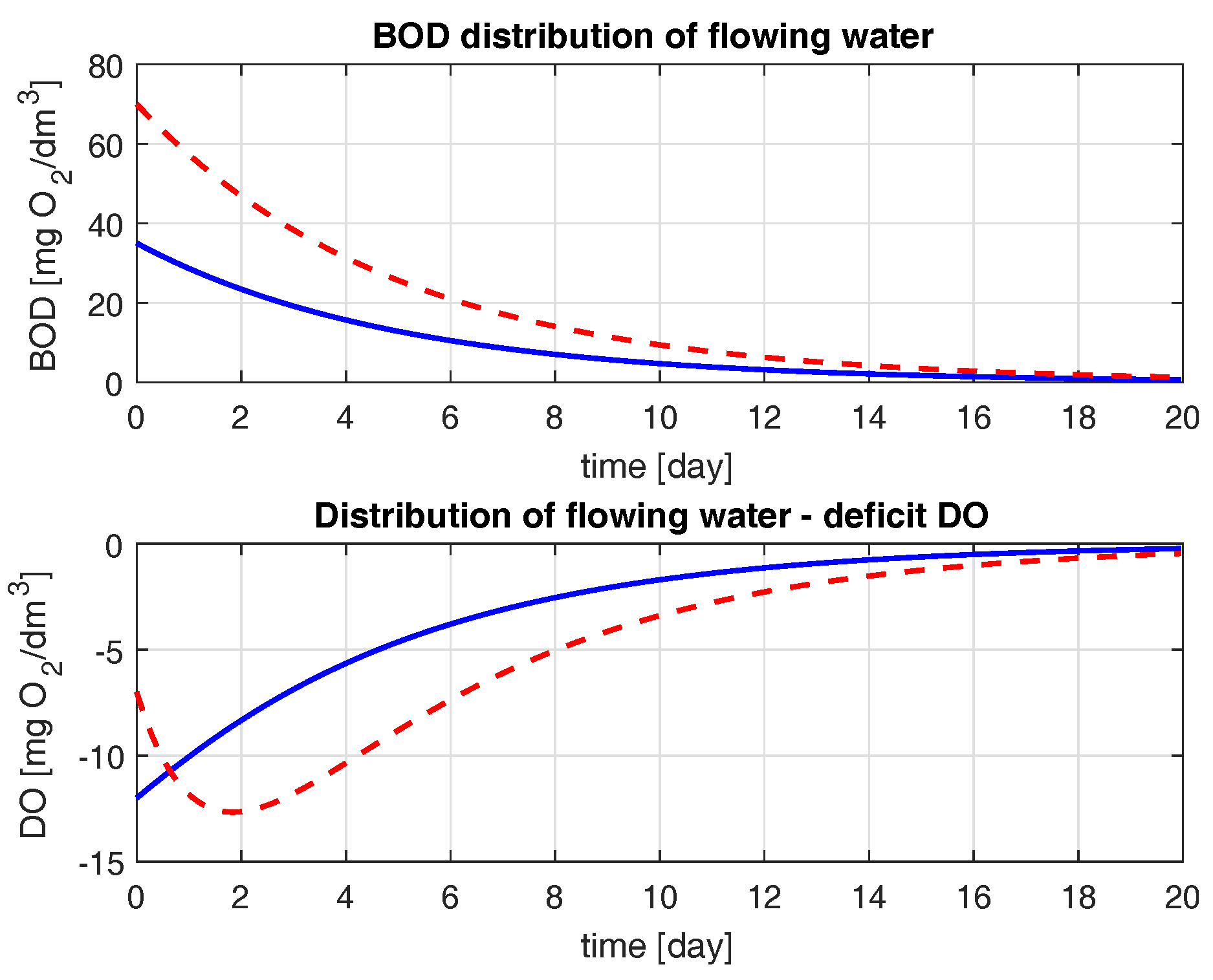
Using a river model based on the Streeter–Phelps equations, the kinetics of changes in biochemical oxygen demand and dissolved oxygen deficit has been described. The experimentations for the river described by Equations (1) and (4) has been performed according to the method described in Section 2.2. We consider the contamination state of freely flowing water, which is described by the vector $x(z,t)$. Rivers have the ability to self-clean, i.e., as pollutants increase, the values of BOD and DO decrease with the passage of time. The existence of a large deficit of dissolved oxygen at high BOD values is a natural phenomenon, which in the case of high oxygen demand generates an increase in the DO deficit. During the simulation experiments, among others, two emergency states were adopted that could occur under real conditions (see

Table 1. Initial values of parameters for the considered river section.

No.	BOD (mg/L)	DO (mg/L)	A			t (Day)	v (km/Day)
			${\mathit{k}}_1$ (Day${}^{-1}$)	${\mathit{k}}_2$ (Day${}^{-1})$	${\mathit{k}}_3$ (Day${}^{-1}$)
1	35	−12	0.2	0.185	0.71	20	20
2	70	−7	0.2	0.185	0.71	20	20

). It was assumed that a system that responds appropriately to such critical initial conditions will function properly in the real conditions of the standard levels of pollutions in the river. It was noticed that BOD had a significant influence on DO. An interesting phenomenon can be observed when inflowing pollutants have a value several times greater in mg/L. As a result, the greatest oxygen deficit (the most dangerous conditions for living organisms) can be observed after a few days and a several dozen kilometers away from the pollution inflow (see broken red line, Figure 11).

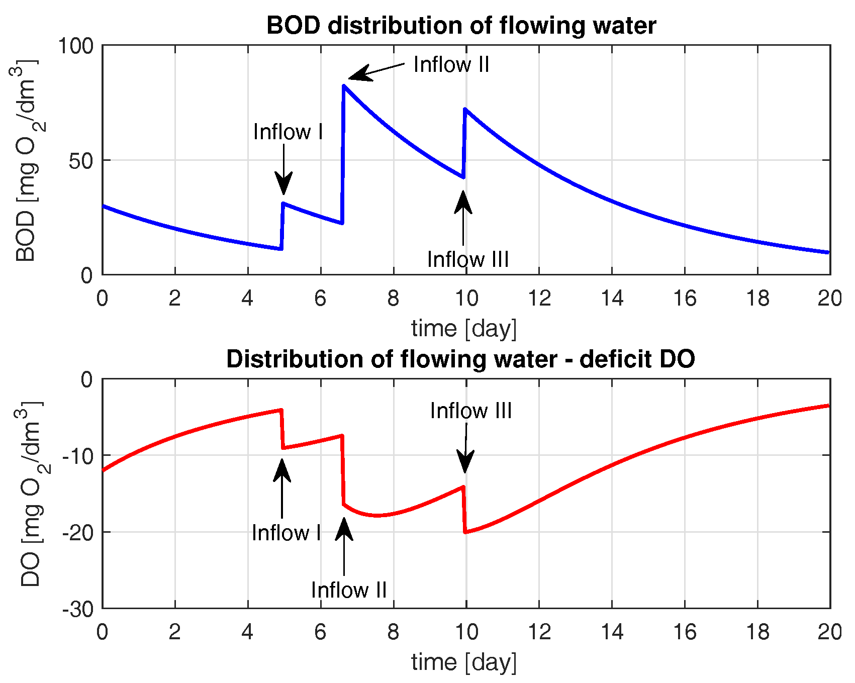
Taking into consideration a long river, it can be conventionally divided, e.g., between large inflows, and the part between them treated as a segment. The presence of large pollution inflows over a short distance causes dangerous conditions in rivers for the lifeforms. The inflows cause a significant and sudden change of BOD and DO values (see Figure 12). The observed changes in BOD and DO values with respect to lateral inflows are summarized in

Table 2. Selected parameters of the studied river section taking into account the three inflows.

Name		Value
BOD (mg/L)		30
DO (mg/L)		−12
Inflow I	BOD (mg/L)	20
	DO(mg/L)	−5
Inflow II	BOD (mg/L)	60
	DO (mg/L)	−9
Inflow III	BOD (mg/L)	30
	DO (mg/L)	−6
A	$k_1$ (day${}^{-1})$	0.2
	$k_2$ (day${}^{-1})$	0.185
	$k_3$ (day${}^{-1})$	0.71
t (day)		20
v (km/day)		20

.

The largest DO deficit was noted when the third inflow occurred after ten days of observations. The situation presented in Figure 12 shows the conditions of great oxygen deficiency for a long period of time negatively affecting the water quality that can threaten the life of organisms in the water. Analyzing the time courses, it can be observed that the largest oxygen deficit downstream “shifts” with regard to the side inflows.

Up to now, the actual state of water in the river described by the vector $x(z,t)$ depends on the length of the considered river section and time. In order to obtain a distribution of BOD and DO values for any pair of independent variables z and t, we must solve the equation for many characteristics taking into account the following boundary conditions:

• boundary conditions—at the beginning of the considered river section in the time domain
• initial conditions—at the moment $t=t_0$ along the length of the considered river section.

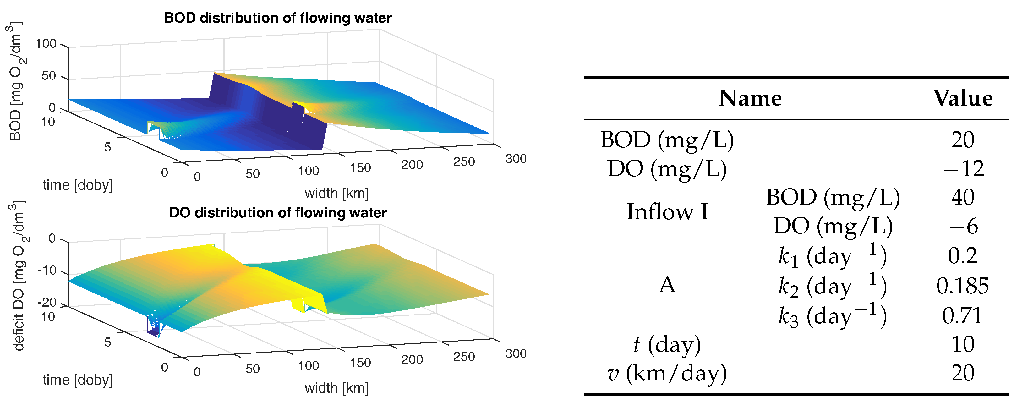
Hyper-surfaces for BOD and DO, which significantly reflect real river conditions (see

Table 3. Initial values for the spatial distribution of changes in BOD and DO.

BOD (mg/L)	DO (mg/L)	A			t (Day)	v (km/Day)
		${\mathit{k}}_1$ (Day${}^{-1})$	${\mathit{k}}_2$ (Day${}^{-1})$	${\mathit{k}}_3$ (Day${}^{-1})$
40	−5	0.2	0.185	0.71	10	20

), are the solution for the mathematical model with distributed parameters (6)–(8). Figure 13 presents BOD and DO distributions for steady edge conditions, BOD and DO values decrease over the course of time and length.

A further experiment concerned both the changeable initial and edge conditions occurring in the river. Real river conditions, such as variable initial conditions and occurrence of side pollution inflow variable in time were taken into consideration. The results and pre-assumed initial values of the parameters are shown in Figure 14. Extortions in the form of spikes in BOD and DO values were observed at the initial point of the analyzed river segment and at the time when the side inflow occurred. A sudden change of values remains for a particular period of time, and, after that, the values return to the previous state. In the considered BOD ad DO space-time distribution, the spikes which appear on the ”diagonal” decrease, which results from the river self-purification process. The pollution inflow variable in time causes the first pollution spike below the first inflow, which runs parallel to the second spike.

Speed has a significant influence on BOD and DO distribution. Carrying out experiment for various values of river speed, a different location of pollution spread against the time axis was observed in Figure 15:

It was observed that the placement of pollution “marks” changes accordingly with the increase of river flow speed. Therefore, the river speed is a crucial factor that causes variable placement of pollutants in rivers. The higher the river speed, the distance of the location of pollution concentration tends to increase. The self-purification process has too little time to reduce these values. The conducted studies showed little impact of the diffusion at equally high speeds of river flows. The diffusion was excluded from further considerations [32,34,52,53,54].

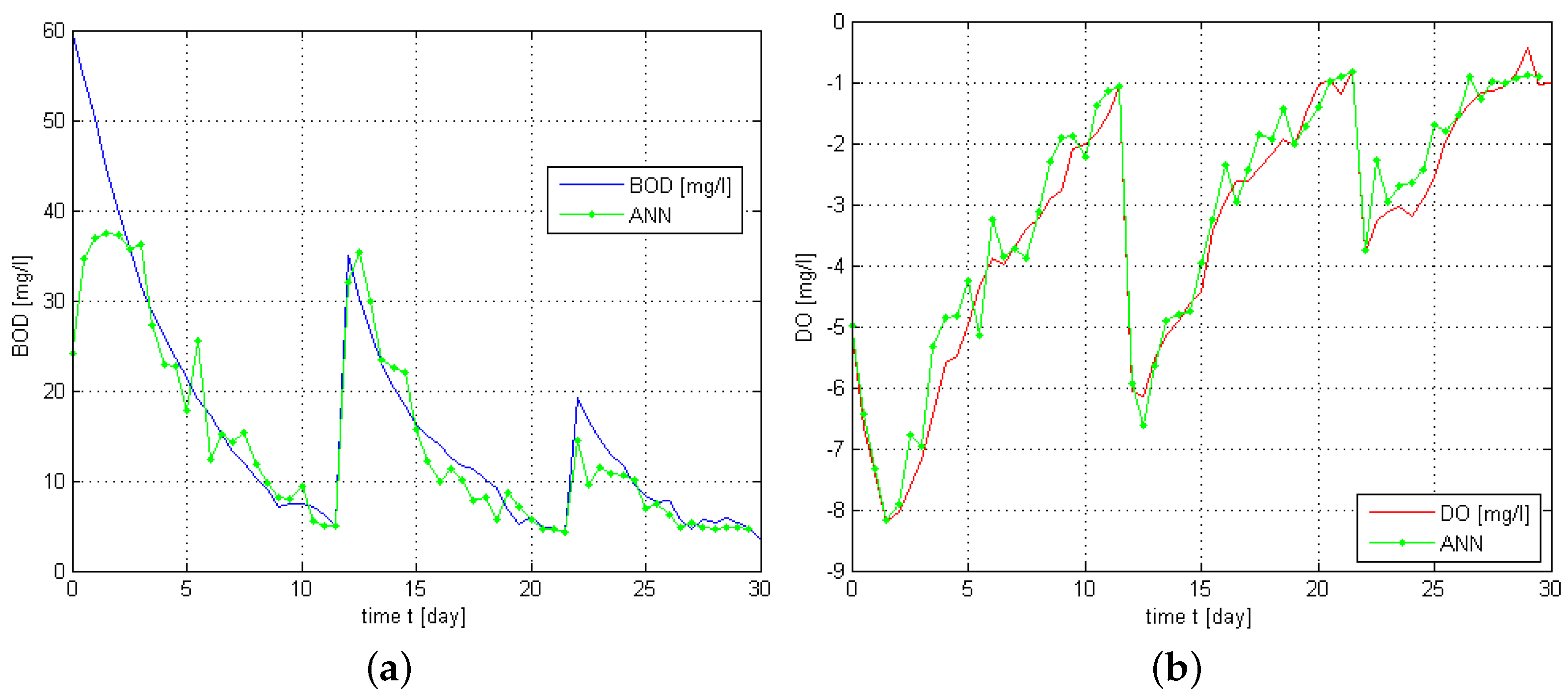
Using the proposed intelligent filtration and prediction module, a number of experiments were conducted for the investigated river object with two inflows. As a result BOD and DO distribution was obtained, which shows a correct ANN reaction to the introduced estimate value (Figure 16). As it can be observed, the values of estimates follow the BOD values. The training process has a significant influence on the accordance of estimates according to the expected courses. In extreme cases, the network significantly distorts estimates against their real values.

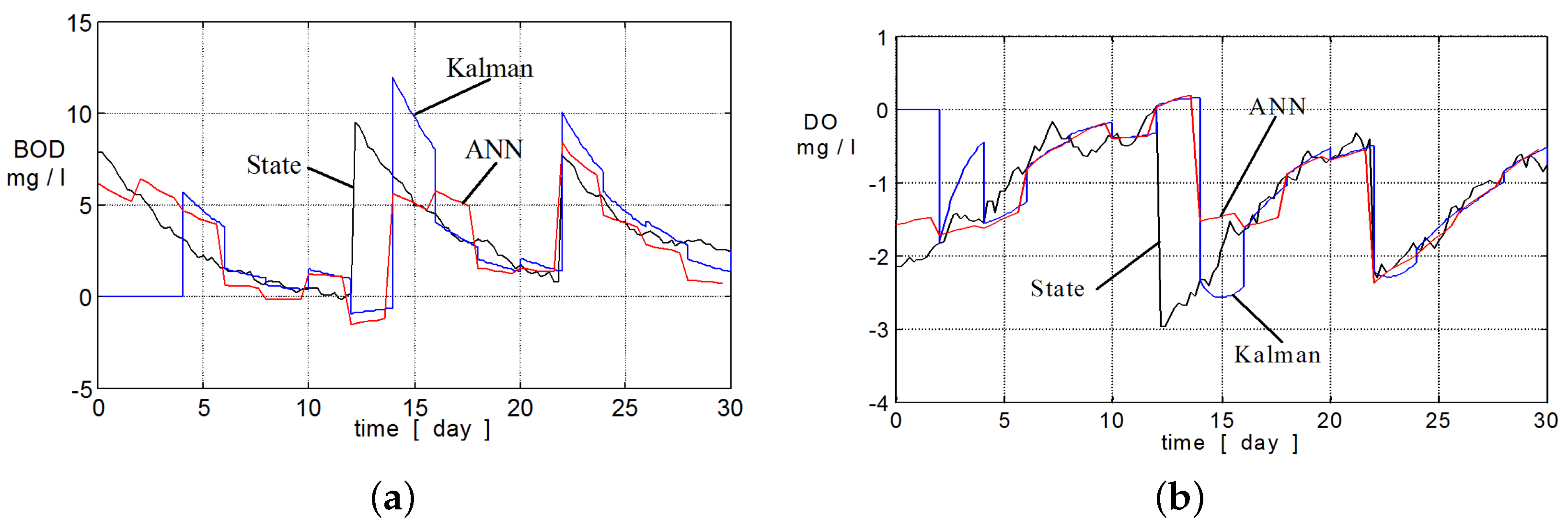
Using artificial neural network in the filtration and prediction phase improved the accuracy of estimation process. Net gives more precise estimates of river state than classical Kalman’s filter. It is easy to see from results of experiments that a neural network has also higher resistance to noises, changes of distance between measurement stations and leap changes of pollution indicators’ values (inflows). Moreover, applying the neural network allows a solution of knowledge of actual river parameters. It is hard to determine in practice. In addition, by proper selection of learning data on network answers can be improved in a specified range of pollution indicators values (Figure 17).

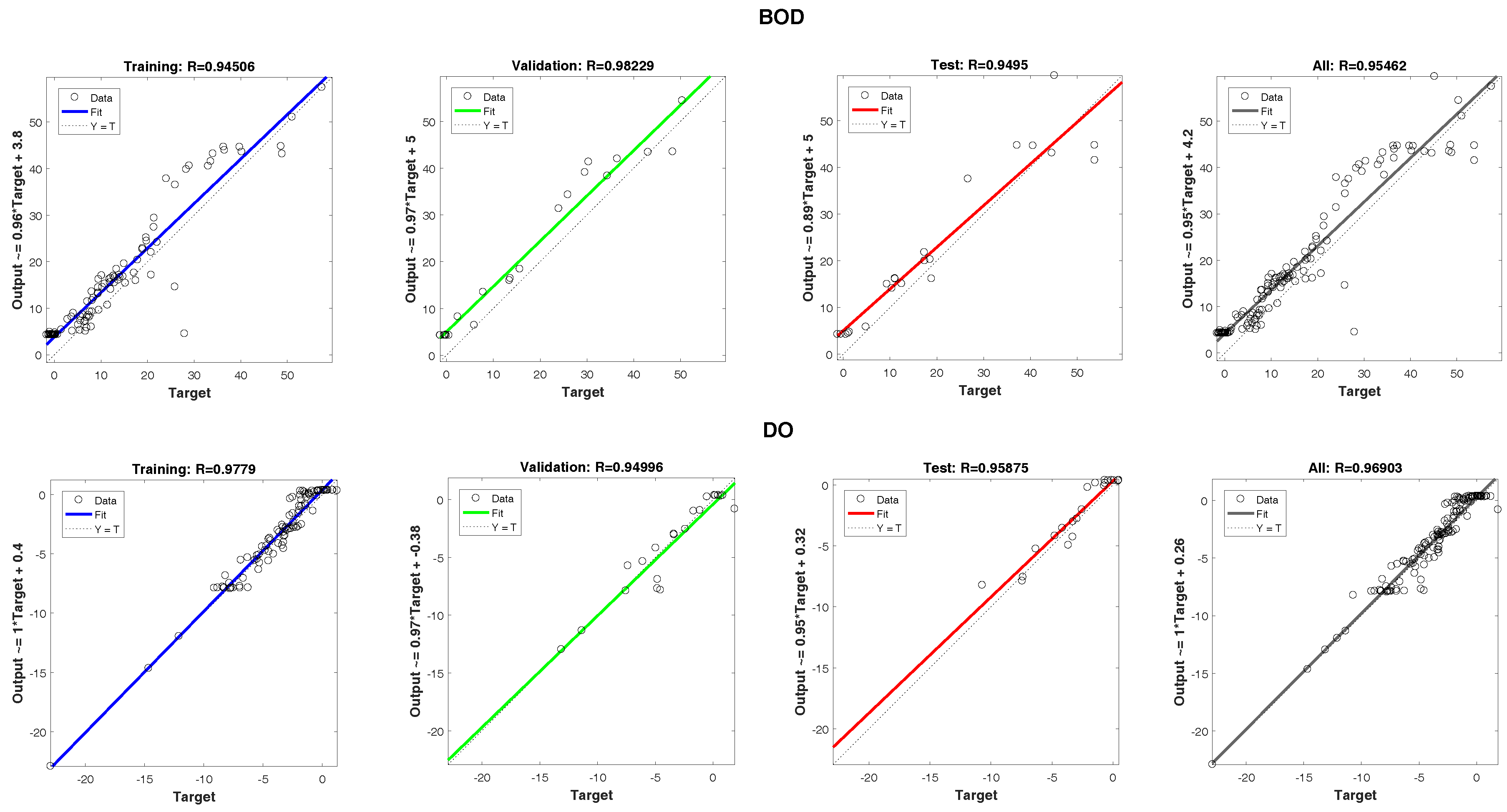
In Figure 18, plots representing the training, validation and testing data have been presented. The dashed line in each plot represents the perfect result − outputs = targets. The solid line represents the best fit linear regression line between outputs and targets. The R value is an indication of the relationship between the outputs and targets for BOD and DO, respectively. Training data indicates a relatively good fit of the ANN to river model. The validation and test results also show large R values. The scatter plots show the existence of several points badly fitted by ANN.

The quality indicator for comparison of the accuracy of estimation by Kalman’s filter and artificial neural network was applied as follows:

$$J=\sum _{i=t_0}^{t_k}\frac{{(X_i-\widehat{X_i})}^2}{n},$$

(47)

where X, $\widehat{X}$—state and estimate of river state, n—number of measurements. The mean squared error is the accepted standard indicator for the performance evaluation, which we applied to assess the proposed methods.

The obtained results, shown in the table above, encompasses quality coefficient values for six different configurations of the river model. The results confirm that artificial neural network gives more precise estimates of river state than classical Kalman’s filter. The quality indicators of BOD are greater because there is no information from measurements about that pollution indicator. Common analysis of Pearson coefficient (see Figure 19) and J indicator allows the assessment of the quality of the methods used. For DO, the Pearson index has values closer to 1, which implies that both methods achieved a similar performance level. On the other hand, for BOD, the lower values of the J (see

Table 4. Values of quality indicator for Kalman’s filter and neural network.

BOD		DO
Kalman’s Filter	ANN	Kalman’s Filter	ANN
12.338	4.306	0.571	0.553
12.984	4.693	0.615	0.610
11.262	3.702	0.553	0.533
3.233	0.158	0.141	0.103
3.789	2.470	0.149	0.111
3.675	2.511	0.176	0.132

) indicator and the Pearson coefficient clearly indicate the higher efficiency of ANN in relation to the Kalman filter in the estimation process.

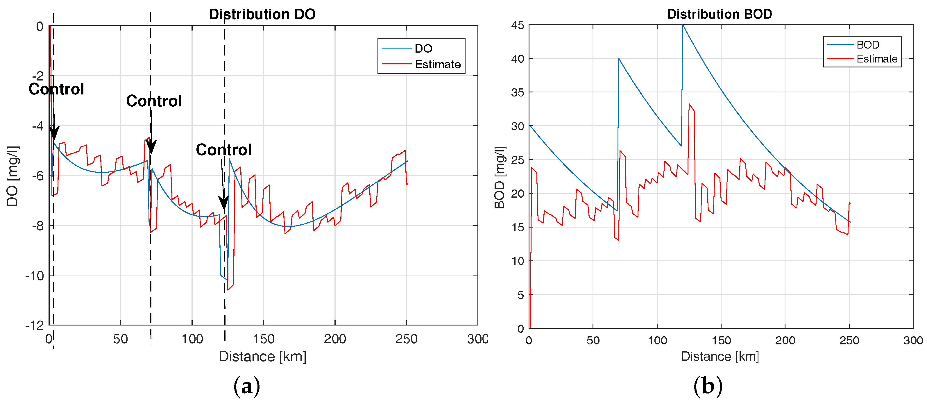
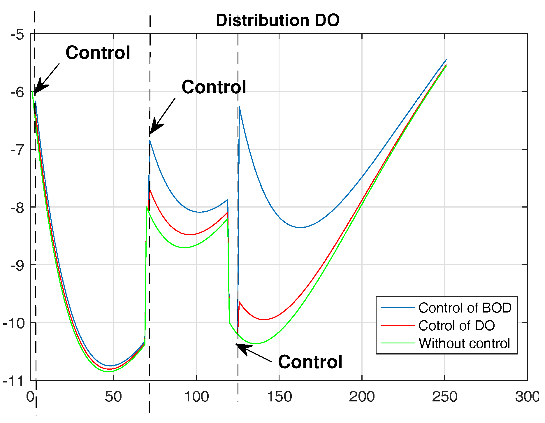
The river self-purification ability depends on biological processes that require a particular amount of oxygen. Calculating the control on the basis of DO deficit would appear to be easy and precise. Taking into consideration the character of the river processes, it may turn out to be insufficient as the ignorance of BOD may cause unexpectedly low DO values. A series of conducted studies included various conditions occurring in the river. Figure 20 shows a situation for the control including only DO indicator. The initial values of the parameters used in the experiments are shown in

Table 5. The initial values of the parameters.

Name		Value
BOD (mg/L)		30
DO (mg/L)		−5
A	$k_1$ (day${}^{-1})$	0.2
	$k_2$ (day${}^{-1})$	0.185
	$k_3$ (day${}^{-1})$	0.71
t (day)		10
v (km/day)		20
$k_{F1}$		−3.5
$k_{F2}$		1
$k_{p1}$		10
$k_{p2}$		5

, where: $k_{F1}$—filter gain coordinate for BOD, and $k_{F2}$—filter gain coordinate for DO. The values of coefficients $k_{F1}$, $k_{F2}$ (20) and $k_{p1}$, $k_{p2}$ (44) were determined on the basis of Riccati equations for the filter and for the regulator assuming experimentally selected values of elements of the matrices of $W_r$, V and R, P, respectively. These values were determined by means of actual measurements carried out for the Wislok River in years 2011–2015. Modification of the parameter values resulting from the hydrological profile of the river, and the obtained measurement accuracy resulting from the applied measuring devices has a key impact on the final quality of monitoring and control of water quality.

In the initial stage, DO deficit has low values and BOD high values. The control system that functions based on DO indicator does not fully react to the pollution as DO level is normal. Over the passage of time as a result of the increase in oxygen deficit caused by high BOD value, the system generates the control, but it may turn out that it is too late for an effective reaction—large deficits of DO still persist. The execution of control considering BOD indicator with a few days delay (laboratory service) is useless. The BOD indicator values in the proposed system are obtained from the estimation process. In order to precisely determine the amount of oxygen that is to be delivered to the body of water, the BOD estimate is used. Moreover, it is worth emphasizing that delivering too small or large amounts of oxygen is disadvantageous. The best solution is to calculate the controls based on BOD and DO indicator. On the basis of the current BOD values, too large of a DO deficit can be determined, and also precisely takes oxygen that must be introduced into the body of river. The conducted simulation studies are presented below.

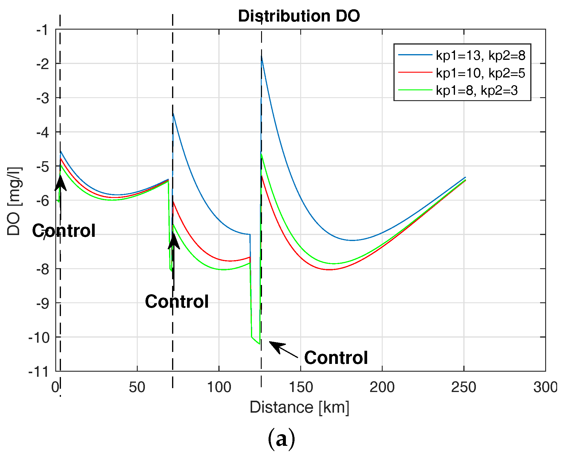
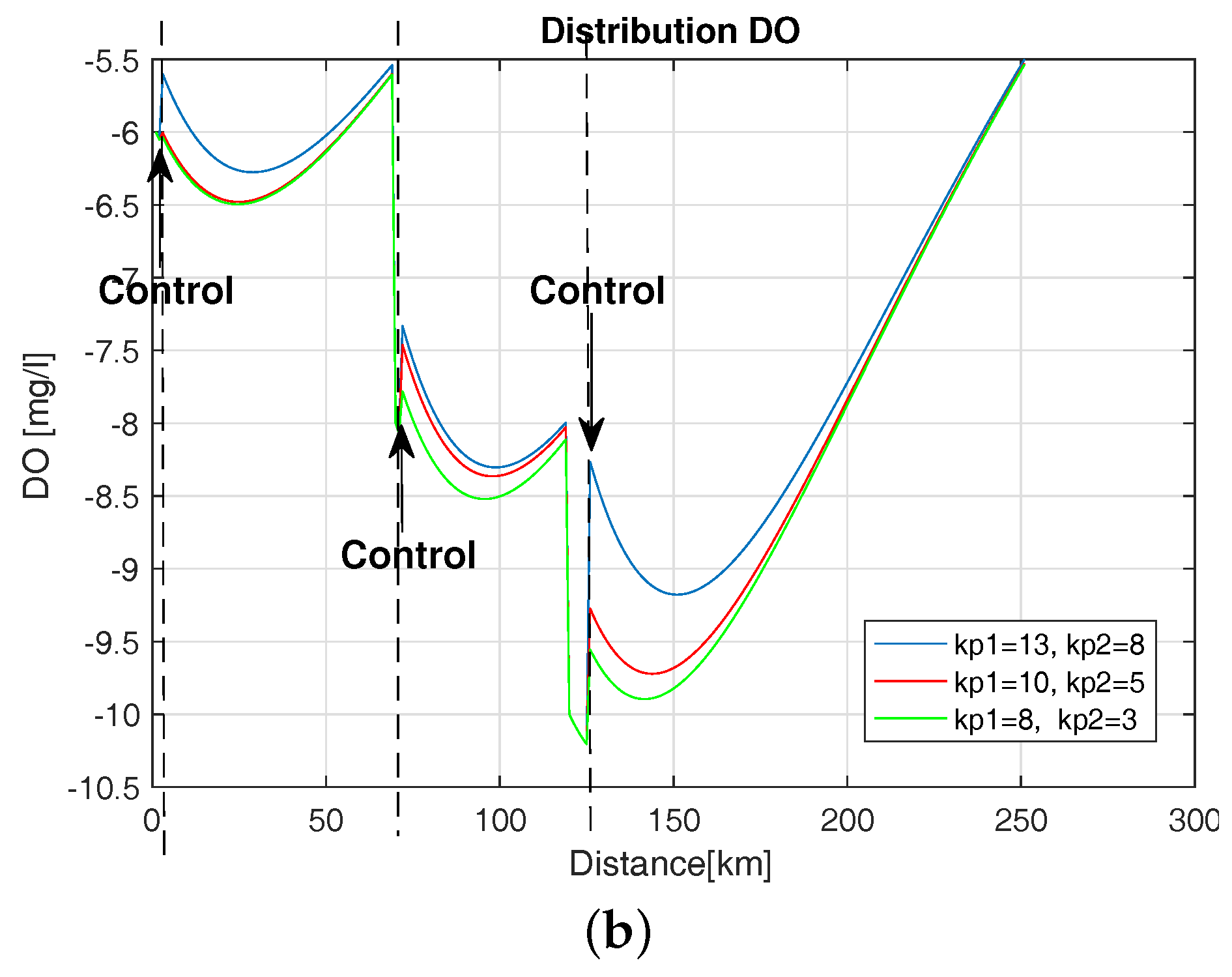
Introducing the control based on BOD and DO caused the system to react sufficiently early, which prevented the development of unfavorable conditions in the river and allowed the maintenance of DO values close to the assumed level. The experiments were carried out regarding various initial conditions for BOD and DO values and the influence of enhancement coefficients $k_{p1},k_{p2}$. Figure 21 shows the distribution of DO deficit with control for different values of $k_{p1}$ i $k_{p2}$ for initial conditions BOD = 30 (mg/L) and DO = −6 (mg/L). The control occurred in three places due to the occurrence of undesirable biological conditions in the river. Here, we see a significant influence of the value of the gain factor of the regulator. Small amplification values cause a lesser response to the change in DO during the control, leading to increased occurrence of hazardous conditions in the river.

The assumptions concerned the occurrence of large DO deficit at low BOD values and also a situation when high BOD values appear in the river at small DO deficit (Figure 22). The control system in the initial part of river segment based on DO indicator does not react to the appearing pollutants as DO level is normal. By contrast, the system reaction, based on both indicators, is observable at the very beginning of the river segment. As the distance and time pass, the oxygen deficit increases that threatens biological life in the water. When the pollutants inflow, the system reacts and improves the condition of water. The most satisfactory conditions in water are obtained during the use of BOD and DO control.

4. Conclusions

In the paper, the use of artificial neural networks to solve the problem represented by BOD and DO indicators has been presented. Neural networks were used to solve the problem of monitoring and controlling water quality in the river in real time. The analysis and control process was carried out using two BOD and DO indicators. The difficult–to-measure-in-real-time BOD indicator of water quality was estimated by ANN in real time, enabling monitoring of the river in real conditions. The above studies present a positive situation when the state estimation is used, especially when large amounts of pollutants occur in various places. Traditional process-based modeling methods concerning the biochemically polluted river control can provide less accurate estimations and predictions for water quality parameters represented by BOD and DO indicators. The conducted experiments with the use of ANN proved that the river pollution level control concerning both indicators generates better results than the control with the use of Kalman–Bucy filtering. Data generated by ANN for both indicators minimizes the occurrence of dangerous conditions in the river that can lead to an ecological disaster. Enhancement values are also significant during the control as they positively influence the course of biochemical pollution decomposition. Traditional models need data sets that require a long time to process and a large amount of input data that are often unknown. The use of the Kalman–Bucy filter is associated with the need to know many parameters of the river and especially the covariance of errors. In practice, it is difficult to estimate them, which leads to estimation errors. The determination of these parameters also requires a large amount of calculation. The ANN is a very effective technique that is capable of identifying complex nonlinear relationships between input and output data when compared to classical control technique based on Kalman–Bucy filter. In the paper, two approaches were proposed using ANN for the execution of estimation process. The former represents a separate network system for BOD and DO estimation while the latter concerns two neural networks that function in parallel. In both cases, correct results were achieved, but the second case was more universal. Because of the fact that water quality forecast can be simply affected by external environment, we observed that trained networks sometimes produced results that greatly deviated from the actual values. Therefore, further investigations needs to be conducted in future work to identify a more accurate forecast model. The observation of R coefficient values at consecutive stages of ANN training, validation and testing confirmed the efficient performance of the proposed intelligent filtration and prediction module. The obtained quality of BOD estimation by ANN in comparison to the quality of estimation obtained with the use of Kalman–Bucy filter shows the advantage of the first method. To estimate the ANN reliability level, we also performed network sensitivity tests by perturbing the BOD variable. The experiment has shown that the network output is sensitive to random changes of BOD concentrations. The amount of error increase reached 35% when the BOD concentrations has changed by 15%, while it reached only 6% when the BOD concentrations has changed by 8%. The obtained results of simulation studies allow the formulation of the main conclusion that it is possible to control the river aeration based on the measurements of particular state coordinates and the use of estimation process that completes the “knowledge” concerning unmeasured data. Although the comparison of ANN to the Kalman–Bucy filter shows the advantage of the former, in order to strengthen the objectivity of the quality assessment of the proposed system as a continuation of research, other indicators used in forecasting issues should be taken into account, e.g., the Nash–Sutcliffe efficiency coefficient, the median absolute percentage error, or the Persistence Index, recently proposed in works [11,14]. Another advantage of the proposed method concerns the ability of the system to simulate virtual states of river ecological condition without the risk of disaster in the actual subject. Of course, the ANN performance is limited by the range of the extrapolation effect obtained while learning the neural network. Based on the studies and observations, the authors state that it is possible to increase the accuracy of the adaptive BOD estimation mechanism. This effect can be achieved by extending the estimation error horizon by selecting the appropriate size of the time window. Information about the error rate history in the control system can increase the accuracy of the change in the value of the gain factor. The monitoring and control of a particular river segment with the proposed system will be significantly improved by expanding the monitoring infrastructure to the river inflows. This research work has managed to integrate several analytical and modeling methods that would prove to be useful for various institutions that are directly involved in the management of Wislok river water quality in the Carpathian mountains in the south of Poland.

References

1. Kuriata-Potasznik, A.; Szymczyk, S.; Skwierawski, A.; Glinska-Lewczuk, K.; Cymes, I. Heavy Metal Contamination in the Surface Layer of Bottom Sediments in a Flow-Through Lake: A Case Study of Lake Symsar in Northern Poland. Water 2016, 8. [Google Scholar] [CrossRef]
2. Namour, P.; Le Pimpec, P. Simulation of hyporheic self-purification in rivers: The assimilative capacity of proteins. Water Sci. Technol. 2001, 43, 231–238. [Google Scholar] [PubMed]
3. Streeter, H.W.; Phelps Earle, B. A Study of the Pollution and Natural Purification of the Ohio River; U.S. Department of Health, Education and Welfare: Washington, DC, USA, 1958.
4. Tang, C.; Hsieh, P. Dynamic Analysis of Vegetated Water Flows. J. Hydrol. Eng. 2016, 21. [Google Scholar] [CrossRef]
5. Siwek, K.; Osowski, S. Data mining methods for prediction of air pollution. AMCS Int. J. Appl. Math. Comput. Sci. 2016, 26, 467–478. [Google Scholar] [CrossRef]
6. Ucinski, D.; Patan, M. Sensor network design for the estimation of spatially distributed processes. AMCS Int. J. Appl. Math. Comput. Sci. 2010, 20, 459–481. [Google Scholar] [CrossRef]
7. Gomolka, Z.; Kwiatkowski, B.; Pekala, R. Noninvasive diagnosis of magnetising coil using artificial neural networks. Prz. Elektrotech. 2011, 87, 66–69. [Google Scholar]
8. Twarog, B.; Pekala, R.; Bartman, J.; Gomolka, Z. The changes of air gap in inductive engines as vibration indicator aided by mathematical model and artificial neural network. Discret. Contin. Dyn. Syst. 2007, 2007, 1005–1012. [Google Scholar]
9. Govindaraju, R. Artificial Neural Networks in Hydrology (II): Hydrologic Applications. J. Hydrol. Eng. 2000, 5, 124–137. [Google Scholar]
10. Gholami, V.; Chau, K.W.; Fadaee, F.; Torkaman, J.; Ghaffari, A. Modeling of groundwater level fluctuations using dendrochronology in alluvial aquifers. J. Hydrol. 2015, 529, 1060–1069. [Google Scholar] [CrossRef]
11. Wang, W.C.; Chau, K.W.; Xu, D.M.; Qiu, L.; Liu, C.C. The annual maximum flood peak discharge forecasting using Hermite projection pursuit regression with SSO and LS method. Water Resour. Manag. 2017, 31, 461–477. [Google Scholar] [CrossRef]
12. Taormina, R.; Chau, K.W.; Sivakumar, B. Neural network river forecasting through baseflow separation and binary-coded swarm optimization. J. Hydrol. 2015, 529, 1788–1797. [Google Scholar] [CrossRef]
13. Wu, C.L.; Chau, K.W.; Fan, C. Prediction of rainfall time series using modular artificial neural networks coupled with data-preprocessing techniques. J. Hydrol. 2010, 389, 146–167. [Google Scholar] [CrossRef]
14. Chen, X.Y.; Chau, K.W.; Busari, A.O. A comparative study of population-based optimization algorithms for downstream river flow forecasting by a hybrid neural network model. Eng. Appl. Artif. Intell. 2015, 46, 258–268. [Google Scholar] [CrossRef]
15. Chau, K.W.; Wu, C.L. A Hybrid Model Coupled with Singular Spectrum Analysis for Daily Rainfall Prediction. J. Hydroinform. 2010, 12, 458–473. [Google Scholar] [CrossRef]
16. Bartman, J.; Gomolka, Z.; Twarog, B. ANN training—The analysis of the selected procedures in Matlab environment. Monogr. Appl. Inform. Comput. Sci. Technol. 2015, 2015, 88–101. [Google Scholar]
17. Gomolka, Z.; Twarog, B.; Bartman, J.; Kwiatkowski, B. Improvement of Image Processing by Using Homogeneous Neural Networks with Fractional Derivatives Theorem. AIMS Discret. Contin. Dyn. Syst. 2011, 31, 505–514. [Google Scholar]
18. Gomolka, Z.; Dudek-Dyduch, E.; Kondratenko, Y.P. From Homogeneous Network to Neural Nets with Fractional Derivative Mechanism. In Lecture Notes in Computer Science, Proceedings of the Artificial Intelligence and Soft Computing (ICAISC 2017), Zakopane, Poland, 11–15 June 2017; Rutkowski, L., Korytkowski, M., Scherer, R., Tadeusiewicz, R., Zadeh, L., Zurada, J., Eds.; Springer: Cham, Switzerland, 2017; Volume 10245, pp. 52–63. [Google Scholar]
19. Kwater, T.; Pekala, R.; Krutys, P. The mathematical models of water pollution and interpretation of their distribution. Technol. News 2009, 1, 130–132. [Google Scholar]
20. Kwater, T.; Krutys, P.; Zeslawska, E. The quality of state estimation of measurements for model polluted river. Educ. Technol. Comput. Sci. 2014, 1, 611–616. (In Polish) [Google Scholar]
21. Pekala, R.; Krutys, P.; Zeslawska, E. Analysis and visualization of the Wislok river hydrological measurement. Technol. News 2012, 1, 16–19. [Google Scholar]
22. Kwater, T.; Krutys, P. Estimation of pollution of the river by artificial neural networks. Symbiosis Eng. Comput. Sci. 2010, 1, 37–66. [Google Scholar]
23. Basant, N.; Gupta, S.; Malik, A.; Singh, K. Linear and nonlinear modeling for simultaneous prediction of dissolved oxygen and biochemical oxygen demand of the surface water—A case study. Chemom. Intell. Lab. Syst. 2010, 104, 172–180. [Google Scholar] [CrossRef]
24. Dogan, E.; Sengorur, B.; Koklu, R. Modeling biological oxygen demand of the Melen River in Turkey using an artificial neural network technique. J. Environ. Manag. 2009, 90. [Google Scholar] [CrossRef] [PubMed]
25. Velasquez-Villada, C.; Donoso, Y. Delay/Disruption Tolerant Network-Based Message Forwarding for a River Pollution Monitoring Wireless Sensor Network Application. Sensors 2016, 16, 436. [Google Scholar] [CrossRef] [PubMed]
26. Yoshida, N.; Hoashi, J.; Morita, T. Improvement of a mediator-type biochemical oxygen demand sensor for on-site measurement. J. Biotechnol. 2001, 88, 269–275. [Google Scholar] [CrossRef]
27. El-Bestawy, E.; Hussein, H.; Baghdadi, H. Comparison between biological and chemical treatment of wastewater containing nitrogen and phosphorus. J. Ind. Microbiol. Biotechnol. 2014, 32, 195–203. [Google Scholar] [CrossRef] [PubMed]
28. Bahuguna, D.; Ujlayan, A.; Pandey, D.N. A comparative study of numerical methods for solving an integro-differential equation. Comput. Math. Appl. 2009, 57, 1485–1493. [Google Scholar] [CrossRef]
29. Fox, K. Water Treatment and Equipment Decontamination Techniques. J. Contemp. Water Res. Educ. 2004, 129, 18–21. [Google Scholar] [CrossRef]
30. Kasprzak, W. Adaptive computation metods in digital image sequence analysis. Prace Nauk. Politech. Warsz. Elektron. 2000, 127, 3–170. [Google Scholar]
31. Maleknejad, K.; Shahrezaee, M.; Khatami, H. Numerical solution of integral equations system of the second kind by block-pulse functions. Appl. Math. Comput. 2005, 166, 15–24. [Google Scholar] [CrossRef]
32. Thomas, E.; Jenkins, P.E. Aeration Control System Design: A Practical Guide to Energy and Process Optimization; John Wiley & Sons: Hoboken, NJ, USA, 2013. [Google Scholar]
33. Eom, K.H.; Lee, S.J.; Kyung, Y.S.; Lee, C.W.; Kim, M.C.; Jung, K.K. Improved Kalman Filter Method for Measurement Noise Reduction in Multi Sensor RFID Systems. Sensors 2011, 11, 10266–10282. [Google Scholar] [CrossRef] [PubMed]
34. Dippner, W. Mathematical modeling of the transport of pollution in water. Hydrol. Syst. Model. 2009, 2, 204–246. [Google Scholar]
35. Florensa, J.P.; Johannesa, J.; Van Bellegem, S. Identification and estimation by penalization in nonparametric instrumental regression. Econ. Theory 2011, 27, 472–496. [Google Scholar] [CrossRef]
36. Lee, E.; Dobbins, M.; DeCorby, K.; McRae, L.; Tirilis, D.; Husson, H. An optimal search filter for retrieving systematic reviews and meta-analyses. BMC Med. Res. Methodol. 2013, 12, 20–30. [Google Scholar] [CrossRef] [PubMed]
37. Bishop, C. Neural Networks for Pattern Recognition; Clarendon Press & Oxford University Press: Oxford, UK, 1996. [Google Scholar]
38. Plawiak, P.; Tadeusiewicz, R. Approximation of phenol concentration using novel hybrid computational intelligence methods. AMCS Int. J. Appl. Math. Comput. Sci. 2014, 24, 165–181. [Google Scholar] [CrossRef]
39. Tadeusiewicz, R.; Chaki, R.; Chaki, N. Exploring Neural Networks with C#; CRC Press, Taylor & Francis Group: Boca Raton, FL, USA, 2014. [Google Scholar]
40. Tadeusiewicz, R. Neural Networks in Mining Sciences—General Overview and Some Representative Examples. Arch. Min. Sci. 2015, 60, 971–984. [Google Scholar] [CrossRef]
41. Tadeusiewicz, R. Neural networks as a tool for modeling of biological systems. Bio-Algorithm. Med-Syst. 2015, 11, 135–144. [Google Scholar] [CrossRef]
42. Finotti, H.; Lenhart, S.; Van Phan, T. Optimal control of advective direction in reaction-diffusion population models. Am. Inst. Math. Sci. 2012, 1, 81–107. [Google Scholar] [CrossRef]
43. Gomolka, Z.; Twarog, B.; Zeslawska, E. Hand-written text segmentation and recognition within Matlab environment. Monogr. Appl. Inform. Comput. Sci. Technol. 2016, 2016, 72–87. [Google Scholar]
44. Jimeno-Sáez, P.; Senent-Aparicio, J.; Pérez-Sánchez, J.; Pulido-Velazquez, D.; Cecilia, J.M. Estimation of Instantaneous Peak Flow Using Machine-Learning Models and Empirical Formula in Peninsular Spain. Water 2017, 5, 347. [Google Scholar] [CrossRef]
45. Meng, C.; Zhou, J.; Tayyab, M.; Zhu, S.; Zhang, H. Integrating Artificial Neural Networks into the VIC Model for Rainfall-Runoff Modeling. Water 2016, 9, 407. [Google Scholar] [CrossRef]
46. Peng, T.; Zhou, J.; Zhang, C.; Fu, W. Streamflow Forecasting Using Empirical Wavelet Transform and Artificial Neural Networks. Water 2017, 5, 406. [Google Scholar] [CrossRef]
47. Qiao, J.; Hu, Z.; Li, W. Soft Measurement Modeling Based on Chaos Theory for Biochemical Oxygen Demand (BOD). Water 2016, 8, 581. [Google Scholar] [CrossRef]
48. Zhou, T.; Wang, F.; Yang, Z. Comparative Analysis of ANN and SVM Models Combined with Wavelet Preprocess for Groundwater Depth Prediction. Water 2017, 10, 781. [Google Scholar] [CrossRef]
49. Novak, M. Mathematical modelling and optimization of a waste water treatment plant by combined oxygen electrode and biological waste water treatment model. Appl. Math. Model. 2015, 36, 3813–3825. [Google Scholar] [CrossRef]
50. Pakshirajan, K.; Rene, E.R.; Ramesh, A. Biotechnology in Environmental Monitoring and Pollution Abatement 2015. BioMed Res. Int. 2015, 2015, 1–3. [Google Scholar] [CrossRef] [PubMed]
51. Dudek-Dyduch, E. Intelligent ALMM System for Discrete Optimization Problems—The Idea of Knowledge Base Application. In Advances in Intelligent Systems and Computing, Proceedings of the 38th International Conference on Information Systems Architecture and Technology (ISAT 2017), Szklarska Poręba, Poland, 17–19 September 2017; Wilimowska, Z., Borzemski, L., Świątek, J., Eds.; Springer: Cham, Switzerland, 2017; Volume 657. [Google Scholar]
52. Aniszewski, A. Mathematical modeling and practical verification of groundwater and contaminant transport in a chosen natural aquifer. Acta Geophys. 2009, 57, 435–453. [Google Scholar] [CrossRef]
53. Kloeden, P.E.; Lorenz, T. Pullback attractors of reaction-diffusion inclusions with space-dependent delay. Discret. Contin. Dyn. Syst. Ser. B 2017, 22, 1909–1964. [Google Scholar]
54. Chen, X.; Lam, K.Y.; Lou, Y. Dynamics of a reaction-diffusion-advection model for two competing species. Discret. Contin. Dyn. Syst. Ser. A 2012, 32, 3841–3859. [Google Scholar] [CrossRef]
Figure 1. Conceptual diagram of the river controlling and monitoring system.
Water 10 00004 g001
Figure 2. The i-th river segment diagram.
Water 10 00004 g002
Figure 3. Characteristics in space-time domain.
Water 10 00004 g003
Figure 4. Two-layer neural network of feed-forward type. I and K—length of input and output vector respectively, L—number of layers (2), Q—number of training pairs.
Water 10 00004 g004
Figure 5. Diagram of the monitoring and control system.
Water 10 00004 g005
Figure 6. Filtration and prediction system.
Water 10 00004 g006
Figure 7. Artificial neural network (ANN) in the filtration process.
Water 10 00004 g007
Figure 8. Artificial neural network in the prediction process.
Water 10 00004 g008
Figure 9. ANN in BOD and DO estimation process.
Water 10 00004 g009
Figure 10. Regulation system block diagram.
Water 10 00004 g010
Figure 11. BOD top, and DO graph bottom.
Water 10 00004 g011
Figure 12. Distribution of BOD and DO values taking into account the three lateral inflows.
Water 10 00004 g012
Figure 13. BOD (a) and DO (b) space-time distributions.
Water 10 00004 g013
Figure 14. BOD and DO distribution for various boundary conditions.
Water 10 00004 g014
NameValue
BOD (mg/L) 20
DO (mg/L) −12
Inflow IBOD (mg/L)40
DO (mg/L)−6
A k _ 1 (day 1 ) 0.2
k _ 2 (day 1 ) 0.185
k _ 3 (day 1 ) 0.71
t (day) 10
v (km/day) 20
Figure 15. BOD distribution for range of water flow speed.
Water 10 00004 g015
Figure 16. BOD (a) and DO (b) state and estimates, respectively.
Water 10 00004 g016
Figure 17. Estimation of BOD (a) and DO (b) obtained from Kalman’s filter and ANN.
Water 10 00004 g017
Figure 18. R values for the training, validation, testing and all data for BOD and DO indexes, respectively.
Water 10 00004 g018
Figure 19. Pearson correlation coefficient for BOD and DO quality indicators.
Water 10 00004 g019
Figure 20. BOD distribution and estimate (a); DO including the control from DO (b).
Water 10 00004 g020
Figure 21. DO distribution with BOD and DO control (a); DO distribution with DO control (b).
Water 10 00004 g021aWater 10 00004 g021b
Figure 22. Control for DO.
Water 10 00004 g022