Abstract
Tropical cyclone (TC) rainfall amounts are compared from 1950–2017 for Houston, Texas and Miami, Florida to estimate the risk of TC rain in both cities. Following the wake of Hurricanes Harvey and Irma in 2017, concern has risen over the future of raininess in these locations. Per-event rainfall amounts are aggregated using tracks taken from HURDAT, time-of-rain gathered from National Weather Service daily weather maps, and rainfall totals taken from airport monitoring stations. Risk analysis tools include descriptive statistics, time series, and return frequencies for Houston and Miami, and spatially interpolated surfaces for Hurricanes Harvey and Irma. The season duration is longer in Miami than in Houston. The uppermost rainfall events in the distribution for Houston show a significant increase through time, suggesting the most intense rainfall events are becoming worse for Houston. The expected return frequency for a Harvey-like event (940 mm) in Houston is every 230 years, on average, and the 90th percentile rain of 286 mm is expected once every 17 years (11–29; 90% significance). The expected return frequency for an Irene-like event (261 mm—maximum for location) in Miami is every 173 years, on average, and the 90th percentile rain of 167 mm is expected once every 11 years (7–17; 90% significance). Results show a substantial difference between Houston and Miami TC rainfall climatologies similar to the differences of Hurricanes Harvey and Irma. Though emergency management must be tailored for each TC, management for inland TC rainfall may be more applicable in Houston than in Miami.
Keywords:
hurricane; daily weather maps; extreme value theory; gulf of Mexico; risk; harvey; irma; 2017 1. Introduction
Hurricanes generate risk to the human environment in various ways. Some provide unprecedented depths of storm surge (Hurricane Katrina, 2005), while others are most impressive due to their violent winds (Hurricane Maria, 2017) [1,2,3] . Despite the risk, inland rainfall from TCs is understudied [4,5]. High amounts of inland rainfall can lead to widespread catastrophe, as was evidenced during Hurricane Harvey in Houston, Texas in 2017. Estimated damage costs total at $125 million and measured rainfall exceeded 50 inches [6]. Understanding rainfall from a tropical cyclone (TC) is difficult, because many TCs do not have homogenous rainfall at any given moment in time or throughout their lifetime. A greater understanding of this difference in per-event TC rainfall is needed.
The 2017 Atlantic hurricane season was the fifth-most active, costliest, and possibly third-deadliest season since official record keeping began for the North Atlantic in 1851 [7,8,9]. Two of the three strongest U.S. mainland hurricanes were Hurricane Harvey that made landfall near Houston, Texas on August 26 (wind speeds ≥ 60 ms) and Hurricane Irma that made landfall near Miami, Florida on September 10 (≥80 ms). During emergency response, Miami-Dade county in Florida experienced a full scale evacuation, a necessary effort due to expected severe winds from Irma, yet a similar evacuation was not called for in Houston during Harvey due to a lack of early organization in the TC. Before rapid intensification occurred, Houston’s mayor introduced concerns of 8.5 million people on the road during Harvey, and a lack of evacuation resulted in over 1000 people being rescued overnight after being trapped in their homes [10]. Recent studies show these rainfall impacts from TCs along coastlines will be more severe as an uncertain, warmer future approaches [11,12,13].
As with all TC events, the characteristics of Hurricanes Harvey and Irma were different, and each led to different effects in their respective cities. With respect to inland TC rainfall, most previous studies concentrate on satellite, modeled, or time-specific rainfall amounts [14,15,16,17]. Here, the focus for TC climatologies is based on per-event rainfall, similar to Knight and Davis [18]. Though Hurricanes Harvey and Irma were intense based on wind speed, they produced vastly different rainfall characteristics. Our study hypothesizes that the characteristics of Harvey and Irma, though different, may be indicative of the TC climatologies for Houston and Miami, and these TC climatologies may assist in future evacuation planning for each city.
To help minimize the TC rainfall research gap and, ideally, provide evidence for appropriate resource allocation for flood control, the differences in TC rainfall risk between Houston and Miami are considered. These cities are chosen as the main focal points due to the recent 2017 season and the arrivals of Harvey and Irma. Risk is defined as the statistical probability of occurrence and the interpreted results are applied to the individual cities. First, general seasonality of TC rainfall for both of the locations is discussed, followed by an analysis on the changing nature of TC rainfall over time. A return frequency analysis is applied to each location to estimate the expected type of TC rain event over a given time period. Finally, as an attempt to describe the varying nature of TC rainfall between Houston and Miami, Hurricanes Harvey and Irma, respectively, are used to showcase the estimated distribution of rainfall throughout the cities using spatial interpolation. Results presented below are supported by three main discussions: differences in ocean temperature, forward speed, and TC organization.
2. Materials and Methods
The study area for the following analyses is shown in Figure 1. Points are placed on the city centers of Houston (29.76 N, 95.37 W) and Miami (25.79 N, 80.32 W). Houston is situated on the northwest side of the Gulf of Mexico and is roughly 50 miles from the coast. According to the Census [19], Houston has a population of over 2 million people. Miami is situated on the eastern side of Florida, facing the Atlantic Ocean, with roughly 400,000 people directly on the coast.
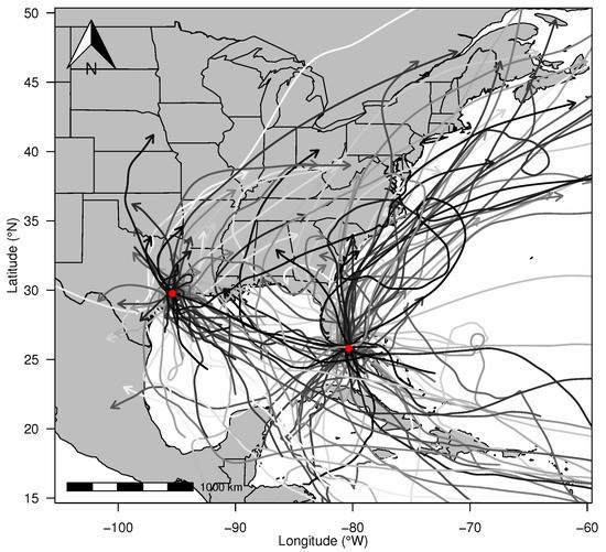
Figure 1.
Study Area with tropical cyclones (TCs) used in this study. Both locations are shown with points. Houston, Texas is near the northwest Gulf of Mexico and Miami, Florida faces the Atlantic Ocean. TCs are shaded based on their wind speed intensity at landfall: darker tracks indicate TCs with higher wind speeds.
2.1. Data
This study uses event-based analyses to calculate TC rainfall variability. Events were based on all measured rainfall from a given TC. Therefore, first, TCs for each city were compiled, then the lifetime of each TC was determined using Daily Weather Maps, and finally, rainfall totals from reliable weather stations were summed for each event. The data collection and procedures for analysis are discussed in the following subsections.
2.1.1. Tropical Cyclones
The National Hurricane Center provides an official record of U. S. -landfalling North Atlantic TCs in their Hurricane Database (HURDAT2; [20]). HURDAT2 consists of the six-hourly TC location and intensity data for 1851–present. Elsner and Jagger [21] provide a smoothing spline that interpolates, and preserves, those six-hour geographic position data to one-hour intervals. The one-hour interpolated tracks are considered the data source for identifying influencing TCs.
For this study, any TCs are included that may have produced rain for Houston or Miami. Keim et al. [22] show that major hurricanes (wind speeds ≥ 50 ms) can have TC force winds (≥18 ms) as far as 360 km wide. Recent studies also note the size of rain fields in landfalling TCs. Matyas [23] shows that U.S. landfalling hurricanes had average rain field extent of 223 km, and the average width of right and left sides for Gulf Coast landfalling hurricanes were 295 and 196 km, respectively [24]. Additionally, rain field size increased after landfall [24,25]. For this study, all TCs landfalling within 180 km of each city center are found using the computer program R to identify those events from HURDAT2. Reliable and complete rainfall data sets extend to 1950, so for the purposes of this study, all TCs influencing these cities from 1950–2017 are included. Note that HURDAT2 is not updated through 2017. Hurricanes Harvey (Houston) and Irma (Miami) were added to the data sets because rainfall data fromthose events are presently available as described below. Figure 1 shows the tracks influencing both cities (n = 37 and n = 68 for Houston and Miami respectively). The tracks are shaded to denote Saffir-Simpson scale wind speeds. The lightest tracks are those TCs with tropical storm wind intensity (≥18 ms) and the darkest tracks indicate TCs with Category 5 wind intensity (≥70 ms).
2.1.2. Daily Weather Maps
Hurricanes often produce continuous rainfall for longer than 24-h periods. To ensure that each rainfall event was truly from a hurricane, and to ensure that total rainfall from each hurricane was included, landfall dates were verified with Daily Weather Maps (DWMs) from the National Weather Service. The DWMs for Hurricane Claudette in 1979 is included as an example (Figure 2).
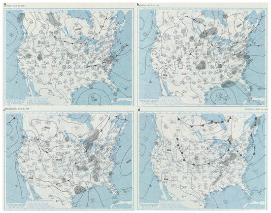
Figure 2.
Daily weather maps for Hurricane Claudette, 1979. (a) Sunday, 22 July, a low pressure zone moves in from the Gulf of Mexico. (b) Storm officially named Claudette. (c) Rainfall occurs for next three days. (d) The low pressure center leaves and stops bringing rain to Southeast Texas.
On Sunday, 22 July, a tropical low-pressure system forms in the Central Gulf of Mexico (Figure 2a). By the following day, the storm has formed a center of circulation with wind speeds greater than 18 ms, has moved northwestward, and the storm is named “CLAUDETTE” (Figure 2b). During the next three days, Hurricane Claudette hovers over Southeast Texas, and the DWMs indicate rainfall occurring at 7:00 a.m. EST in Houston for each of those days (Figure 2c). Finally, on Saturday, 28 July, the low pressure from Hurricane Claudette has weakened and moved to Northern Arkansas (Figure 2d). After tracking the hurricane with DWMs, it is catalogued that Hurricane Claudette possibly produced rain over six days (22–27 July). The final step references daily rainfall readings for the weather station at Houston Hobby Airport for the indicated days. Rainfall was recorded for each day during that period for a total of 292.86 mm (11.53 in).
2.1.3. Rainfall
The Southern Regional Climate Center housed at Louisiana State University provides climate data through its new, open-access CLIMDAT portal (climdata.srcc.lsu.edu). More than 40 stations are available within a 20-mile radius of the city centers of Houston and Miami. The closest and oldest reliable weather station for Houston is Hobby Airport, approximately 10 miles from the city center (1930–2018; 29.76 N, 95.37 W). Similarly, Miami’s oldest and most central weather station is its International Airport (1940–2018; 25.79 N, 80.32 W), also less than 10 miles from city center. Miami Beach is an older, closer weather station in Miami, but it did not record precipitation for Irma in 2017. Other stations are also available from each city, but they are farther from city center, contain more missing values, and do not significantly differ in values from the stations described above. Rainfall for each event was summed based on the inferences taken from the DWMs. For example, rainfall at Houston’s Hobby Airport for Hurricane Claudette was summed for 22–27 July (7.62 + 5.33 + 5.84 + 123.95 + 139.95 + 10.17 = 292.86 mm). This process was completed for each event.
Choosing the TCs, analyzing the daily weather maps, and aggregating the daily rainfall was completed for both of the cities. The final resulting data include 37 events for Houston and 68 events for Miami. Both data tables can be seen below in Table 1 and Table 2. The start day and end day for each TC correspond to the first time it was defined as a TC by the National Hurricane Center until it was no longer designated as a TC. Occasionally, the final day occurred in the subsequent month (e.g., Table 1, Hurricane Allison, 1989).

Table 1.
Tropical cyclone data used for Houston, Texas. Included are the storm name, year, month, start day (sDay), end day (eDay), and accumulated rainfall in mm.
Table 2.
Tropical cyclone data used for Miami, Florida. Included are the storm name, year, month, start day (sDay), end day (eDay), and accumulated rainfall in mm.
2.2. Risk Calculation
2.2.1. Time Series
To assess whether per event rainfall rates are increasing throughout the period of record (68 years), a time series analysis was conducted on each of the cities’ rainfall distributions. First, distributions were checked using the Shapiro-Wilks Test for Normality. An ordinary least-squares regression was initially used to establish a relationship between the independent variable, year, and the dependent variable, rainfall. A Yeo-Johnson transformation was used to transform the variables [26] when the residuals of the model were not normally distributed. Finally, a quantile regression was used to assess the upper-most rainfall events in the distribution [27]. Quantile regression is an extension of linear regression applied to quantiles of the dependent variable. A quantile is a point taken from the inverse cumulative distribution function so that the 0.9 quantile is the value such that 90% of the values are less than the value [28].
2.2.2. Extreme Value Return Periods
Extreme value theory (EVT) is a branch of statistics concerning models and analytical tools to understand the most rare event, as opposed to the typical or average event. It is similar to the central limit theorem by considering the limiting distributions of independent variables independent and identically distributed. A complete discussion of EVT is provided in Coles [29]. EVT allows the user to estimate return frequencies outside the known distribution of data. There are a variety of distributions falling under EVT, including the weibull, the frechet, and the gumbel. The distributions can be combined into the generalized extreme value (GEV) distribution. A GEV distribution fits the set of values consisting of a block maxima approach, that is, one peak event per year. Alternatively, EVT distributions can be used to create a two-parameter generalized Pareto distribution (GPD), allowing the user to keep all values exceeding a certain threshold. The threshold choice is a compromise between retaining enough TC rainfall amounts to estimate the distribution parameters with sufficient precision, but not too many that the rainfall distributions fail to be described by a GPD.
The following theorem discusses the GPD. Let be a sequence of independent random variables with a common distribution function F and let
Denote an arbitrary term in the sequence by X, and suppose that F satisfies, so that for large n, , the standard GEV equation applies for some , and . Then, for a large enough threshold, u, the distribution function of , conditional on , is approximately
defined on and , where and , and are the GEV parameters. Taking into account also the crossing rate of the threshold u gives a three-parameter model equivalent to the three-parameter GEV model [30]. Inference based on this GPD approach is generally superior because it relies on more data [30].
The functionality available in Elsner and Jagger [21] was used to estimate the return frequencies for TC rainfall in Houston and Miami. It is similar to the approaches offered in Malmstadt et al. [28], Trepanier [31], and Trepanier and Scheitlin [32]. Confidence intervals are provided using a bootstrap approach. The set of rainfall amounts are randomly sampled with replacement to create a bootstrap replicate. The model was run with this replicate and a new estimate of the return period was found. This procedure was run 1000 times and the upper and lower quantiles corresponding to specified probabilities are found.
2.2.3. Interpolated Surfaces
Hurricane rainfall was reliably recorded for Harvey in Houston at 18 stations, and at 12 stations in Miami for Irma. Using spatial interpolation, rainfall was estimated for Harvey across the counties of Houston and for Irma across Miami-Dade county. Kriging is used to estimate rainfall (z) at a given location. It is based on a weighted average of the z values over the entire domain where the weights are proportional to the spatial correlation Elsner and Jagger [21]. The estimates minimize the variance between the observed and interpolated values.
The spatial autocorrelation between the rainfall observation points is modeled first with a sample variogram. The sample variogram is given as
where is the number of distinct pairs of observation sites a lag distance h apart, and and are the rainfall totals at gauge sites i and j. The model assumes the rainfall field is stationary. The relationship between rainfall at two locations depends only on the relative positions of the sites and not on where the sites are located (i.e., refers to distance and orientation) [21]. The variogram provides a graphic showing the semivariance as a function of lag distance. From the sample variogram, the zero-lag semivariance, or nugget (), the partial sill (c), and the range (r) for the model are gathered. The equation defining the model curve over the set of lag distances h is
A model is then fit to the sample variogram. This variogram model is a mathematical relationship defining the semivariance as a function of lag distance. There are many model choices. For Houston, a Gaussian function is used as it fits the distribution of rain in Harvey best. For Miami, a Bessel function model is provided as well as a periodicity model. As noted in the results, rainfall in Irma is far more variable throughout Miami than Harvey in Houston. This is showcased in the interpolated surfaces of Miami.
3. Results
3.1. Comparing the Historical Record
There are 37 events included for Houston and 68 for Miami. Histograms for TC rainfall can be seen for Houston in Figure 3 and Miami in Figure 4. In both figures, events occurring in the last decade (post 2007) are shown in red to provide an indicator of temporal change. In both locations, the most recent events (i.e., within the last decade) do not always have the most intense rainfall amounts. This idea is further assessed in the following subsection. Both locations show non normal distributions with extremely long right tails indicating extreme distributions. In Houston, the majority of the events have rainfall below 250 mm, with an average of 116.43 mm. The peak occurred in Harvey in 2017 with a recorded 940.05 mm of rain. The lowest measurable rainfall occurred in Hurricane Debra in 1978 (2.29 mm). In Miami, the majority of the TCs produced rain less than 100 mm, with an average of 68.03 mm. The peak occurred in 1999 with the landfalling of Hurricane Irene (261.62 mm). The lowest measurable rainfall was 0.13 mm from an unnamed event in 1988. Histograms for the number of hours for each TC’s rainfall duration are also included in Figure 5 and Figure 6 for Houston and Miami, respectively. Most storms for both locations last fewer than 4 days, but the duration for TCs in Houston are nearly twice as long as those in Miami. From these numbers alone, it is easy to see the rainfall risk in Houston is higher than that of Miami.
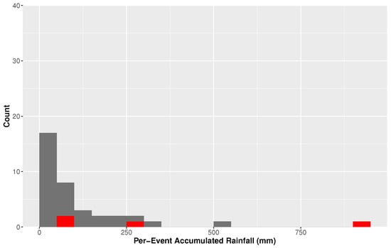
Figure 3.
Histogram for tropical cyclone rainfall for Houston, Texas. Red bars indicate events post 2007.
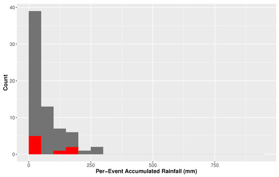
Figure 4.
Histogram for tropical cyclone rainfall for Miami, Florida. Red bars indicate events post 2007.
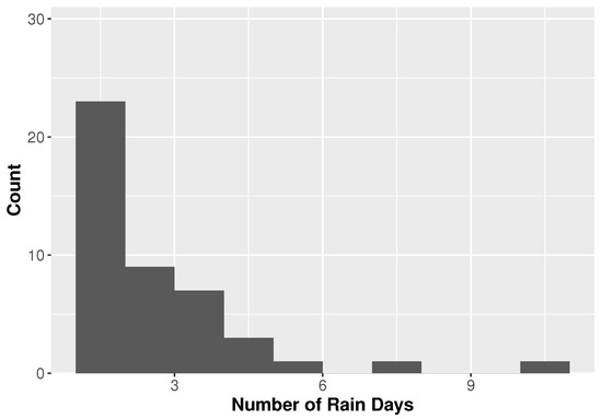
Figure 5.
Histogram for tropical cyclone rainfall duration for Houston, Texas.
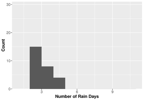
Figure 6.
Histogram for tropical cyclone rainfall duration for Miami, Florida.
The duration that a TC remains over a location may affect the amount of rainfall in an area. Figure 5 and Figure 6 show histograms for the number of hours that each TC produced rain for Houston and Miami, respectively. The majority of TCs at each location produce rainfall for fewer than 4 days at each location with a mean of and the largest number of TCs producing rain for no more than 48 h. However, the longest TCs in Houston last nearly twice as long as those in Miami.
The season for North Atlantic hurricanes runs from 1 June through 30 November. The seasonality varies depending on location. Figure 7 and Figure 8 showcase the monthly distributions of TC rainfall for Houston and Miami, respectively. The season is longer in Miami, with events occurring as early as February (note, this is prior to the official season start date) and as late as November. The February event was an unnamed event from 1952. The bulk of the Miami season begins in May with a peak in August, followed by September and October. The season dramatically slows down after October. In comparison, Houston has a much shorter TC season. The events begin in June and peak in September. After September, TC rainfall activity essentially diminishes. The risk of rainfall intensity seems to be higher in Houston, but the duration of risk is longer in Miami.
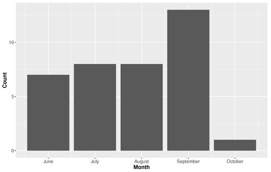
Figure 7.
Monthly distribution for tropical cyclone (TC) rainfall in Houston, Texas showcasing the seasonality of TC rainfall.
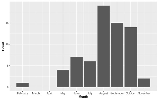
Figure 8.
Monthly distribution for tropical cyclone (TC) rainfall in Miami, Florida showcasing the seasonality of TC rainfall.
3.2. Changes Through Time
Research suggests changes in TC behavior may occur in a future climate due to warming temperatures from increased anthropogenic greenhouse gases [33,34]. In order to assess whether TC rainfall amounts are increasing or decreasing through time, a linear regression was used to model the relationship between year and rainfall at both locations. The initial linear models proved to be inadequate by violating assumptions of normality. After a Yeo-Johnson transformation to the variables, the relationships were successfully modeled and neither Houston or Miami show a significant trend in accumulated rainfall through time. Studies show the most extreme TC behavior is changing [35], so quantile regression was used to model the highest accumulated rainfall totals. Although only four events exist above 90th percentile of the rainfall data in Houston (283 mm), the confidence bounds of the model do not overlap zero, indicating positive, statistical significance. It is important to note this result is not robust with a sample size this small. However, it is interesting to discuss that the four events, Claudette in 1979, Allisons in 1989 and 2001, and Harvey in 2017 have all progressively increased through time. This suggests that the major events, when they do happen, produce more rainfall today than at the earliest part of the record. This is consistent with studies suggesting an increase in rain rates in present climatic conditions [33]. For Miami, a different relationship emerges from the model. A negative, insignificant relationship exists at all quantiles. Figure 9a shows the time series for Houston and Figure 9b shows the time series for Miami. Black lines are the modeled ordinary least squares relationships, and red lines are the modeled 90th percentile relationships.
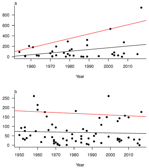
Figure 9.
Time series plots with year on the x-axis and accumulated rainfall amounts on the y-axis. Black lines indicate the ordinary least squares regression model and red lines are the models at the 90th percentile. (a) Houston, Texas. (b) Miami, Florida.
3.3. TC Return Frequency
Empirically, Houston receives rainfall from a TC every other year or so, with the number of TC rain events over the number of years in the record is roughly 0.57. Over the 67 year record, Houston experienced 37 events. In comparison, Miami receives one roughly every year, having 68 events over the 67 year period, an annual probability of 1.01. Both cities are modeled with thresholds set at the 60th percentile (Houston, 77.5 mm) and the 50th percentile (Miami, 43.1 mm). The threshold choice is a compromise between having enough rain events and having the distribution still be described by a GPD. These threshold choices are an adequate compromise. Using the EVT approach described above, the estimated return frequencies for the peak events in both locations were modeled using the GPD. Confidence bounds are provided using a bootstrapping procedure.
The model for Houston is shown in Figure 10. Annually, there is an 18.6% chance that rainfall from a TC in Houston will exceed the threshold of 77.5 mm. The curve shows two points, one for the 90th percentile of the rain distribution (286 mm) and one for Harvey at 940 mm. The confidence intervals about those points are shown with a red line. The model is far more successful modeling the 90th percentile than it is at modeling Harvey. Harvey’s rainfall amount is a major outlier for Houston, and its estimated return frequency is once every 230 years (90th CI: 96–Infinity). When modeling the 90th percentile, the expected return frequency for 286 mm of rain is once every 17 years, on average (11–29 years). The more reasonable confidence interval suggests a more robust model at this level.
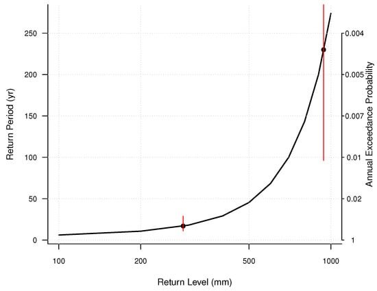
Figure 10.
Tropical cyclone rainfall return frequency for Houston, Texas. Return level in mm is shown on the x-axis, return period in years is shown on the y-axis. Annual probability is also included. Red lines about the points indicate confidence bounds at the 90th percentile. Points indicate the 90th percentile rainfall amount and Harvey in 2017.
The model for Miami is shown in Figure 11. Annually, there is an 38.5% chance that rainfall from a TC in Miami will exceed the threshold of 43.1 mm. The curve shows two points, one for the 90th percentile of the rain distribution (166.75 mm) and one for Hurricane Irene at 261.62 mm. The confidence intervals about those points are shown with a red line. Again, the model is far more successful modeling the 90th percentile than it is at modeling Hurricane Irene. The estimated return frequency for Hurricane Irene rainfall is once every 173 years (90th CI: 73–Infinity). When modeling the 90th percentile, the expected return frequency for 166.75 mm of rain is once every 11 years, on average (7–17 years). Note the x-axes on Figure 8 and Figure 9 are not the same, indicating the greater intensity risk in Houston.
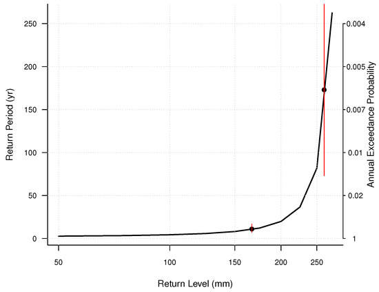
Figure 11.
Tropical cyclone rainfall return frequency for Miami, Florida. Return level in mm is shown on the x-axis, return period in years is shown on the y-axis. Annual probability is also included. Red lines about the points indicate confidence bounds at the 90th percentile. Points indicate the 90th percentile rainfall amount and Hurricane Irene in 1999.
3.4. Harvey and Irma
The final section of analysis provides interpolated rainfall surfaces of Hurricanes Harvey and Irma in Houston and Miami, respectively. It is to give an indication of the areas of the city hardest hit by rainfall amounts. The hope is individuals may look to these maps for comparison purposes when another storm approaches the shores. The background shapefiles for the counties surrounding Houston and Miami-Dade county are taken from the respective city government geographic information system portals available online.
Figure 12 shows the area surrounding Houston and the estimated rainfall based on 18 stations recorded rainfall during the event. The highest rainfall amounts occurred just to the southeast of Houston, with estimated measurements exceeding 1000 mm of rain. The northern parts of the city had slightly less rainfall, however totals still exceed 500 mm. The massive inundation of the greater area of Houston resulted in unprecedented losses for the state. The difference in distribution across the city led to different experiences, and, thus, presented a different risk to the individual. This is further explored in the discussion.
Figure 12.
Interpolated rainfall map for Houston, Texas during Hurricane Harvey 2017.
Figure 13 shows the two different models for the Miami area and the estimated rainfall based on 12 stations recorded rainfall during Irma. Figure 13a shows the Bessel model with a more linear representation, whereas Figure 13b shows the Periodic model which is obviously represented by the fluctuation in low and high precipitation amounts in Miami. Based on the data from Irma in Miami, the Periodic model seems to actually represent the distribution well. The meaning of these models is discussed in the following section in relation to the risk in Houston.
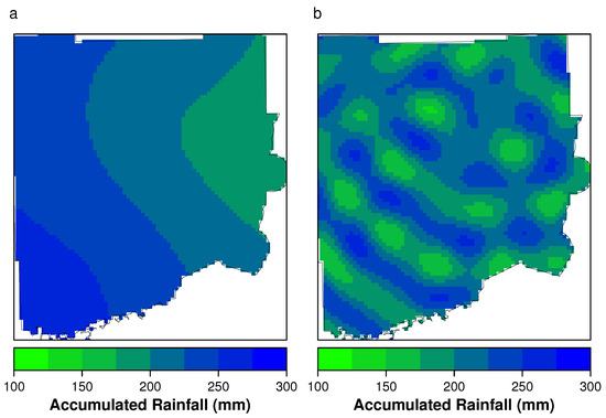
Figure 13.
Interpolated rainfall map for Miami, Florida during Hurricane Irma 2017. (a) Kriging model with Bessel variogram. (b) Kriging model with Periodic variogram.
4. Discussion
The approach here is to use event-based TC rainfall data, and as such, the number of events occurring at each location is important. During the same time interval, Miami received more TCs than Houston, likely due to its longer season of TCs. Miami’s positioning in the Atlantic basin leaves it open for TC landfall at almost any approach angle, whereas, TCs for Houston almost always come from the southeast [36]. The seasonality of TCs for Houston is also shorter than Miami, and the peak of the TC rainfall season is earlier in Miami when sea surface temperatures (SSTs) are lower. However, according to this study, the increased number of events and length of season for Miami does not increase its risk to TC rainfall. In fact, accumulated rainfall totals from TCs are nearly 50 percent greater in Houston than in Miami. The results of this study show that some characteristics of Hurricanes Harvey and Irma are also present in the full TC rainfall climatologies. We present some mechanisms to explain why these characteristics differ between the two sites, and we suggest that future research focus on the derth of knowledge within TC rainfall climatologies.
4.1. Possible Physical Mechanisms
This study suggests that TCs in the western Gulf of Mexico produce substantially different rainfall patterns than those in the eastern Gulf of Mexico. Based on limited previous research on TC rainfall, three mechanisms are suggested that may cause differences in TC rainfall pattern: (1) SSTs, (2) forward speed, and (3) TC organization.
Increased SSTs allow for Miami to have a longer season, but higher SSTs may cause a confounding effect on those TCs impacting Miami [37]. Rainfall from TCs in Houston averaged nearly 50 mm of rain more than in Miami. Miami is nearly surrounded on three sides by warm SSTs, whereas Houston only has one coastline. We suggest that similarly to previous storm surge research, differing coastline geomorphologies may impact the amount of rainfall on inland locations [38]. TC quadrants occurring over land typically have smaller rain fields and produce less rainfall [39]. Rainfall from Miami TCs may serendipitously occur over water instead of over land as a result of increased SSTs and available moisture.
Coastline geomorphology may also play a role in the forward speed of TCs. Previous models for TC rainfall note the importance of forward speed in rainfall, but few studies discuss its importance with respect to rainfall amounts [40,41]. Slower moving TCs are shown to produce more rain in a given area [42], and typically, TCs move more quickly at lower latitudes [43]. However, for this study, the majority of TCs impacting Houston moved at slower speeds than those impacting Miami, ultimately causing a longer duration of rainfall for most TCs in Houston. We suggest that the largest land mass surrounding Houston provides increased friction to TCs, and TC forward speed must slow down. As a result, the same amount of rainfall occurs over a shorter distance, thus producing more rainfall for a local area. Additionally, a TC path that recurves sharply may have a larger impact on a smaller spatial area. Figure 1 shows that storms do recurve more sharply in Houston than in Miami. Future research should further analyze the climatology of TC forward speed and shape of TC storm track in the Atlantic hurricane basin.
Finally, TCs in the western Gulf of Mexico often fragment and disperse more so than TCs in the eastern Gulf of Mexico [44]. Though this study alone cannot corroborate TC shape-rainfall relationship, these results suggest that a TC rainfall dichotomy exists between the eastern and western Gulf of Mexico. We suggest that future research concentrate on TC compactness with event-based TC rainfall data to support the following hypothesis: though an organized TC may be more intense in terms of wind or storm surge, an unorganized TC may bring more local rainfall to site-specific areas as rain bands split off from the center and form their own localized convection.
4.2. TC Return Frequency
Previous studies show that the most intense TCs are becoming more intense with time [33,45]. This study corroborates observations in the literature with respect to the most intense rainfall for Houston, TX. Extreme TC rainfall for Houston comes in the form of slow-moving, less organized TCs. These TCs often produce large amounts of rainfall over a singular, local area, and, likely as a result of increasing global SSTs, the localized rain fields have become more intense. However, Miami does not show a similar pattern. The increasing intensity of Miami TCs is not being manifested in rainfall amounts like it is in Houston.
TCs falling within the 90th percentile for rainfall are successfully modeled by this study. However, the largest rainfall-producing TC events, such as Harvey, are often difficult to predict. Although Harvey is a major outlier, TCs in Houston usually produce more rainfall than those in Miami. The return period for 90th percentile rainfall in Houston is longer than Miami, but Houston’s 90th percentile rainfall amount is more than 100 mm greater than Miami’s. The higher probability for a greater magnitude rainfall event in Houston should provide evidence for appropriate resource allocation. Inland flooding protection resources will likely have a greater effect on saving lives and infrastructure in Houston than in Miami, all else being equal.
4.3. Hurricanes Harvey and Irma
The 2017 TCs impacting Houston and Miami were indicative of their climatologies described previously. As an example, we have chosen Hurricanes Harvey and Irma to show this comparison (Figure 10 and Figure 11). Harvey had a distinct bias of rainfall to the southeast of the city center. TC rainfall interacted with storm surge and high wind speeds to flood the largest oil refinery in the United States in Beaumont, TX in the area of greatest rainfall. Harvey’s forward speed slowed to less than 2 mph at times, and its northeast quadrant was centered over Southeast Houston, where it could gather moisture from the warm Gulf of Mexico for a long period of time. The intense amount and longer duration of rainfall from Harvey contrast that of Irma and these similarities also exist in the TC rainfall climatologies at each landfall location.
Contrast these results to Irma, another strong TC that stayed organized, traveled quickly, and produced modest rainfall for Miami. Figure 13 shows two interpolations for Irma rainfall in Miami, and neither interpolation showed strong agreement to any distinct rainfall pattern. The periodic variogram (Figure 13b) actually produced an interpolation most similar to empirical values from Miami. We suggest that the Periodic variogram works well because the rainfall from Irma was comparatively consistent over its path, and it may represent the multiple rain bands common in a more organized TC. Lastly, note the differences in scale between the two events: the highest rainfall values for Irma in Miami are half that of even the lowest values for Harvey in Houston.
5. Conclusions
This paper was written as an attempt to quantify the differences in per-event TC rainfall risk between Houston, Texas and Miami, Florida. The purpose is two-fold. First, the paper aims to expand the literature on the geographic differences in hurricane risk. As numerical models are being built and forecasts being interpreted, the geographic variability of the results needs to be considered. Not all locations experience the same type of risk. The relative risk of an event becomes increasingly important to understand. The procedures described here are an attempt at showcasing this geographic variability and could be considered useful for similar types of comparisons. Second, the results implicate Houston has a greater risk of more extreme rainfall than Miami.
It is likely Miami would not experience rainfall amounts rivaling Hurricane Harvey in Houston. Miami experiences more events, but they are not as extreme as those experienced by Houston. This means Houston’s large population of 2 million people is arguably more at risk for extreme TC rainfall events than the population of Miami. This suggests funding for mitigation efforts regarding inland floodwaters should be focused more on Southeast Texas than on the eastern shores of Florida. The greater risk and greater population of Houston provide a location where mitigation and protection efforts could be increased and the lives and money saved could be exponential.
Author Contributions
J. C. Trepanier and C. S. Tucker designed the project. Tucker gathered the necessary data. Trepanier created the code in the open-source software, R, to statistically model the observations. Trepanier and Tucker analyzed the results and wrote the paper.
Acknowledgments
The authors would like to acknowledge the Fellowship received through the National Academies of Sciences, Engineering, and Medicine Gulf Research Program, with Sponsor Award Reference Number 2000007267. The fellowship provided through this program provided funds to allow this work to happen. The authors would also like to acknowledge the hard work of the reviewers and editor. Their contribution made this a stronger body of work.
Conflicts of Interest
The authors declare no conflict of interest. The funding sponsors had no role in the design of the study; in the collection, analyses, or interpretation of data; in the writing of the manuscript, and in the decision to publish the results.
References
- Feng, Y.; Negron-Juarez, R.I.; Patricola, C.M.; Collins, W.D.; Uriarte, M.; Hall, J.S.; Clinton, N.; Chambers, J.Q. Rapid remote sensing assessment of impacts from Hurricane Maria on forests of Puerto Rico. Peer J. Prepr. 2018. [Google Scholar] [CrossRef]
- Lin, L.; Weng, F. Estimation of hurricane maximum wind speed using temperature anomaly derived from advanced technology microwave sounder. IEEE Geosci. Remote Sens. Lett. 2018, 15, 639–643. [Google Scholar] [CrossRef]
- Jonkman, S.N.; Maaskant, B.; Boyd, E.; Levitan, M.L. Loss of life caused by the flooding of New Orleans after Hurricane Katrina: Analysis of the relationship between flood characteristics and mortality. Risk Anal. 2009, 29, 676–698. [Google Scholar] [CrossRef] [PubMed]
- Emanuel, K.; Ravela, S.; Vivant, E.; Risi, C. A statistical deterministic approach to hurricane risk assessment. Bull. Am. Meteorol. Soc. 2006, 87, 299–314. [Google Scholar] [CrossRef]
- Langousis, A.; Veneziano, D. Long-term rainfall risk from tropical cyclones in coastal areas. Water Resour. Res. 2009, 45. [Google Scholar] [CrossRef]
- NOAA (National Oceanic and Atmospheric Administration) Office for Coastal Management. Hurricane Costs. 2018. Available online: https://coast.noaa.gov/states/fast-facts/hurricane-costs.html (accessed on 27 April 2018.).
- Halverson, J.B. The Costliest Hurricane Season in US History. Weatherwise 2018, 71, 20–27. [Google Scholar] [CrossRef]
- Rivera, R.; Rolke, W. Estimating the death toll of Hurricane Maria. Significance 2018, 15, 8–9. [Google Scholar] [CrossRef]
- Klotzbach, P.J.; Bowen, S.G.; Pielke, R., Jr.; Bell, M. Continental United States hurricane landfall frequency and associated damage: Observations and future risks. Bull. Am. Meteorol. Soc. 2018. [Google Scholar] [CrossRef]
- Andone, D. Houston Knew It Was at Risk of Flooding, so Why Didn’t the City Evacuate? Online Newspaper. 2017. Available online: https://edition.cnn.com/2017/08/27/us/houston-evacuation-hurricane-harvey/index.html (accessed on 2 May 2018).
- Mori, N.; Kjerland, M.; Nakajo, S.; Shibutani, Y.; Shimura, T. Impact assessement of climate change on coastal hazards in Japan. Hydrol. Res. Lett. 2016, 10, 101–105. [Google Scholar] [CrossRef][Green Version]
- Takemi, T.; Okada, Y.; Ito, R.; Ishikawa, H.; Nakakita, E. Assessing the impacts of global warming on meteorological hazards and risks in Japan: Philosophy and achievements of the SOUSEI program. Hydrol. Res. Lett. 2016, 10, 119–125. [Google Scholar] [CrossRef]
- Cheung, K.; Yu, Z.; Eisberry, R.L.; Bell, M.; Jiang, H.; Lee, T.C.; Lu, K.; Oikawa, Y.; Qi, L.; Rogers, R.F.; et al. Recent advances in research and forecasting of tropical cyclone rainfall. Trop. Cyclone Res. Rev. 2018, 7, 106–127. [Google Scholar]
- Englehart, P.J.; Douglas, A.V. The role of eastern North Pacific tropical storms in the rainfall climatology of western Mexico. Int. J. Climatol. 2001, 21, 1357–1370. [Google Scholar] [CrossRef]
- Rodgers, E.B.; Adler, R.F.; Pierce, H.F. Contribution of tropical cyclones to the North Atlantic climatological rainfall as observed from satellites. J. Appl. Meteorol. 2001, 40, 1785–1800. [Google Scholar] [CrossRef]
- Marks, F.; Kappler, G.; DeMaria, M. Development of a Tropical Cyclone Rainfall Climatology and Persistence (RCLIPER) Model. In Proceedings of the 25th Conference on Hurricanes and Tropical Meteorology, San Diego, CA, USA, 29 April–3 May 2002; American Meteor Society: Boston, MA, USA; pp. 327–328. [Google Scholar]
- Shepherd, J.M.; Grundstein, A.; Mote, T.L. Quantifying the contribution of tropical cyclones to extreme rainfall along the coastal southeastern United States. Geophys. Res. Lett. 2007, 34. [Google Scholar] [CrossRef]
- Knight, D.B.; Davis, R.E. Climatology of tropical cyclone rainfall in the southeastern United States. Phys. Geogr. 2007, 28, 126–147. [Google Scholar] [CrossRef]
- Census, U.S. Interactive Population Map; Technical report; United States Census Bureau: Suitland, MD, USA, 2010. [Google Scholar]
- Landsea, C.; Franklin, J.; Beven, J. The Revised Atlantic Hurricane Database (HURDAT2); Technical report; National Hurricane Center: Miami, FL, USA, 2015. [Google Scholar]
- Elsner, J.B.; Jagger, T.H. Hurricane Climatology: A Modern Statistical Guide Using R; Oxford University Press: New York, NY, USA, 2013; p. 430. [Google Scholar]
- Keim, B.; Muller, R.; Stone, G. Spatiotemporal patterns and return periods of tropical storm and hurricane strikes from Texas to Maine. J. Clim. 2007, 20, 3498–3509. [Google Scholar] [CrossRef]
- Matyas, C.J. Associations between the size of hurricane rain fields at landfall and their surrounding environments. Meteorol. Atmos. Phys. 2010, 106, 135–148. [Google Scholar] [CrossRef]
- Zhou, Y.; Matyas, C.J. Spatial characteristics of storm-total rainfall swaths associated with tropical cyclones over the Eastern United States. Int. J. Climatol. 2017, 37, 557–569. [Google Scholar] [CrossRef]
- Matyas, C.J.; Guo, Q. Comparing the spatial extent of Atlantic basin tropical cyclone wind and rain fields prior to land interaction. Phys. Geogr. 2016, 37, 5–25. [Google Scholar]
- Kwon Yeo, I.; Johnson, R.A. A new family of power transformations to improve normality or symmetry. Biometrika 2000, 87, 954–959. [Google Scholar]
- Koenker, R.; Bassett, G. Regression quantiles. Econometrica 1978, 46, 33–50. [Google Scholar] [CrossRef]
- Malmstadt, J.; Elsner, J.; Jagger, T. Risk of strong hurricane winds to Florida cities. J. Appl. Meteorol. Climatol. 2010, 49, 2121–2132. [Google Scholar] [CrossRef]
- Coles, S. An Introduction to Statistical Modeling of Extreme Values; Springer: Berlin, Germany, 2001; p. 208. [Google Scholar]
- Coles, S.; Powell, E. Bayesian methods in extreme value modelling: A review and new developments. Int. Stat. Rev. 1996, 64, 119–136. [Google Scholar] [CrossRef]
- Trepanier, J.C. Hurricane winds over the North Atlantic: Spatial analysis and sensitivity to ocean temperature. Nat. Hazards 2014. [Google Scholar] [CrossRef]
- Trepanier, J.C.; Scheitlin, K.N. Hurricane wind risk in Louisiana. Nat. Hazards 2014, 70, 1181–1195. [Google Scholar] [CrossRef]
- Knutson, T.; McBride, J.; Chan, J.; Emanuel, K.; Holland, G.; Landsea, C.; Held, I.; Kossin, J.; Srivastava, A.; Sugi, M. Tropical cyclones and climate change. Nat. Geosci. 2010. [Google Scholar] [CrossRef]
- Zhang, L.; Karnauskas, K.B.; Donnelly, J.P.; Emanuel, K. Response of the North Pacific tropical cyclone climatology to global warming: Application of dynamical downscaling to CMIP5 models. J. Clim. 2017, 30, 1233–1243. [Google Scholar] [CrossRef]
- Elsner, J.; Kossin, J.; Jagger, T. The increasing intensity of the strongest tropical cyclones. Nature 2008, 455, 92–95. [Google Scholar] [CrossRef] [PubMed]
- Scheitlin, K.N.; Mesev, V.; Elsner, J.B. Polyline averaging using distance surfaces: A spatial hurricane climatology. Comput. Geosci. 2013, 52, 126–131. [Google Scholar] [CrossRef]
- Trepanier, J.C.; Ellis, K.N.; Tucker, C.S. Hurricane risk variability along the Gulf of Mexico Coastline. PLoS ONE 2015, 10, e0118196. [Google Scholar] [CrossRef] [PubMed]
- Bilskie, M.V.; Hagen, S.; Alizad, K.; Medeiros, S.; Passeri, D.; Needham, H.; Cox, A. Dynamic simulation and numerical analysis of hurricane storm surge under sea level rise with geomorphologic changes along the northern Gulf of Mexico. Earth’s Future 2016, 4, 177–193. [Google Scholar] [CrossRef]
- Matyas, C.; Srinivasan, S.; Cahyanto, I.; Thapa, B.; Pennington-Gray, L.; Villegas, J. Risk perception and evacuation decisions of Florida tourists under hurricane threats: A stated preference analysis. Nat. Hazards 2011, 59, 871–890. [Google Scholar] [CrossRef]
- Rego, J.L.; Li, C. On the importance of the forward speed of hurricanes in storm surge forecasting: A numerical study. Geophys. Res. Lett. 2009, 36. [Google Scholar] [CrossRef]
- Lonfat, M.; Rogers, R.; Marchok, T.; Marks, F.D., Jr. A parametric model for predicting hurricane rainfall. Mon. Weather Rev. 2007, 135, 3086–3097. [Google Scholar] [CrossRef]
- Elsner, J.; Kara, A. Hurricanes of the North Atlantic: Climate and Society; Oxford University Press: Oxford, UK, 1999; p. 488. [Google Scholar]
- Davidson, R.A.; Lambert, K.B. Comparing the hurricane disaster risk of US coastal counties. Nat. Hazards Rev. 2001, 2, 132–142. [Google Scholar] [CrossRef]
- Zick, S.E.; Matyas, C.J. A shape metric methodology for studying the evolving geometries of synoptic-scale precipitation patterns in tropical cyclones. Ann. Am. Assoc. Geogr. 2016, 106, 1217–1235. [Google Scholar] [CrossRef]
- Elsner, J.B.; Jagger, T.; Niu, X.F. Changes in the rates of North Atlantic major hurricane activity during the 20th century. Geophys. Res. Lett. 2000, 27, 1743–1746. [Google Scholar] [CrossRef]


© 2018 by the authors. Licensee MDPI, Basel, Switzerland. This article is an open access article distributed under the terms and conditions of the Creative Commons Attribution (CC BY) license (http://creativecommons.org/licenses/by/4.0/).