Article

Clouds over East Asia Observed with Collocated CloudSat and CALIPSO Measurements: Occurrence and Macrophysical Properties

1
Key Laboratory of Atmospheric Optics, Chinese Academy of Sciences, Hefei 230031, China
2
Brookhaven National Laboratory, Upton, NY 11973, USA
3
China Mobile Group Design Institute Co., Ltd., Beijing 100038, China
*
Author to whom correspondence should be addressed.
Atmosphere 2018, 9(5), 168; https://doi.org/10.3390/atmos9050168
Submission received: 5 January 2018 / Revised: 30 March 2018 / Accepted: 21 April 2018 / Published: 2 May 2018
(This article belongs to the Section Meteorology)

Abstract

:
Cloud occurrences, vertical structures, and along-track horizontal scales over East Asia are studied using four years (2007–2010) of CloudSat 2B-CLDCLASS-LIDAR data. The CloudSat 2B-CLDCLASS-LIDAR data employs combined CloudSat radar and Cloud-Aerosol Lidar and Infrared Pathfinder Satellite Observation (CALIPSO) measurements to provide by far the most accurate detections of cloud boundaries and their vertical structures. The mean cloud occurrence frequency over East Asia is 66.3%, which is 13.8% and 21.6% higher than that from the Cloud–Aerosol LIdar with Orthogonal Polarization (CALIOP) level 2 5-km cloud layer product and the CloudSat 2B-GEOPROF product, respectively. Cloud-top heights over East Asia show three local peaks at approximately 1.5 km, 10 km, and 15 km above ground level (AGL), indicating different mid-altitude cloud formation mechanisms from those over the tropics. Significant fractions of low-level cloud, mid-level cloud, and high-level cloud have thicknesses smaller than 0.5 km, indicating that models with vertical resolutions lower than 0.5 km have difficulties resolving those clouds. The average cloud along-track horizontal scale over East Asia is 82.0 km. Probability distribution functions (PDFs) of cloud along-track horizontal scales suggest that approximately 81.2% of the clouds over East Asia cannot be resolved by climate models with a grid resolution of 1°. The results from this study can be used to improve cloud parameterizations in climate models and validate model simulations of clouds over East Asia.

1. Introduction

Clouds cover more than 65% of Earth’s surface and play a critical role in Earth’s radiation budget [1,2]. They exert a cooling effect on Earth’s surface by reflecting solar radiation back to space and a warming effect by trapping infrared radiation that is emitted by Earth’s surface and low troposphere. The radiative properties of clouds are determined by their macrophysical and microphysical properties [3]. So far, parameterizations of cloud processes and cloud feedbacks still represent the largest uncertainty in general circulation models (GCMs) for projecting future climate change [4]. Accurate observations of clouds and their vertical distributions, as well as other macrophysical and microphysical properties under different dynamic and thermodynamic environments, are required to improve cloud parameterizations in GCMs and validate model outputs [5].
East Asia (15–55° N, 70–140° E) is a unique region that is characterized with high cloud occurrences at low, middle, and high altitudes [2,6,7]. Clouds have significant impacts on climate change and hydrometeor cycling over this region [8,9,10]. The topography in East Asia is high in the west and flat in the east. The Tibetan Plateau on the northwest with an averaged elevation of over 4000 m above sea level exerts dramatic influences on the climate system and cloud distributions over East Asia [11,12,13]. In turn, cloud-radiation feedbacks may contribute substantially to the recently accelerated warming trend and snow melting over the Tibetan Plateau [14,15]. The eastern East Asia climate system and precipitation are greatly influenced by summer monsoon activities [16] Clouds and their vertical structures are critical components in a monsoon system [17,18]. However, cloud distributions and vertical structures during monsoon seasons are not well understood [9,19].
Motivated by the important role of clouds in the climate system and hydrological cycle, several studies have been dedicated to analyzing clouds and their vertical structures over East Asia using various satellite and ground-based remote sensing measurements. For example, Li et al. [20] examined cloud spatial distributions and their seasonal variations over East Asia using the International Satellite Cloud Climatology Project (ISCCP) data and surface observations. However, passive remote sensing measurements cannot provide cloud vertical structure information, and have difficulties in detecting multilayer clouds. Yin et al. [7,21] studied cloud vertical profiles and three-dimensional (3D) cloud structures over East Asia using CloudSat radar measurements and the GCM-Oriented Cloud-Aerosol light detection and ranging (Lidar) and Cloud-Aerosol Lidar and Infrared Pathfinder Satellite Observation (CALIPSO) Cloud Product (CALIPSO-GOCCP) data [22], respectively. However, CloudSat radar with a sensitivity of approximately −30 dBZ cannot detect thin cirrus clouds and thin liquid clouds [6,23]. CALIPSO lidar signals can be quickly attenuated by liquid layers, failed to detect cloud layers and their vertical structures below [24]. Therefore, using radar-only or lidar-only measurements as presented in Yin et al. [7,21] might miss a remarkable amount of clouds and their vertical structure information.
To improve weather forecast and projection of future climate change over East Asia, reliable observations of cloud macrophysical and microphysical properties, as well as cloud vertical and horizontal extensions over the region, are still needed [7,19]. Up until now, the models still have difficulties in representing the vertical structures of clouds [25,26,27]. Recent multi-model evaluations with CALIPSO-GOCCP data [26] showed that CMIP5/CFMIP2 models have a ~10–20% underestimation of high cloud fractions and a ~15–25% underestimation of middle cloud fractions over East Asia region, while the multi-model mean bias in low cloud fraction is quite small (within ±5%) in this region. However, CALIPSO-GOCCP is a lidar-only product. The lidar-only product tends to underestimate the middle and especially low cloud fractions due to the strong attenuation by the optically thick clouds above (which will be shown in Section 3.1). Therefore, the true mode biases in the middle and low cloud fractions over East Asia region should be considerably larger than the numbers presented in Cesana and Waliser [26].
Previous studies have shown that combined radar and lidar measurements have the advantages in resolving the vertical structure of cloud layers, ranging from optically thin cirrus and boundary layer clouds to deep optically thick precipitating systems [28,29]. The combined radar and lidar method thus provides a powerful tool to derive a more complete view of cloud macrophysical and microphysical properties than radar-only or lidar-only measurements. In this study, we document cloud occurrences, cloud vertical structures, and along-track horizontal scales, and analyze their characteristics and seasonal variations over East Asia using four years (2007–2010) of collocated CloudSat radar and CALIPSO lidar measurements. The results from this study can be used to improve cloud parameterizations in climate models and validate model simulations of clouds over East Asia.
The paper is organized as follows. A brief description of the CloudSat 2B-CLDCLASS-LIDAR product and ancillary data for providing cloud boundaries is given in Section 2. In Section 3, distributions and seasonal variations of cloud occurrences and their vertical and horizontal structures in terms of cloud thickness and along-track horizontal cloud scale are presented. Conclusions and a summary of the study are given in Section 4.

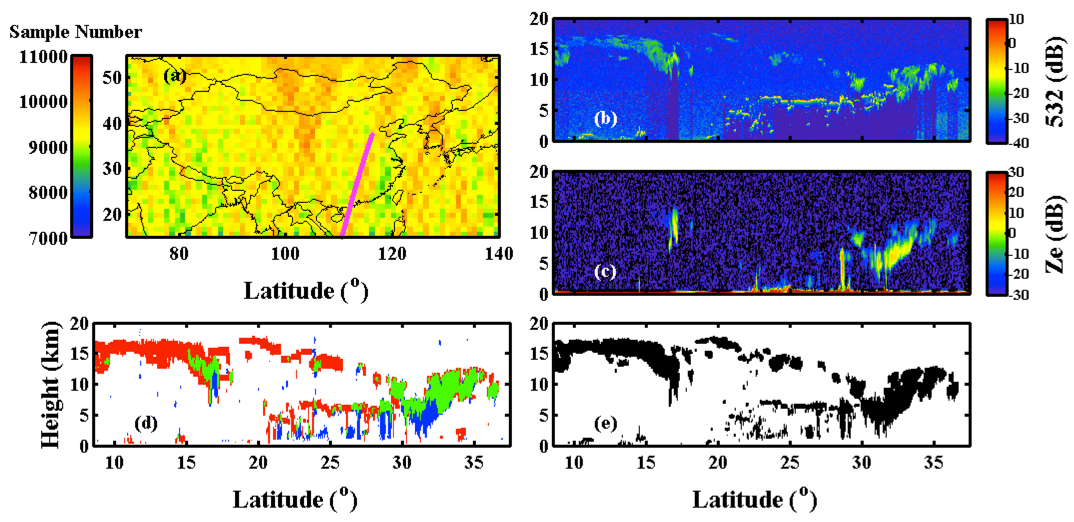
2. Datasets and Methodology

The latest version (R04) of the CloudSat 2B-CLDCLASS-LIDAR product [30] (Wang et al., 2012) between 2007–2010 is employed to study the cloud distributions and other macrophysical properties over East Asia. The sample number over the study region is shown in Figure 1a.
The 2B-CLDCLASS-LIDAR product combined measurements of the Cloud–Aerosol LIdar with Orthogonal Polarization (CALIOP) on CALIPSO and 94.05 GHz Cloud Profiling Radar (CPR) on CloudSat for cloud scenario classification. CALIOP is a near nadir-viewing two-wavelength lidar at 532 nm and 1064 nm, and linear polarization measurements at 532 nm [31]. Its vertical and horizontal resolutions are 30 m and 333 m below 8.2 km, and 60 m and 1000 m between 8.2–20.2 km, respectively. Due to its high vertical resolution, CALIOP is sensitive to most of the clouds and aerosols, and can detect their fine structure [24]. However, CALIOP is unable to penetrate optically thick clouds to detect anything beyond them due to strong attenuation at its short wavelength. CPR has a detection sensitivity of approximately −30 dBZ, with a vertical resolution of about 240 m between the surface and 30 km above ground level (AGL) and a horizontal footprint of 1.3 km cross-track and 1.7 km along-track. CPR is sensitive to large-sized particles such as ice and drizzle drops with relatively coarser resolution [32,33], and can penetrate optically thick clouds to detect multilayer cloud systems. However, its long wavelength limits its capability to detect water clouds with relatively small water droplets, or cold ice clouds with low concentrations of small ice crystals. Therefore, CALIOP and CPR measurements provide unique complementary capabilities for each other [32].
The 2B-CLDCLASS-LIDAR product firstly uses the radar cloud mask from CloudSat 2B-GEOPROF [33] and the CALOP cloud mask identified from the attenuated backscattering coefficient profile [34,35] as inputs to search for cloud clusters and generate cloud feature information, including cloud boundary height, temperature, thickness, fraction, precipitation, etc. CALIOP attenuated backscattering coefficients are averaged to the CPR horizontal resolution, but keep its native vertical resolutions for better cloud boundary and phase identifications. Temperature profiles from the European Center for Medium-Range Weather Forecast are interpolated to each CPR vertical bin, and are provided in the ECMWF-AUX product to determine cloud temperatures and assist in cloud classification [36]. Then, the CloudSat 2B-CLDCLASS-LIDAR product uses these cloud features, together with a fuzzy logical-based algorithm, to further classify clouds into different cloud types and determine cloud thermodynamic phases. Eight cloud types were classified, including cumulus (Cu), stratocumulus (Sc), stratus (St), altocumulus (Ac), altostratus (As), nimbostratus (Ns), cirrus (ci), and deep convective clouds (Dc). Furthermore, three cloud thermodynamic phases were determined: water, ice, and mixed phase.
The 2B-CLDCLASS-LIDAR product can provide more accurate detections of cloud boundaries and their vertical structures over the global scale than lidar-only or radar-only measurements. Figure 1 presents an example of A-Train satellite measurements and cloud detections from different products on 31 May 2008. Various cloud types and multilayer clouds can be observed from CALIOP total attenuated backscattering (TAB) at 532 nm (Figure 1b) and CPR radar reflectivity (Ze, Figure 1c). The lidar-only cloud mask (red and green patches) from the CALIOP level 2 5-km cloud layer product [37] and radar-only cloud mask (blue and green patches) from the CloudSat 2B-GEOPROF product [38] are shown in Figure 1d. It can be seen that CPR is not able to detect most of thin Ci and non-precipitating liquid clouds, while CALIOP is not able to penetrate liquid-topped clouds that occur within latitudes between 20.5–30.0 N to provide cloud information below the layer. With combined CPR and CALIOP measurements, a complete view of the cloud can be derived, which is shown as the cloud mask from 2B-CLDCLASS-LIDAR in Figure 1e.
Note that although the 2B-CLDCLASS-LIDAR is by far the most accurate satellite-based cloud product, it still has some limitations. For example, this product cannot detect some non-precipitation water clouds if there is optically thick cloud above, due to the detection limitations of radar and lidar measurements. Furthermore, the 2B-CLDCLASS-LIDAR keeps the CALIOP high vertical resolution measurements to derive the fine structure of the clouds, especially for optically thin clouds, which are transparent for Lidar. However, for optically thick clouds such as liquid, the identification of the cloud bottom mainly relies on CRP, which could result in an underestimation of cloud thicknesses due to its low sensitivity for small-size particles. Furthermore, the sparse temporal and space sampling of CPR and CALIOP measurements may also result in biases in our results. The non-convective clouds have small diurnal variations [39,40,41], while strong diurnal variations are seen for convective clouds. Due to its sun-synchronous orbit with only two overpasses at about 0130 and 1330 local time, A-Train satellites cannot capture the strongest or most frequent afternoon convective period [39]. However, the results from averaging both the day and the night A-train satellite measurements are close to the mean derived from The Tropical Rainfall Measuring Mission (TRMM) full-day samples [39]. Therefore, results with both day and night-time measurements were presented in this study. Although reliable observations are currently lacking, further investigations and evaluations of this product are still needed, and will be done in future study.

3. Results and Discussions

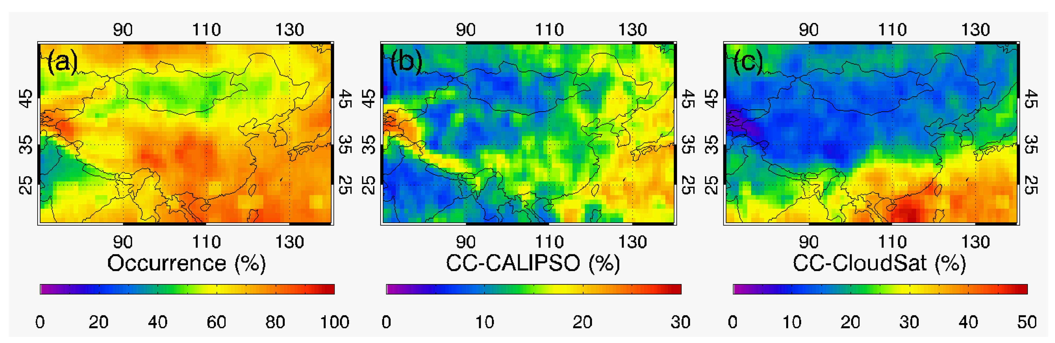
3.1. Cloud Occurrences

Cloud occurrence is defined as the ratio of a cloudy profile amount over the total measurement profile amount in a 1° (latitude) × 1° (longitude) box in this study. In a statistical point of view, cloud occurrence is equivalent to the commonly used cloud fraction in models. Cloud occurrence is a fundamental parameter through which clouds exert impacts on atmosphere radiation budgets. On average, cloud occurrence over East Asia is 66.3% with a standard deviation of 12.6%, compared with mean cloud occurrences of 52.5% from the CALIOP level 2 5-km cloud layer product and 44.7% from the CloudSat 2B-GEOPROF product.
The cloud occurrence distributions over East Asia from four years of the CloudSat 2B-CLDCLASS-LIDAR product are given in Figure 2a. From Figure 2a, cloud occurrences larger than 80% occur downstream of the Tibetan Plateau and over the East China Sea. Large cloud occurrences downstream of the Tibetan Plateau are consistent with Li and Gu [12]’s study, which showed that the dynamic and thermodynamic effects of the Tibetan Plateau provide favorable conditions for stratiform clouds. Figure 2b presents the differences of cloud occurrence frequencies between the CloudSat 2B-CLDCLASS-LIDAR product and the CALIOP Level 2 5-km cloud layer product. In general, cloud occurrences from the CloudSat 2B-CLDCLASS-LIDAR product are approximately 20% larger those that from the CALIOP Level 2 5-km cloud layer product along the south of Tibetan Plateau and over the South and East China Sea area. This is caused by the occurrence of large, deep, convective mid-level and low-level clouds over this region. Deep convective and mid-level clouds attenuate the CALIOP signal dramatically, which prevents CALIOP from detecting low-level clouds. Note that the performance of the CALIOP Level 2 5-km cloud layer product is similar to that of the CALIPSO-GOCCP reported in Yin et al. [7], which determines the cloud with a CALIOP scattering ratio at the resolution of the GCM [22]. Figure 2c shows the cloud occurrence differences between the CloudSat 2B-CLDCLASS-LIDAR product and the 2B-GEOPROF product. Differences larger than 30% occur over most of the southern area of East Asia, which is caused by large cirrus cloud occurrences that are out of the detection limit of the CPR over the region.
Figure 3 shows the zonally averaged vertical distribution of cloud occurrence over East Asia from the CloudSat 2B-CLDCLASS-LIDAR product and its differences from that of the CALIOP level 2 5-km cloud layer product and that of the CloudSat 2B-GEOPROF product. The height bin uses a CPR vertical resolution of 0.24 km, and the latitude bin size is 1°. From Figure 3a, we can see large cloud occurrences in altitudes between 10–18 km AGL at latitudes lower than 25 N, with maximum values greater than 30% at approximately 15 km AGL. There are also significant amounts of cloud below 2 km AGL at latitudes lower than 25 N. Within 25 N to 35 N, cloud occurrences decrease gradually from 30% near the surface to lower than 10% at about 11 km AGL. Within 45 N and 50 N, clouds mainly occur at altitudes between 4–10 km AGL, with an average occurrence of approximately 15%. At latitudes higher than 50 N, cloud occurrences decrease slightly, with heights below 11 km AGL. From Figure 3b, the CALIOP level 2 5-km cloud layer product significantly underestimates cloud occurrences below 11 km AGL at latitudes lower than 25 N, because deep convective clouds strongly attenuate CALIOP signals. At latitudes higher than 25 N, significant underestimations of cloud occurrences from the CALIOP level 2 5-km cloud layer product mainly occur at altitudes lower than 5 km AGL. Figure 3c shows that compared with the CloudSat 2B-CLDCLASS-LIDAR product, the 2B-GEOPROF product greatly underestimates high-level clouds at latitudes lower than 25 N and mid-altitude clouds at latitudes higher than 40 N. The 2B-GEOPROF product also slightly underestimates low-level non-precipitating clouds, as shown in Figure 3c.
CPR and CALIOP measurements also provide high-resolution vertically resolved detections of cloud structures and their seasonal variations. Figure 4 shows the seasonal variations and anomalies of zonally averaged vertical distributions of cloud occurrence over East Asia from the CloudSat 2B-CLDCLASS-LIDAR product. From the figure, we can see large seasonal variations of cloud occurrence at mid and high altitudes over latitudes lower than 25 N, with maximum values during June, July, and August (JJA) and minimum values during December, January, and February (DJF). This feature is directly caused by more and stronger convections during summer, and less and weaker convections during winter. For latitudes higher than 25 N, seasonal variations of cloud occurrence mainly occur at mid and low altitudes, with maximum values during March, April, and May (MAM) and minimum values during September, October, and November (SON). These signatures can be more clearly seen in the seasonal anomaly figures (as shown in the lower panel). Cloud occurrences at mid and high altitudes at latitudes lower than 25 N have seasonal variations as large as approximately 40%, while cloud occurrences at mid and low altitudes at latitudes higher than 25 N only have seasonal variations of less than 10%. Interestingly, clear seasonal variations of a narrow mid-altitude cloud band at altitudes between 8–12 km AGL at latitudes higher than 35 N can be seen in the seasonal anomaly figures. This narrow mid-altitude cloud band has maximum occurrences during MAM and JJA, and minimum occurrences during DJF. The seasonal variability of this mid-altitude cloud band may relate to the seasonal variation of the sub-tropic westerly, which plays a dominant role in transporting water vapor into northwest China [42,43,44,45]. The formation mechanism and season variation of this narrow mid-altitude cloud band will be further explored in future study.
Figure 5 shows the probability distribution functions (PDF) of cloud top and base heights, top temperature, and their seasonal variations over East Asia. Johnson et al. [46] showed trimodal cloud distributions at approximately 2 km, 5 km, and 15 km over the tropics. From Figure 5a, cloud occurrence over East Asia has similar low-altitude (1.5 km) and high-altitude (15 km) peaks all of the time, and a very small peak around 5–6 km in JJA and MAM. Unlike over the tropics, there is another high-altitude peak at 10 km over East Asia all of the time. The two high-altitude peaks at 15 km and 10 km result from the high-altitude clouds (mainly cirrus), which is consistent with the cloud vertical distributions shown in Figure 4. The cirrus has quite different behaviors in cloud-top height over the sub-tropic and mid-latitude regions (~10–11 km), and over the tropics (~15 km) [43]. The peak at 10 km has a relatively smaller seasonal variation than the 15-km peak, which may be the result of different formations of Ci over different regions. Over mid-latitudes, the cirrus tends to form from cloud top ice nucleating zones, where ice supersaturations are relatively high, from the homogeneous nucleation of haze particles [47]. However, over the tropics, cirrus is mainly formed by strong updrafts in deep convective clouds, bringing water vapor and cloud nuclei from the near surface upward until it is blocked by the top of the tropopause (~15 km). Therefore, the 15-km peak is largest in JJA and smallest in DJF, corresponding to the deep convection activates in these two seasons. As for cloud base height, PDFs decrease quickly until 2 km AGL, and then start to decrease slowly with altitude. Similar to Figure 5a, JJA has the smallest PDFs at low altitudes and largest values at high altitudes, and vice versa for DJF. The PDFs of cloud top temperature have large values and small seasonal variations within the temperature range between −30 °C and 10 °C. At low temperatures, there are two distinct local PDF peaks at approximately −60 °C and −85 °C, corresponding to the 10-km and 15-km peaks in cloud-top height, respectively. The different cloud top temperature indicates different ice growth habits and rates of Ci between the tropics and mid-latitudes.

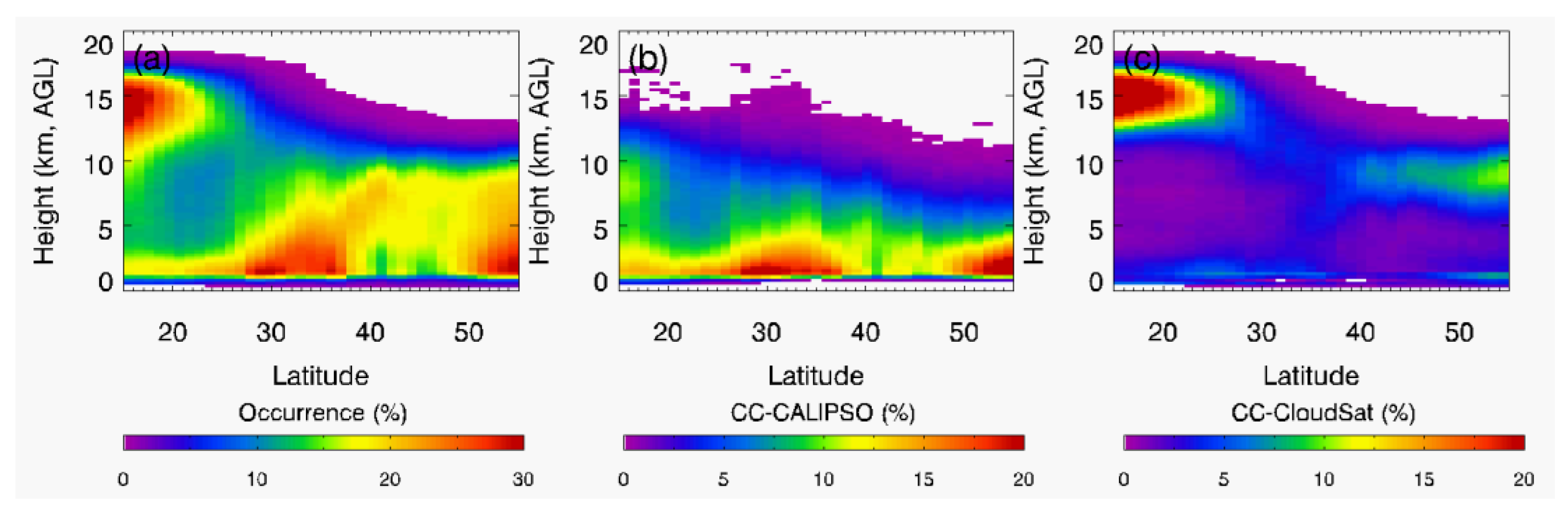
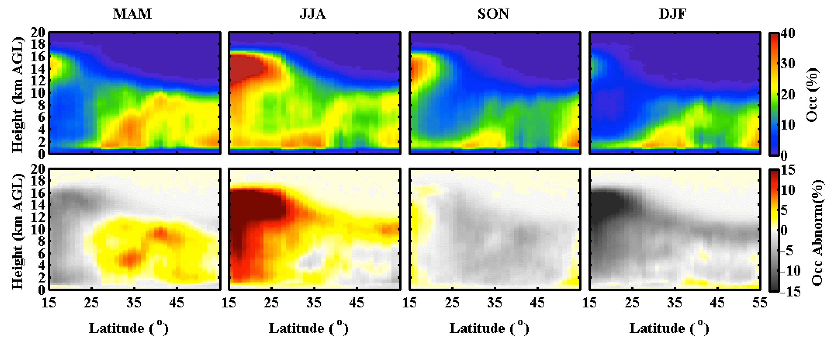
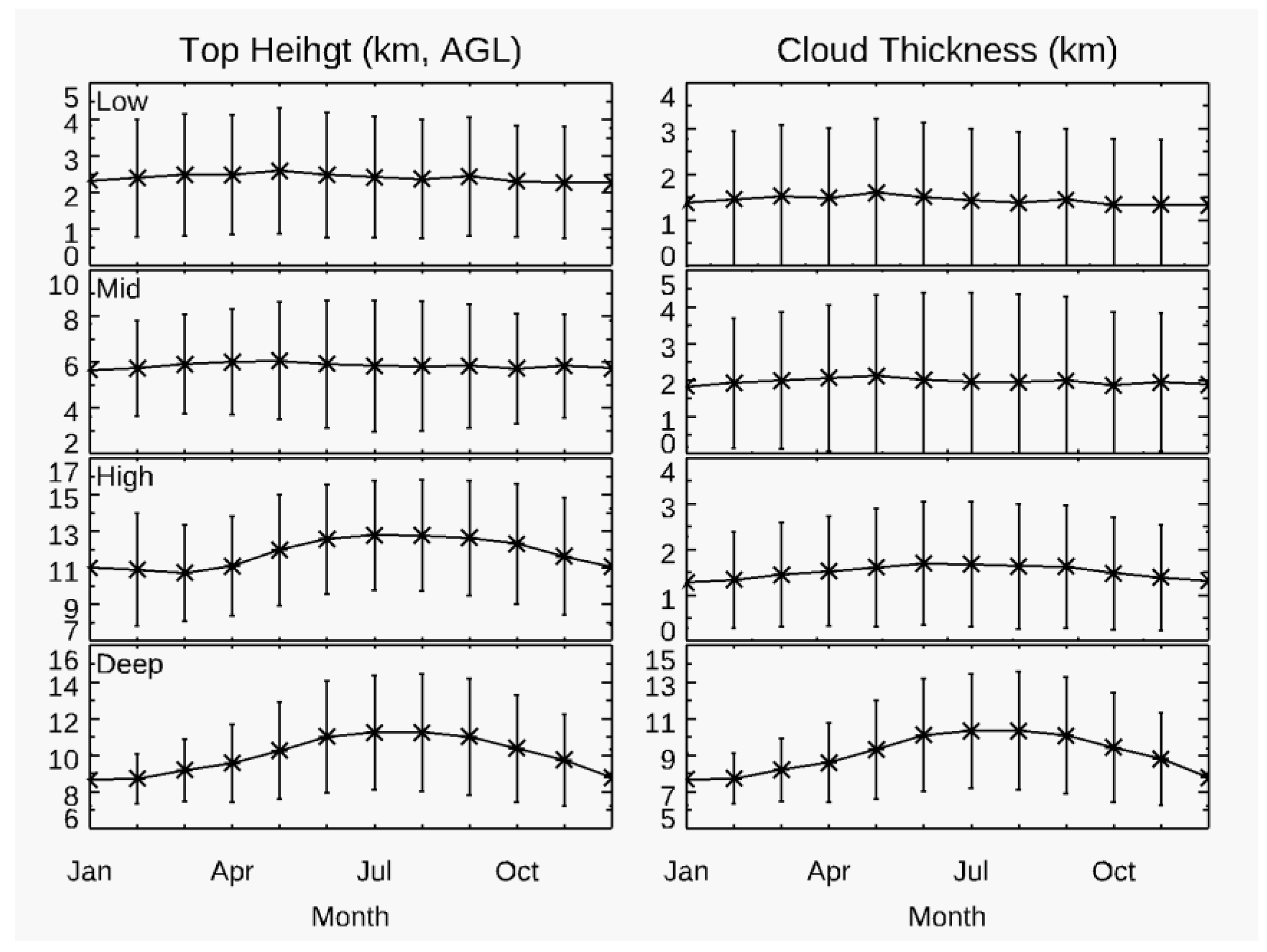
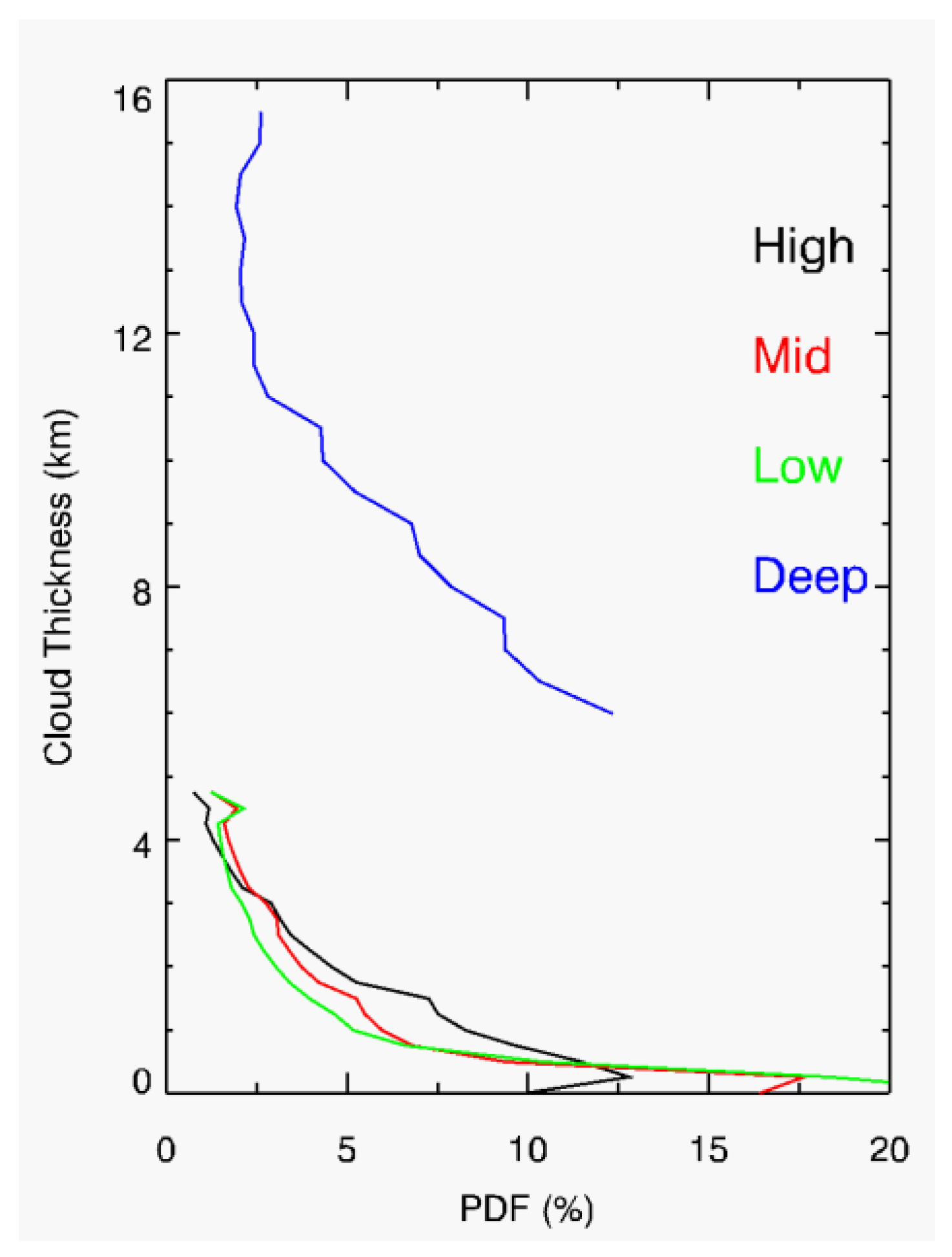
3.2. Cloud Distributions at Different Altitude Levels

To better understand the dynamic and thermodynamic environments associated with cloud distributions, the clouds are classified into high-level (cloud base ≥ 6 km AGL), mid-level (6 km > cloud base ≥ 2 km AGL), and low-level (cloud base < 2 km AGL and cloud thickness < 6 km) clouds and vertically extended deep cloud systems (cloud base < 2 km AGL and cloud thickness ≥ 6 km), following Adhikari et al. [48]’s criteria. The adopted thresholds of cloud base height are commonly used in the literature and meteorological departments (such as the Met Office and National Weather Service). The threshold of 6-km cloud thickness to distinguish low clouds from deep cloud systems is also chosen based on the consideration that the low clouds are mainly stratiform clouds and stratocumulus clouds, whose cloud thicknesses are mostly smaller than 6. Figure 6 shows distributions of cloud occurrence for low-level, mid-level, high-level, and deep clouds over East Asia from four years of the CloudSat 2B-CLDCLASS-LIDAR product. From the figure, low-level clouds mainly occur in the southwest of China, with occurrences larger than 60%, and over the East and South China Sea, with occurrences of approximately 50%. Mid-level clouds are widely distributed over East Asia, and have occurrences of approximately 30%, with larger occurrences of approximately 40% in the middle of China. High-level clouds are concentrated within southern East Asia, with occurrences generally larger than 70%. Deep clouds are mainly located at the Bay of Bengal and the East China Sea, with occurrences of approximately 10%. Please note that the color bar magnitude in Figure 6d is smaller than that for the other three.
Seasonal variations and anomalies of cloud occurrence distributions for low-level, mid-level, high-level, and deep clouds are presented in Figure 7 and Figure 8, respectively. From Figure 7 (first panel), the largest occurrences of low-level clouds are in the southwest of China during JJA, with occurrences larger than 70%, and over the East and South China Sea during DJF, with occurrences larger than 60%. From Figure 8 (first panel), these two regions also have large seasonal variations of low-level cloud occurrences, of up to 40%. As for mid-level clouds, the largest cloud occurrences of 50% occur over the northwest of China during MAM. From Figure 8 (second row), the northwest of China also has strong seasonal variations of mid-level cloud occurrences, with positive anomalies during MAM and negative anomalies during SON. In addition, southwestern East Asia has strong seasonal variations of mid-level cloud occurrences, with positive anomalies during JJA and negative anomalies during DJF. For high-level clouds, as shown in Figure 7 (third row), cloud occurrences during JJA not only have higher magnitudes of 90%, this also extends to higher latitudes. The signatures can be clearly seen in Figure 8 (third panel), with large positive anomalies during JJA and negative anomalies during DJF. From Figure 8 (third panel), there is another band of high-level clouds over northwestern East Asia that has strong seasonal variations with positive anomalies during MAM and negative anomalies during JJA and SON. From Figure 7 (fourth row), similar to high-level cloud distributions, deep clouds have their largest occurrences over southern East Asia during JJA, and their smallest occurrences during DJF. This region also has the strongest seasonal variations, with positive anomalies during JJA and negative anomalies during DJF.

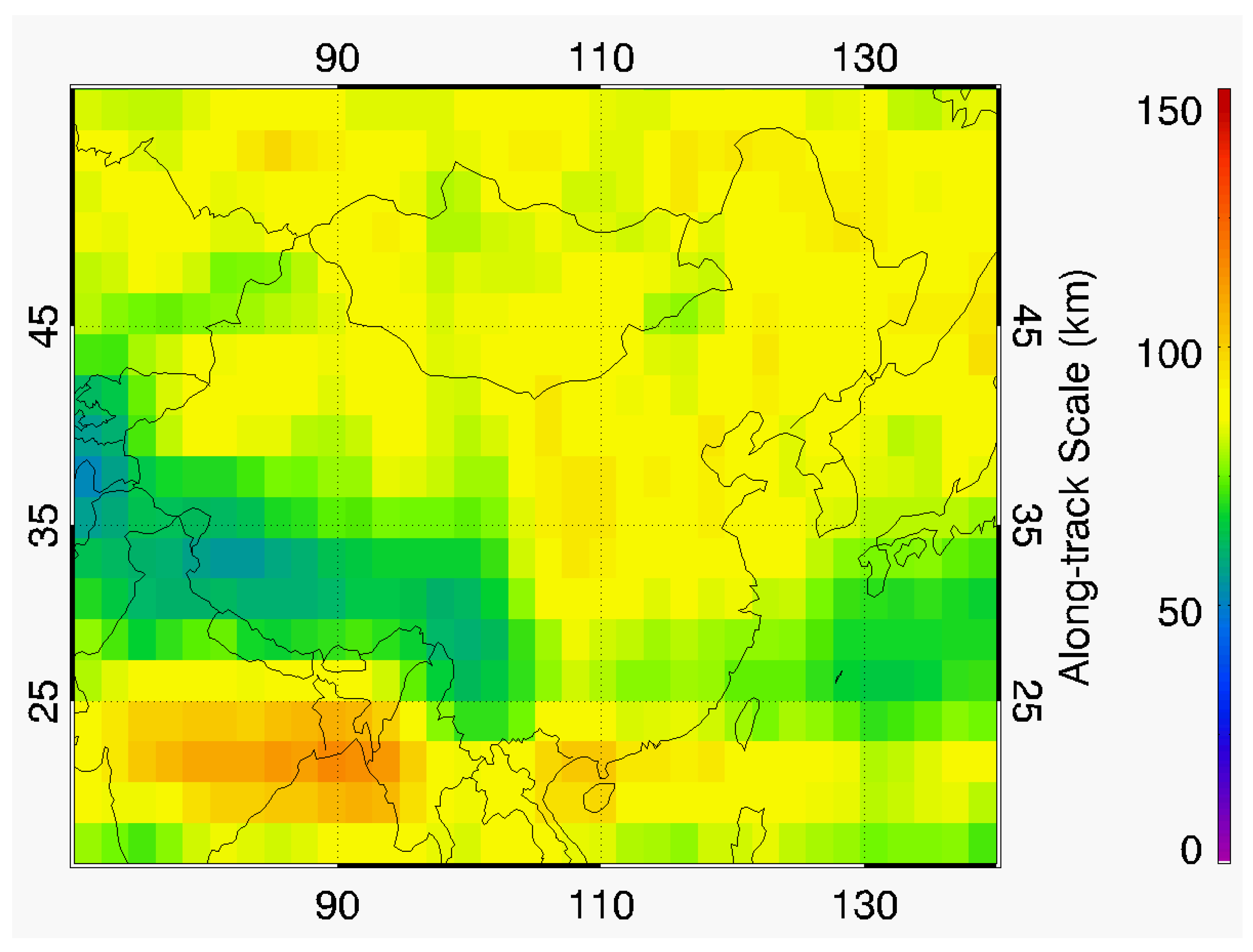
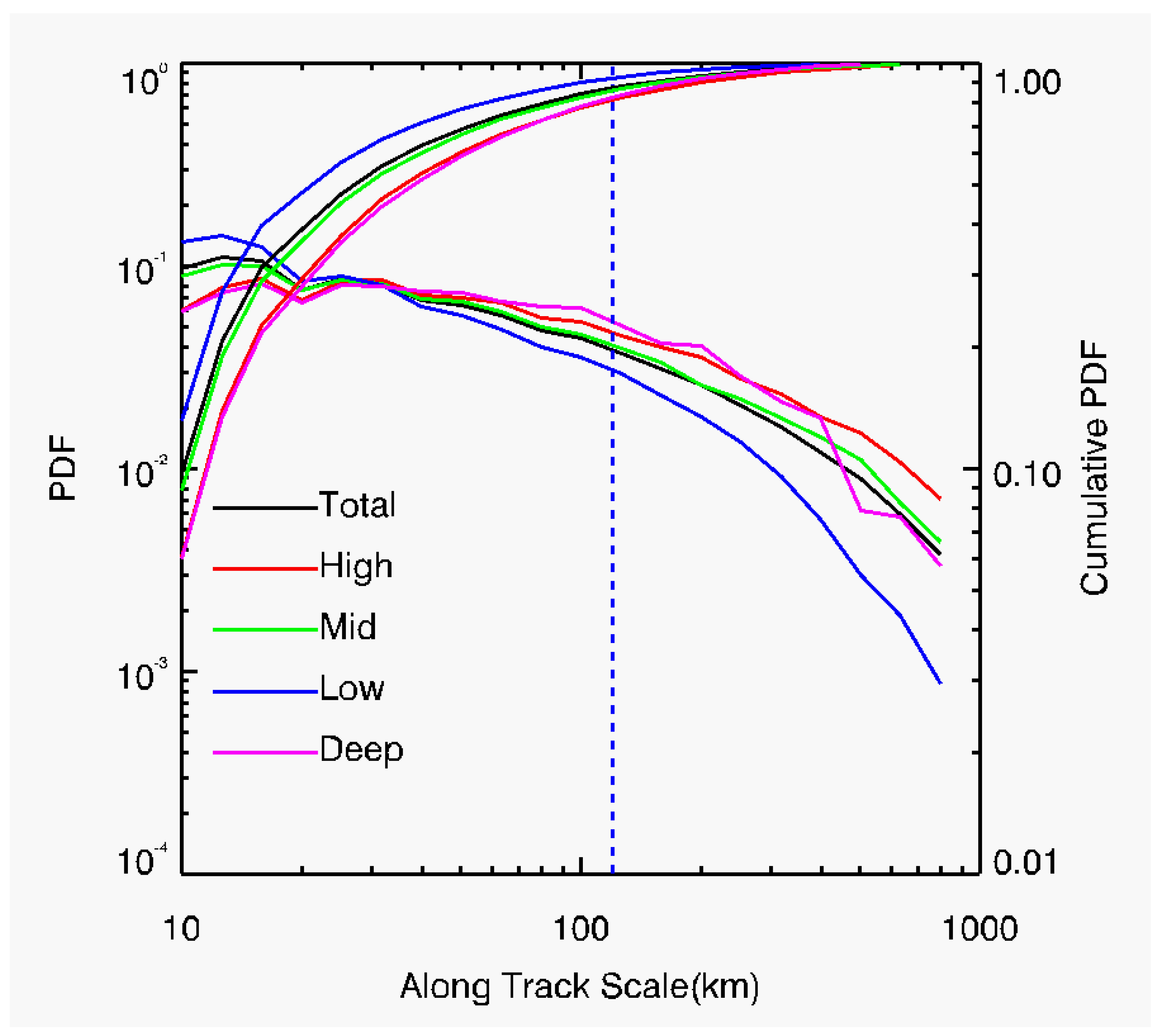
3.3. Discussions about Cloud Vertical and Horizontal Scales

The radiative impacts of clouds are directly affected by their horizontal coverage and vertical extensions. Collocated CPR and CALIOP measurements provide reliable detections of cloud systems and their along-track horizontal scales.
Figure 9 shows the time series of monthly averaged cloud-top height and cloud thickness for low-level, mid-level, high-level, and deep clouds. From Figure 9, low-level and mid-level cloud-top heights and thicknesses have little monthly variations. For high-level clouds, cloud-top height is about 2 km larger during JJA, but cloud thicknesses have little monthly variations. For deep clouds, both cloud-top height and thickness are about 2 km larger during JJA.
To take a closer look at cloud vertical distributions, Figure 10 shows the PDFs of cloud thickness for low-level, mid-level, high-level, and deep clouds. Their mean cloud-top heights (km AGL) and cloud thicknesses are given in Table 1. From the figure, the PDFs of low-level, mid-level, and high-level cloud thickness have a peak value that is smaller than 0.5 km, and then decrease gradually with cloud thickness, with the mean thicknesses smaller than ~2 km in Table 1. This indicates that models with vertical resolutions lower than 0.5 km have difficulties resolving those clouds. The PDFs of deep cloud thickness generally decrease with cloud thickness. It should be noted that due to the strong attenuation of the lidar signal by liquid layers and the low sensitivity of the CPR and attenuation of the radar signal by strong convective clouds, the CloudSat 2B-CLDCLASS-LIDAR product may underestimate cloud thicknesses for non-precipitating liquid clouds and deep convective clouds.
For cloud horizontal scales, a cloud system is first identified using the CloudSat 2B-CLDCLASS-LIDAR product following Zhang et al. [49]’s method. The horizontal scale of a cloud system along the CALIPSO/CloudSat track is then determined by calculating the continuous profiles (N) of a detected cloud system. Considering the 1.7-km along-track resolution of CPR measurements, the along-track scale (L in km) of a cloud system is L = N × 1.7. The distribution of cloud along-track horizontal scales over East Asia is shown in Figure 11. The averaged cloud along-track horizontal scale over East Asia is 82.0 km, with a standard deviation of 142.0 km. From the figure, the largest cloud along-track horizontal scales are located in southwestern East Asia with values larger than 120 km, while the smallest cloud along-track horizontal scales are at the middle of western East Asia, with values smaller than 50 km.
Figure 12 shows the PDFs and cumulative PDFs of along-track horizontal scales for total, low-level, mid-level, high-level, and deep clouds. Assuming a typical grid resolution of 1° in climate models, which is about 110 km (blue dashed line in Figure 12), approximately 81.2% of the clouds over East Asia have horizontal scales smaller than the model grid resolution on a global average, and cannot be resolved by climate models. From Figure 12, the PDFs decrease dramatically as the along-track horizontal scale increases for all of the cloud types. The mean along-track horizontal scales for low-level, mid-level, high-level, and deep clouds are 56 km, 88 km, 110 km, and 99 km, respectively. Comparing the along-track horizontal scale for different cloud types, low-level clouds have the smallest along-track horizontal scales, while high-level clouds have the largest along-track horizontal scales. Note that the statistical behaviors of along-track horizontal scale for different cloud types over the global are similar to those presented here.

4. Summary and Conclusions

In this study, four years (2007–2010) of CloudSat 2B-CLDCLASS-LIDAR product are analyzed to study cloud occurrences, vertical distributions, and along-track horizontal scales over East Asia. The CloudSat 2B-CLDCLASS-LIDAR product uses combined CPR and CALIOP measurements for cloud scenario classification, and provides by far the most accurate detections of cloud boundaries and their vertical structures on a global scale.
The mean occurrence frequency over East Asia derived from the CloudSat 2B-CLDCLASS-LIDAR product is 66.3% with a standard deviation of 12.6%, which is approximately 13.8% and 21.6% higher than that from the CALIOP level 2 5-km cloud layer product and the CloudSat 2B-GEOPROF product, respectively. These differences are even larger than the model-observation differences, as is pointed out in the introduction section, suggesting the importance of using more reliable cloud datasets for model validations. Significant differences in cloud occurrence between that of the CloudSat 2B-CLDCLASS-LIDAR product and that of the CALIOP Level 2 5-km cloud layer product occur along the south of the Tibetan Plateau and over the South and East China Sea area, while significant differences between that of the CloudSat 2B-CLDCLASS-LIDAR product and that of the 2B-GEOPROF product occur over most of the southern East Asia area. For vertical distributions, clouds occur frequently at high and low altitudes, with significant seasonal variations at latitudes lower than 25 N, and at mid and low altitudes, with less seasonal variations at latitudes higher than 25 N. Cloud-top heights over East Asia have three local peaks at approximately 1.5 km AGL corresponding to the low clouds, and 10 km and 15 km AGL corresponding to the high clouds over mid-latitude regions and the near-tropic regions, respectively.
To better understand cloud dynamic and thermodynamic environments, clouds are also classified into low-level clouds, mid-level clouds, high-level clouds, and vertically extended deep cloud systems. Except for over the East and South China Sea, low-level clouds mainly occur in the southwest of China around the Tibetan Plateau, as a result of the topography effect of the Tibetan Plateau on the circulation and thus the transport of water vapor. Mid-level clouds are widely distributed over East Asia, with larger occurrences in the middle of China, forming a mid-altitude cloud band related to the water vapor that is transported by the sub-tropic westerly. High-level clouds are concentrated within southern East Asia, and mostly occur in JJA, due to the deep convection and strong water vapor transport by the updraft. Deep clouds are mainly located over the Bay of Bengal and East China Sea. Significant seasonal variations for low-level clouds, mid-level clouds, high-level clouds, and deep clouds are found in different regions, which are related to different cloud formation mechanisms. Low-level and mid-level cloud-top heights and thicknesses have little monthly variations. For high-level clouds, cloud-top heights are about 2 km larger during JJA, but cloud thicknesses have little monthly variations. For deep clouds, both cloud-top height and thickness are about 2 km larger during JJA.
The vertical and horizontal scales of the clouds were analyzed in detail. Significant fractions of low-level cloud, mid-level cloud, and high-level cloud have thicknesses smaller than 1 km, which indicates that models with vertical resolutions lower than 0.5 km have difficulties reliably resolving those clouds. The averaged cloud along-track horizontal scale over East Asia is 82.0 km, with a standard deviation of 142.0 km. The PDFs of cloud along-track horizontal scales suggest that approximately 81.2% of the clouds over East Asia cannot be resolved by climate models with a grid resolution of 1°. Mean along-track horizontal scales for low-level clouds, mid-level clouds, high-level clouds, and deep clouds are 56 km, 88 km, 110 km, and 99 km, respectively. Low-level clouds have the smallest along-track horizontal scales, while high-level clouds have the largest along-track horizontal scales.
This study provides a unique and reliable dataset of cloud occurrences and morphology characteristics over East Asia. The dataset can be used to improve cloud parameterizations in climate models and validate model simulations of clouds over East Asia. Further analyses of cloud microphysical properties such as droplet effective radius, particle size, and water content retrieved from combined CloudSat radar and CALIPSO lidar measurements over East Asia are currently being conducted in our group.

Author Contributions

X.L. and W.Z. conceived and designed the study; X.Z. and W.Z. analyzed the data; F.W. downloaded the data; Y.D. contributed analysis tools; X.L. and X.Z. drafted the manuscript. D.Z. edited and critically revised the manuscript.

Funding

This research was funded by National Key Basic Research Program of China (2017YFC0209801) and Nature Science Research Project of Anhui province (1708085MD95).

Acknowledgments

CloudSat data are available at the CloudSat Data Processing Center (http://www.cloudsat.cira.colostate.edu). CALIOP data are available online at the NASA Langley Atmospheric Sciences Data Center website (https://eosweb.larc.nasa.gov/order-data). Many thanks go to the CALIPSO/CloudSat data group. The authors acknowledge the editors’ and referees’ efforts in improving the manuscript.

Conflicts of Interest

The authors declare no conflict of interest.

References

  1. Wielicki, B.A.; Barkstrom, B.R.; Harrison, E.F.; Lee, R.B., III; Louis Smith, G.; Cooper, J.E. Clouds and the Earth’s Radiant Energy System (CERES): An earth observing system experiment. Bull. Am. Meteorol. Soc. 1996, 77, 853–868. [Google Scholar] [CrossRef]
  2. Sassen, K.; Wang, Z. Classifying clouds around the globe with the CloudSat radar: 1-Year of results. Geophys. Res. Lett. 2008, 35. [Google Scholar] [CrossRef]
  3. Chen, T.; Rossow, W.; Zhang, Y. Radiative effects of cloud-type variations. J. Clim. 2000, 13, 264–286. [Google Scholar] [CrossRef]
  4. Stocker, T.F.; Qin, D.; Plattner, G.-K.; Tignor, M.; Allen, S.K.; Boschung, J.; Nauels, A.; Xia, Y.; Bex, V.; Midgley, P.M. (Eds.) Climate Change 2013: The Physical Science Basis. Contribution of Working Group I to the Fifth Assessment Report of the Intergovernmental Panel on Climate Change; Cambridge University Press: Cambridge, UK; New York, NY, USA, 2013; p. 1535. [Google Scholar]
  5. Zhang, M.H.; Lin, W.Y.; Klein, S.A.; Bacmeister, J.T.; Bony, S.; Cederwall, R.T.; Genio, A.D.; Del Hack, J.J.; Loeb, N.G.; Lohmann, U.; et al. Comparing clouds and their seasonal variations in 10 atmospheric general circulation models with satellite measurements. J. Geophys. Res. 2005, 110. [Google Scholar] [CrossRef]
  6. Zhang, D.; Wang, Z.; Liu, D. A global view of midlevel liquid-layer topped stratiform cloud distribution and phase partition from CALIPSO and CloudSat measurements. J. Geophys. Res. 2010, 115. [Google Scholar] [CrossRef]
  7. Yin, J.; Wang, D.; Xu, H.; Zhai, G. An investigation into the three-dimensional cloud structure over East Asia from the CALIPSO-GOCCP Data. Sci. China Earth Sci. 2015, 58, 2236–2248. [Google Scholar] [CrossRef]
  8. Fan, J.; Leung, L.R.; Li, Z.; Morrison, H.; Chen, H.; Zhou, Y.; Qian, Y.; Wang, Y. Aerosol impacts on clouds and precipitation in eastern China: Results from bin and bulk microphysics. J. Geophys. Res. 2012, 117. [Google Scholar] [CrossRef]
  9. Liu, J.; Li, Z.; Zheng, Y.; Chiu, J.C.; Zhao, F.; Cadeddu, M.; Weng, F.; Cribb, M. Cloud optical and microphysical properties derived from ground-based and satellite sensors over a site in the Yangtze Delta region. J. Geophys. Res. Atmos. 2013, 118, 9141–9152. [Google Scholar] [CrossRef]
  10. Yan, Y.; Liu, Y.; Lu, J. Cloud vertical structure, precipitation, and cloud radiative effects over Tibetan Plateau and its neighboring regions. J. Geophys. Res. Atmos. 2016, 121, 5864–5877. [Google Scholar] [CrossRef]
  11. Yu, R.; Wang, B.; Zhou, T. Climate Effects of the Deep Continental Stratus Clouds Generated by the Tibetan Plateau. J. Clim. 2004, 17, 2702–2713. [Google Scholar] [CrossRef]
  12. Li, Y.; Gu, H. Relationship between middle stratiform clouds and large scale circulation over eastern China. Geophys. Res. Lett. 2006, 33. [Google Scholar] [CrossRef]
  13. Kang, S.; Xu, Y.; You, Q.; Flügel, W.A.; Pepin, N.; Yao, T. Review of climate and cryospheric change in the Tibetan Plateau. Environ. Res. Lett. 2010, 5, 015101. [Google Scholar] [CrossRef] [Green Version]
  14. Lau, W.K.-M.; Kim, M.-K.; Kim, K.-M.; Lee, W.-S. Enhanced surface warming and accelerated snow melt in the Himalayas and Tibetan Plateau induced by absorbing aerosols. Environ. Res. Lett. 2010, 5, 025204. [Google Scholar] [CrossRef]
  15. Duan, A.; Xiao, Z. Does the climate warming hiatus exist over the Tibetan Plateau? Sci. Rep. 2015, 5, 13711. [Google Scholar] [CrossRef] [PubMed]
  16. Ding, Y.; Chan, J.C. The East Asian summer monsoon: An overview. Meteorol. Atmos. Phys. 2005, 89, 117–142. [Google Scholar]
  17. Johnson, R.H.; Houze, R.A. Precipitating Cloud Systems of the Asian Monsoon, Monsoon Meteorology; Chang, C.-P., Krishnamurti, T.N., Eds.; Oxford University Press: New York, NY, USA, 1987. [Google Scholar]
  18. Berry, E.; Mace, G.G. Cloud properties and radiative effects of the Asian summer monsoon derived from A-Train data. J. Geophys. Res. Atmos. 2014, 119, 9492–9508. [Google Scholar] [CrossRef]
  19. Li, J.; Waliser, D.; Stephens, G.; Lee, S. Characterizing and Understanding Cloud Ice and Radiation Budget Biases in Global Climate Models and Reanalysis. Meteorol. Monogr. 2016, 56, 13.1–13.20. [Google Scholar] [CrossRef]
  20. Li, Y.; Yu, R.C.; Xu, Y.P.; Zhang, X.H. Spatial distribution and seasonal variation of cloud over China based on ISCCP data and surface observations. J. Meteorol. Soc. Jpn. 2004, 82, 761–773. [Google Scholar] [CrossRef]
  21. Yin, J.; Wang, D.; Zhai, G.; Wang, Z. Observational characteristics of cloud vertical profiles over the continent of East Asia from the CloudSat data. Acta Meteorol. Sin. 2013, 27, 26–39. [Google Scholar] [CrossRef]
  22. Chepfer, H.; Bony, S.; Winker, D.; Cesana, G.; Dufresne, J.L.; Minnis, P.; Stubenrauch, C.J.; Zeng, S. The GCM-Oriented CALIPSO Cloud Product (CALIPSO-GOCCP). J. Geophys. Res. 2010, 115. [Google Scholar] [CrossRef]
  23. Bühl, J.; Seifert, P.; Myagkov, A.; Ansmann, A. Measuring ice- and liquid-water properties in mixed-phase cloud layers at the Leipzig Cloudnet station. Atmos. Chem. Phys. 2016, 16, 10609–10620. [Google Scholar] [CrossRef]
  24. Winker, D.M.; Pelon, J.; Coakley, J.A., Jr.; Ackerman, S.A.; Charlson, R.J.; Colarco, P.R.; Flamant, P.; Fu, Q.; Hoff, R.M.; Kittaka, C. The CALIPSO mission: A global 3D view of aerosols and clouds. Bull. Am. Meteorol. Soc. 2010, 91, 1211–1230. [Google Scholar] [CrossRef]
  25. Su, H.; Jiang, J.H.; Zhai, C.; Perun, V.S.; Shen, J.T.; Genio, A.D.; Nazarenko, L.S.; Donner, L.J.; Horowitz, L.; Seman, C.; et al. Diagnosis of regime-dependent cloud simulation errors in CMIP5 models using “A-Train” satellite observations and reanalysis data. J. Geophys. Res. Atmos. 2013, 118, 2762–2780. [Google Scholar] [CrossRef]
  26. Cesana, G.; Waliser, D.E. Characterizing and understanding sys-tematic biases in the vertical structure of clouds in CMIP5/CFMIP2 models. Geophys. Res. Lett. 2016, 43, 10538–10546. [Google Scholar] [CrossRef]
  27. Myers, T.A.; Norris, J.R. On the Relationships between Subtropical Clouds and Meteorology in Observations and CMIP3 and CMIP5 Models. J. Clim. 2015, 28, 2945–2967. [Google Scholar] [CrossRef]
  28. Luo, Y.; Zhang, R.; Wang, H. Comparing Occurrences and Vertical Structures of Hydrometeors between Eastern China and the Indian Monsoon Region Using CloudSat/CALIPSO Data. J. Clim. 2009, 22, 1052–1064. [Google Scholar] [CrossRef]
  29. Mace, G.G.; Zhang, Q.; Vaughan, M.; Marchand, R.; Stephens, G.; Trepte, C.; Winker, D. A description of hydrometeor layer occurrence statistics derived from the first year of merged Cloudsat and CALIPSO data. J. Geophys. Res. 2009, 114. [Google Scholar] [CrossRef]
  30. Wang, Z.; Vane, D.; Stephens, G.; Reinke, D. Level 2 Combined Radar and Lidar Cloud Scenario Classification Product Process Description and Interface Control Document; Jet Propulsion Laboratory; California Institute of Technology: Pasadena, CA, USA, 2012; 22p, Available online: http://www.cloudsat.cira.colostate.edu/sites/default/files/products/files/2B-CLDCLASS-LIDAR_PDICD.P_R04.20120522.pdf (accessed on 22 May 2012).
  31. Winker, D.M.; Pelon, J.R.; McCormick, M.P. The CALIPSO mission: Spaceborne Lidar for observation of aerosols and clouds. In Lidar Remote Sensing for Industry and Environment Monitoring III, Proceedings of the 3rd International Asia-Pacific Environmental Remote Sensing Remote Sensing of the Atmosphere, Ocean, Environment, and Space, Hangzhou, China, 23–27 October 2002; Singh, U.N., Itabe, T., Lui, Z., Eds.; International Society for Optical Engineering: Washington, DC, USA, 2003; Volume 4893, pp. 1–11. [Google Scholar]
  32. Stephens, G.L.; Boain, R.J.; Mace, G.G.; Sassen, K.; Wang, Z.; Illingworth, A.J.; O’Connor, E.J.; Rossow, W.J.; Durden, S.L.; Miller, S.D.; et al. The CloudSat mission and the A-Train. Bull. Am. Meteorol. Soc. 2002, 83, 1771–1790. [Google Scholar] [CrossRef]
  33. Stephens, G.L.; Tanelli, S.; Im, E.; Durden, S.; Rokey, M.; Reinke, D.; Partain, P.; Mace, G.G.; Austin, R.; L’Ecuyer, T.; et al. CloudSat mission: Performance and early science after the first year of operation. J. Geophys. Res. 2008, 113. [Google Scholar] [CrossRef]
  34. Mace, G.G.; Marchand, R.; Zhang, Q.; Stephens, G. Global hydrometeor occurrence as observed by CloudSat: Initial observations from summer 2006. Geophys. Res. Lett. 2007, 34. [Google Scholar] [CrossRef]
  35. Wang, Z.; Sassen, K. Cloud type and macrophysical property retrieval using multiple remote sensors. J. Appl. Meteorol. 2001, 40, 1665–1682. [Google Scholar] [CrossRef]
  36. Partain, P. Cloudsat ECMWF-AUX Auxiliary Data Process Description and Interface Control Document; Cooperative Institute for Research in the Atmosphere, Colorado State University: Fort Collins, CO, USA, 2007; p. 80523. [Google Scholar]
  37. Liu, Z.; Vaughan, M.; Winker, D.; Kittaka, C.; Getzewich, B.; Kuehn, R.; Omar, A.; Powell, K.; Trepte, C.; Hostetler, C. The CALIPSO Lidar Cloud and Aerosol Discrimination: Version 2 Algorithm and Initial Assessment of Performance. J. Atmos. Ocean. Technol. 2009, 26, 1198–1213. [Google Scholar] [CrossRef]
  38. Marchand, R.; Mace, G.G.; Ackerman, T.; Stephens, G. Hydrometeor Detection Using CloudSat—An Earth-Orbiting 94-GHz Cloud Radar. J. Atmos. Ocean. Technol. 2008, 25, 519–533. [Google Scholar] [CrossRef]
  39. Liu, C.; Zipser, E.J.; Mace, G.; Benson, S. Implications of the differences between daytime and nighttime CloudSat observations over the tropics. J. Geophys. Res. 2008, 113. [Google Scholar] [CrossRef]
  40. Bouniol, D.; Couvreux, F.; Kamsu-Tamo, P.-H.; Leplay, M.; Guichard, F.; Favot, F.; O’Connor, E.J. Diurnal and Seasonal Cycles of Cloud Occurrences, Types, and Radiative Impact over West Africa. J. Appl. Meteorol. Clim. 2012, 51, 534–553. [Google Scholar] [CrossRef]
  41. Zuidema, P.; Mapes, B. Cloud Vertical Structure Observed from Space and Ship over the Bay of Bengal and the Eastern Tropical Pacific. J. Meteorol. Soc. Jpn. 2008, 86, 205–218. [Google Scholar] [CrossRef]
  42. Li, W.L.; Wang, K.L.; Fu, S.M.; Jiang, H. The interrelationship between regional westerly index and the water vapor budget in northwest China. J. Glaciol. Geocryol. 2008, 30, 34–38. (In Chinese) [Google Scholar]
  43. Chen, T.; Guo, J.; Li, Z.; Zhao, C.; Liu, H.; Cribb, M.; Wang, F.; He, J. A CloudSat Perspective on the Cloud Climatology and Its Association with Aerosol Perturbations in the Vertical over Eastern China. J. Atmos. Sci. 2016, 73, 3599–3616. [Google Scholar] [CrossRef]
  44. Ren, G.Y.; Yuan, Y.J.; Liu, Y.J.; Ren, Y.Y.; Wang, T.; Ren, X.Y. Changes in precipitation over northwest China. Arid Zone Res. 2016, 33, 1–19. (In Chinese) [Google Scholar] [CrossRef]
  45. Peng, D.; Zhou, T. Why was the arid and semiarid northwest China getting wetter in the recent decades? J. Geophys. Res. Atmos. 2017, 122, 9060–9075. [Google Scholar] [CrossRef]
  46. Johnson, R.H.; Rickenbach, T.M.; Rutledge, S.A.; Ciesielski, P.E.; Schubert, W.H. Trimodal Characteristics of Tropical Convection. J. Clim. 1999, 12, 2397–2418. [Google Scholar] [CrossRef]
  47. Sassen, K.; Wang, Z.; Liu, D. Global distribution of cirrus clouds from CloudSat/Cloud-Aerosol Lidar and Infrared Pathfinder Satellite Observations (CALIPSO) measurements. J. Geophys. Res. 2008, 113. [Google Scholar] [CrossRef]
  48. Adhikari, L.; Wang, Z.; Deng, M. Seasonal variations of Antarctic clouds observed by CloudSat and CALIPSO satellites. J. Geophys. Res. 2012, 117. [Google Scholar] [CrossRef]
  49. Zhang, D.; Luo, T.; Liu, D.; Wang, Z. Spatial scales of altocumulus clouds observed with collocated CALIPSO and CloudSat measurements. Atmos. Res. 2014, 149, 58–69. [Google Scholar] [CrossRef]
Figure 1. An example of A-Train satellite measurements and cloud detections on 31 May 2008. (a) Sample number of the four-year A-Train satellite measurements over the study region, overlaid with the magenta line indicating the location of the case; (b) Cloud–Aerosol LIdar with Orthogonal Polarization (CALIOP) total attenuated backscattering (TAB) at 532 nm; (c) Cloud Profiling Radar (CPR) reflectivity (Ze); (d) clouds detected with CloudSat 2B-GEOPROF (blue) and CALIOP level 2 5-km cloud layer product (red), green regions represent clouds seen from both products; and (e) clouds detected with CloudSat 2B-CLDCLASS-LIDAR product.
Atmosphere 09 00168 g001
Figure 2. (a) Cloud occurrence frequencies from four-year (2007–2010) CloudSat 2B-CLDCLASS-LIDAR product; (b) differences of cloud occurrence frequencies between the CloudSat 2B-CLDCLASS-LIDAR product and the CALIOP Level 2 5-km cloud layer product; (c) differences between the CloudSat 2B-CLDCLASS-LIDAR product and the 2B-GEOPROF product. CC in the figure represents combined CPR and CALIOP measurements employed in the CloudSat 2B-CLDCLASS-LIDAR product.
Atmosphere 09 00168 g002
Figure 3. (a) Zonally averaged vertical distributions of cloud occurrences over East Asia from the CloudSat 2B-CLDCLASS-LIDAR product; (b) differences of cloud occurrence frequencies between the CloudSat 2B-CLDCLASS-LIDAR product and the CALIOP Level 2 5-km cloud layer product; (c) differences between the CloudSat 2B-CLDCLASS-LIDAR product and the 2B-GEOPROF product.
Atmosphere 09 00168 g003
Figure 4. Seasonal variations (upper panel) and anomalies (lower panel) of zonally averaged vertical distributions of cloud occurrences over East Asia from the CloudSat 2B-CLDCLASS-LIDAR product. MAM represents March–April–May, JJA represents June–July–August, SON represents September–October–November, and DJF represents December–January–February.
Atmosphere 09 00168 g004
Figure 5. Probability distribution functions (PDF) of (a) cloud-top height, (b) base height, and (c) top temperature and their seasonal variations. Cloud-top and base heights have a bin size of 1 km, and their top temperature has a bin size of 6 °C.
Atmosphere 09 00168 g005
Figure 6. Distributions of cloud occurrence for (a) low-level, (b) mid-level, (c) high-level, and (d) deep clouds. Please note the color bar magnitude in (d) is smaller than that for the other three.
Atmosphere 09 00168 g006
Figure 7. Seasonal variations of cloud occurrence distributions for low-level, mid-level, high-level, and deep clouds.
Atmosphere 09 00168 g007
Figure 8. Similar to Figure 7, but for the seasonal anomalies.
Atmosphere 09 00168 g008
Figure 9. Time series of monthly averaged cloud-top height and cloud thickness for low-level, mid-level, high-level, and deep clouds. The vertical bars represent the standard deviations of the monthly mean values.
Atmosphere 09 00168 g009
Figure 10. PDFs of cloud thickness for low-level, mid-level, high-level, and deep clouds.
Atmosphere 09 00168 g010
Figure 11. Distributions of cloud along-track horizontal scales over East Asia.
Atmosphere 09 00168 g011
Figure 12. PDFs and cumulative PDFs of along-track horizontal scales for total, low-level, mid-level, high-level, and deep clouds.
Atmosphere 09 00168 g012
Table 1. Mean cloud-top height (km above ground level, or AGL) and cloud thickness for low-level, mid-level, high-level, and deep clouds. The standard deviation of the mean is given in parenthesis.
Cloud ClassCloud-Top Height (km)Cloud Thickness (km)
Low-level2.4 (1.6)1.4 (1.5)
Mid-level5.8 (2.4)1.9 (2.0)
High-level11.8 (3.0)1.5 (1.2)
Deep10.0 (2.4)9.0 (2.4)

