Article

The Impacts of Vegetation and Meteorological Factors on Aerodynamic Roughness Length at Different Time Scales

1
Key Laboratory of Digital Earth Science, Institute of Remote Sensing and Digital Earth, Chinese Academy of Sciences, Olympic Village Science Park, W. Beichen Road, Beijing 100101, China
2
College of Resources and Environment, University of Chinese Academy of Sciences, Beijing 100049, China
*
Author to whom correspondence should be addressed.
Atmosphere 2018, 9(4), 149; https://doi.org/10.3390/atmos9040149
Submission received: 27 February 2018 / Revised: 26 March 2018 / Accepted: 10 April 2018 / Published: 16 April 2018
(This article belongs to the Section Biosphere/Hydrosphere/Land–Atmosphere Interactions)

Abstract

:
The aerodynamic roughness length (z0m) is a crucial parameter for reliably simulating turbulent exchanges between the land surface and the atmosphere. Due to the large number of input variables related to vegetation growth and aerodynamic conditions near the surface, estimating z0m precisely is difficult and, to date, no universal model has been established. Understanding the z0m changes in time series data and the relative contributions of vegetation indices and meteorological factors is important to providing a basis for modelling z0m. In this paper, the main meteorological factors that influence z0m in different seasons are presented based on data from three automatic weather stations (AWSs) that represent various land surface patterns in the Heihe river basin. A correlation analysis identified the dominant factors that influence z0m changes at half-hour and daily scales; then, a factor analysis was performed to identify the different contributions of vegetation indices and meteorological factors to z0m at different time scales. The results show that meteorological factors (wind speed, wind direction and atmospheric stability) are the main driving factors for z0m at the Arou and Guantan sites, which are situated in grassland and forest mountain areas, respectively, and that the vegetation indices have no impact on the z0m variations in these areas. In contrast, for the Daman site, situated in flat farmland, the vegetation indices are the primary driving factors, while meteorological factors such as wind speed and atmospheric stability are secondary factors, and wind direction has no significant influence. Finally, a detailed analysis was conducted to detect the relationships between half-hourly z0m measurements and three dominant meteorological factors.

1. Introduction

The aerodynamic roughness length (z0m) is the height above the ground where the wind speed is zero under neutral conditions [1]. Aerodynamic roughness length is a key variable in land surface flux simulations and atmospheric boundary studies [2,3]. The z0m metric is a virtual height under ideal atmospheric conditions that cannot be measured and quantified directly; therefore, it is important to develop a reliable parameterized method for estimating z0m at different spatial and temporal scales.
Micrometeorological wind profiles measurements have generally been used to estimate site-specific z0m based on the Monin–Obukhov similarity theory [4,5]. However, because modern studies involve land surface processes at a greater spatial scale, in recent years, an increasing number of models have been established to estimate regional z0m. Raupach developed an approach for estimating z0m in terms of height, width, spacing and wind-drag properties of surface roughness elements [6,7], Jasinsk simulated the parameters in the Raupach model by classifying four vegetation types [8]. With the development of remote sensing techniques, links have been built between regional z0m and vegetation indices such as the normalized different vegetation index (NDVI) and leaf area index (LAI) [9,10]. In addition, the signatures of bidirectional reflectance distribution function (BRDF) derived from multi-angle remote sensing data have been used to describe the canopy structural components of roughness length [11]. However, previous studies of modelling z0m mainly considered topographic and vegetation features on the surface and neglected the effects of aerodynamic factors, which results in significant errors [12]. Schmid found that z0m is not only related to the vegetation geometry but is also affected by the near-surface wind speed [13]. Zhou found that z0m changes with wind direction and atmospheric stability at a given location [14,15]. However, few quantitative studies have been performed to evaluate the proportions of all the factors that may influence the instantaneous or daily average z0m estimates over different underlying surfaces.
Therefore, to fill this gap in the field and provide a reference for modelling regional z0m, this paper investigates the driving factors of z0m using onsite time-series data over three typical vegetation types. Depending on research and application needs, z0m can be summarized to hourly or daily data or even fixed within a specified season; we select half-hourly z0m and daily z0m as the main objectives in this study. Several statistical methods are available to quantify the effects of various factors on z0m, including regression analysis, principal component analysis (PCA), factor analysis and artificial neural network analysis. Considering that all observed variables mainly reflect changes of z0m in a certain place in two ways—growth of vegetation and variations of atmospheric conditions—we adopt factor analysis in this study to search for joint factors and evaluate the contributions of factors related to z0m.
In recent decades, intensive ground observation facilities supported by continuous research projects have been established in the Heihe River basin, and these facilities have collected multiple meteorological data time-series [16,17,18] which are convenient for analysing the differences between the factors that influence z0m over different landform and vegetation types in a single climate zone. For this study, we selected the Guantan, Arou and Daman stations, which respectively represent underlying surfaces of forest, grassland and cropland. Vegetation indices calculated from remotely sensed images are used to describe the vegetation growth. Finally, a detailed analysis of the variation characteristics of half-hourly z0m is presented, along with each main driving meteorological factor.

2. Data and Study Area

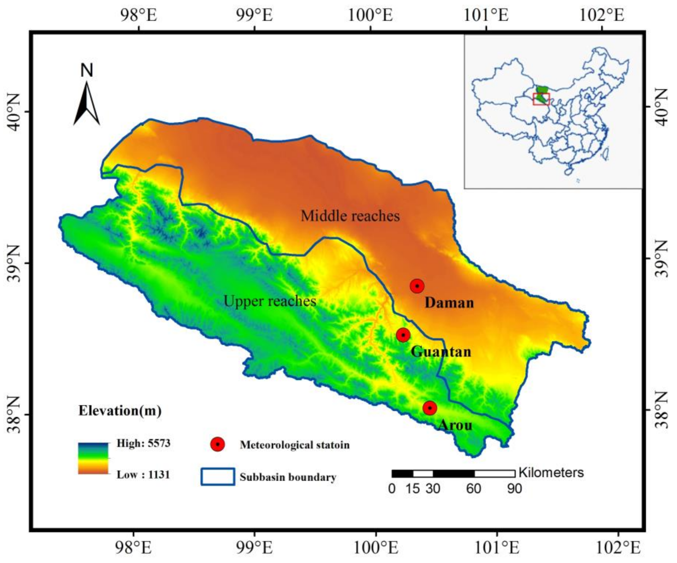
2.1. Site Description

In this study, data were collected from field automatic weather stations (AWSs) at three sites in the Heihe River basin distributed in the upper and middle reaches (Figure 1). Arou station is located in an east–west oriented valley with a maximum width of 3 km from north to south. The site is surrounded by natural alpine meadow with grass reaching a height of approximately 20–30 cm during the growing season. The Guantan site is surrounded by continuous mountains with elevations ranging from 2700–3400 m, and the weather station is located on the shady slope of the mountain in the Dayekou sub-catchment. The overstory tree species at the study site is Qinghai spruce, and the forest floor is nearly covered by a layer of moss with a depth of 10 cm [19]. Daman station is located in a typical oasis on very flat terrain near Zhangye City. The underlying surface is mainly irrigated maize that reaches a maximum height of approximately 180 cm [20].

2.2. Data

2.2.1. Onsite Data

The AWSs at these three sites collected 144 records per day including wind speed, wind direction, air temperature and air humidity at 10-min intervals at different heights. A description of the AWSs and the time periods covered by the data used in this study are listed in Table 1.

2.2.2. Satellite Data

Remotely sensed vegetation indices including the normalized difference vegetation index (NDVI) and leaf area index (LAI) were selected as the key indicators to measure the characteristic of vegetation growth. The time-series cloud-masked NDVI values of the sites were calculated using the MODIS red and infrared band reflectance after atmospheric correction: 2010 for the Guantan station and 2012 for the Arou station with 1 km resolution. The Savitzky–Golay (SG) filter was adopted to fill gaps to acquire the daily NDVI [21]. The 1-km/5-day composite LAI product in the Heihe River basin was acquired from the China science data centre (available online: http://card.westgis.ac.cn/), which consists of a normalization algorithm to integrate Terra-MODIS, Aqua-MODIS, FY3A-MERSI and FY3B-MERSI data. The time-continuous LAI were retrieved using neural networks and a maximum-value compositing algorithm [22,23,24].

3. Methods

3.1. Calculation of the Obukhov Length L

The Obukhov length L near the surface can be used to characterize the effect of atmospheric stability on the turbulence [25]. Therefore, this study investigates the implications of vertical measurement profiles in relation to the Monin–Obukhov similarity, using the gradient Richardson number (Ri) to infer L with the following equations:
L = { z /   Ri   when   R i < 0 z ( 1 5 Ri ) / Ri   when   R i > 0
where z = ( z 1 z 2 )/ln( z 1 / z 2 ) is the height where the calculated Richardson number is valid, z 1 is fixed at 10 m height, while z 2 is 2 m for Arou and Guantan site and 3 m for Daman site, respectively. Compared to L, Ri has the advantage that it contains only meteorological gradients that can be determined experimentally. Ri is expressed as the non-dimensional ratio between the buoyancy forces and the inertial ones due to the wind [26]. The sign of this number is determined by the temperature gradient, the negative values are an index of instability and the positive ones are an index of stability.
Ri = g ( θ v / z ) T ¯ ( u / z ) 2
where T ¯ is a reference atmospheric temperature, θ v / z is the difference in virtual potential temperature (VPT) between two measurements at heights z 1 and z 2 , g = 9.8   m / s 2 is the gravitational acceleration, and u / z is the wind gradient between z 1 and z 2 .

3.2. Calculating the Aerodynamic Roughness Length from AWS Data

To guarantee the reliability of the wind profile results, the raw datasets were pre-processed and quality control was performed to obtain aerodynamic roughness values based on the following criteria: (1) the minimum wind velocity of all layers exceeded 2 m/s; (2) data obtained at rainy times were discarded; (3) missing or invalid data were interpolated based on neighbouring data [18,27].
The aerodynamic surface roughness length can be determined iteratively based on wind profile data. Using the Monin–Obukhov similarity, the z0m values can be calculated via the logarithmic wind profile equation [6,7]:
u = u * k [ ln ( z d z 0 m ) Ψ m ( z d L ) ]
θ = θ * k [ ln ( z d z 0 h ) Ψ h ( z d L ) ] + θ 0
where u and θ denote the wind speed and potential air temperature, respectively, at the height z above ground level, u * is the friction velocity, θ * is the friction temperature; k is von Karman’s constant (k = 0.4); d is the zero-plane displacement; z 0 m is the aerodynamic roughness length; z 0 h is the thermal roughness length and θ 0 is the potential temperature near the surface. The expressions of the stability functions Ψ m   and   Ψ h depend on the stability conditions in the surface layer, which are described by the stability parameter Z/L [28].
When Z/L < 0 (unstable conditions) [29],
Ψ m   = ln 1 + x 2 2 + 2 ln 1 + x 2 2 arctgx + π 2
Ψ h = 2 ln 1 + y 2
x = ( 1 15 z d L ) 1 4 ,   y = ( 1 16 z d L ) 1 2
When Z/L > 0 (stable conditions) [30],
Ψ m   = Ψ h = 5 z d L
In this study, we use the least-squares method to determine z 0 m [31,32]. Equation (3) can be written as the following simplified form:
u = ax + b
where a = u * / k , x = ln ( z d ) Ψ m   and b = lnz 0 m · a . Commonly, d is related to the vegetation height (h) such that d equals 0.67 h over surfaces covered by dense and homogeneous vegetation [33]. Therefore, d is determined here by iterating over 0.1 m intervals of from 0.1 m to 3 m. For each given d, a correlation coefficient exists for the fitting Equation (9), and the optimal d value is chosen when the correlation coefficient reaches its maximum, the invalid value will be returned in loop iterations if the wind speed gradient is abnormal. Finally, the 10-min z0m values can be calculated according to the optimal d value. To maximally avoid effects from missing data, the z0m data are averaged over 30-min intervals and daily average z0m values are also calculated.

3.3. Correlation Analysis

Correlation coefficients measure the strength and direction of a relationship between two variables. Here, Pearson product–moment correlation coefficients were calculated to investigate the relationship between the latent factors and z0m. We selected the NDVI and the LAI as the most likely factors that represent the effects of vegetation growth on z0m and adopted wind speed (WS), wind direction ( θ ), relative humidity (RH), air temperature (T), Obukhov length (L) and air pressure (P) as the meteorological factors. Because Obukhov length is an instantaneous parameter that describes atmospheric conditions, calculating an average daily level of Obukhov length is meaningless and excluded from the correlation analysis of daily z0m. To match the half-hourly z0m data, we used daily NDVI and LAI values under the assumption that changes in vegetation indices can be ignored over shorter periods. Because wind direction is a categorical variable, we proposed a definition of wind deflection angle ( Δ θ ) between the prevailing wind direction ( θ p ) and the instantaneous wind direction, described as follows:
Δ θ = { | θ θ p |   when   | θ θ p | < 180 360 | θ θ p |   when   | θ θ p | > 180
The prevailing wind direction usually depends on the local topography, latitude and the locations of land and sea; therefore, Δ θ is categorized as a topographic factor in the subsequent factor analysis. The prevailing wind directions at the Arou, Guantan and Daman sites are 162°, 121° and 318° relative to due north, respectively, according to all observation data.

3.4. Factor Analysis

Factor analysis is a statistical method for decomposing input data as a linear combination of common factors and specific factors in a lower dimensional space. As a feature extraction approach, it seeks to acquire factor scores for input data in a lower dimensional space via a linear transformation. Those factor scores can be viewed as extracted features of the original data in another, lower-dimensional space. In this study, we first used correlation analysis to determine the main driving factors that influence the changes in z0m at half-hourly and daily intervals. Then, the main driving factors were normalized to eliminate the differences in dimensions between the variables:
X j = X j X j ¯ σ j
where X j is the indicator value of the j factor, and X j ¯ and σ j are the average and standard deviation of all the sample data of the j factor, respectively. Then, factor analysis was performed to determine the contributions of the vegetation indices and meteorological factors that affect z0m. The mathematical model of factor analysis is as follows [34]:
X k × 1 = A k × n F n × 1 + ε k × 1
where X = ( X 1 , X 2 , , X j , , X k ) is a k-dimensional stochastic vector composed of k samples, F = ( F 1 , F 2 , , F n ) is the common factor of X (n < k), ε k × 1 is an unobserved stochastic error factor with zero mean and finite variance and A k × n is the correlation coefficient matrix of the top n factors:
A k × n = [ a 11 a 1 n a k 1 a kn ] = [ u 11 λ 1 u 1 n λ n u k 1 λ 1 u kn λ n ]
where λ 1 , λ 2 , λ n are the first n characteristic values of the covariance matrix X k × 1 , and u 1 , u 2 , u n are the corresponding standard orthogonal eigenvectors. Based on the number of eigenvalues that exceed 1, the amounts of the common factors, n, can be determined. Then, the variance contribution of the common factor F n × 1 is obtained by calculating the sum of the squares of the elements in the j-th column of A k × n :
S j = i = 1 n a ij 2 ,   j = 1 , 2 , , n
which represents the sum of the variance contributions of the same common factor Fj to the variable. The cumulative contributions of the common factors can then be calculated accordingly. The factor analysis was performed using SPSS version 25 software (IBM, New York, NY, USA), using PCA as the extraction method and varimax as the rotation method.

4. Results

4.1. Driving Factors for Changes in Half-Hourly and Daily z0m

The results of bivariate correlation analyses between half-hourly z0m, daily z0m and each possible driving factor are shown in Table 2, which indicates that the main driving factors for z0m differ among the three stations. For the Arou and Guantan sites, the half-hourly and daily z0m values are positively correlated with the wind deflection angle and negatively correlated with the wind speed, while no significant correlation exists with the NDVI and the LAI, which represent the vegetative growth conditions. In contrast, at the Daman site, the half-hourly and daily z0m values are positively correlated with the NDVI and the LAI and negatively correlated with wind speed, while the wind deflection angle has no correlation to z0m. Similarly, half-hourly z0m is significantly correlated with the Obukhov length; however, neither half-hourly z0m nor daily z0m have any significant correlation with relative humidity, air temperature or air pressure at any of the sites. The factors that are significantly correlated with half-hourly z0m and those that are significantly correlated with daily z0m were selected to conduct a subsequent factor analysis. As Table 2 shows, only two factors have significant correlations with daily z0m at the Arou and Guantan sites; therefore, it is unnecessary to conduct a factor analysis. Consequently, we conducted the factor analysis for daily z0m only at the Daman site and for half-hourly z0m at all three sites.

4.2. Contributions of Driving Factors to Half-Hourly z0m

Before conducting the factor analysis, Kaiser–Meyer–Olkin (KMO) [35] and Bartlett’s sphericity tests [36] were applied to examine the appropriateness of the data for factor analysis. The KMO test determines the degree of correlation between variables with partial correlation coefficients: the KMO values for the half-hourly z0m values at the Arou, Guantan and Daman sites were 0.625, 0.591 and 0.703, respectively, all of which satisfy the minimal requirement; that is, they are above 0.5. Bartlett’s sphericity test determines whether variables are independent based on the variables’ correlation coefficient matrixes. The Bartlett’s sphericity test results were 67.222, 58.761 and 121.928 at the Arou, Guantan and Daman sites, respectively, and the p-value for each site was 0: all of these satisfy the requirement that p should be below 0.001. Based on the results of these two tests, the data are suitable for factor analysis.
Table 3 and Table 4 show the factor analysis results. For half-hourly z0m at the Arou and Guantan sites, the first common factors are wind speed and Obukhov length, which are aerodynamic factors (A_factor): their contributions for Arou and Guantan are 44.03% and 42.87%, respectively. The second common factor (the topographic factor (T_factor)) is mainly expressed by wind deflection angle, and the contributions at Arou and Guantan are 38.33% and 38.66%, respectively. For the Daman site, the first common factor is the vegetation factor (V_factor) consisting of NDVI and LAI: the factor loads for NDVI and LAI are 0.959 and 0.941, respectively. The contribution of the vegetation factor is 53.14%. The aerodynamic factor, composed of wind speed and Obukhov length, is a secondary factor that contributes of 30.29%.

4.3. Contributions of Driving Factors to Daily z0m

The KMO value for daily z0m at the Daman site is 0.731, which satisfies the minimal requirement (>0.5). The Bartlett’s sphericity test value is 333.777 and the p value is 0. Both the KMO test and Bartlett’s sphericity test demonstrate the feasibility of the data for factor analysis. Similar to the results of half-hourly z0m, the first common factor for daily z0m at the Daman site is the vegetation factor, which is composed of NDVI and LAI with factor loads of 0.969 and 0.960, respectively. The contribution of the vegetation factor is 54.46%. The contribution of the aerodynamic factor is 30.67%.

5. Discussion

5.1. The Applicability of Monin–Obukhov Similarity

In this research, we adopted a traditional method of calculating observed z0m by fitting the profile observations using Monin–Obukhov similarity (MOS). As MOS was developed under homogeneous and flat underlying conditions, the applicability of MOS at the Arou and Guantan sites, which are located in mountainous areas, needs to be examined further. We filter the profiles with minimum wind velocity over 1 m/s and separate the wind speed data of one certain layer (20 m at the Arou site and 2 m at the Guantan site) as the target for validation. The remainder of the profiles are used to calculate the friction velocity, the displacement height and the aerodynamic roughness length in the MOS framework. Then, the wind speed of the target layer can be calculated accordingly. Figure 2 shows the linear fitting relationships between the measured wind speed and the calculated wind speed of the target layer: the coefficients of determination (R2) values of the fitted equations are 0.95 and 0.68 for the Arou site and the Guantan site, respectively, indicating significant relationships between the measured wind speed and the calculated wind speed at both sites, confirming the applicability of MOS.

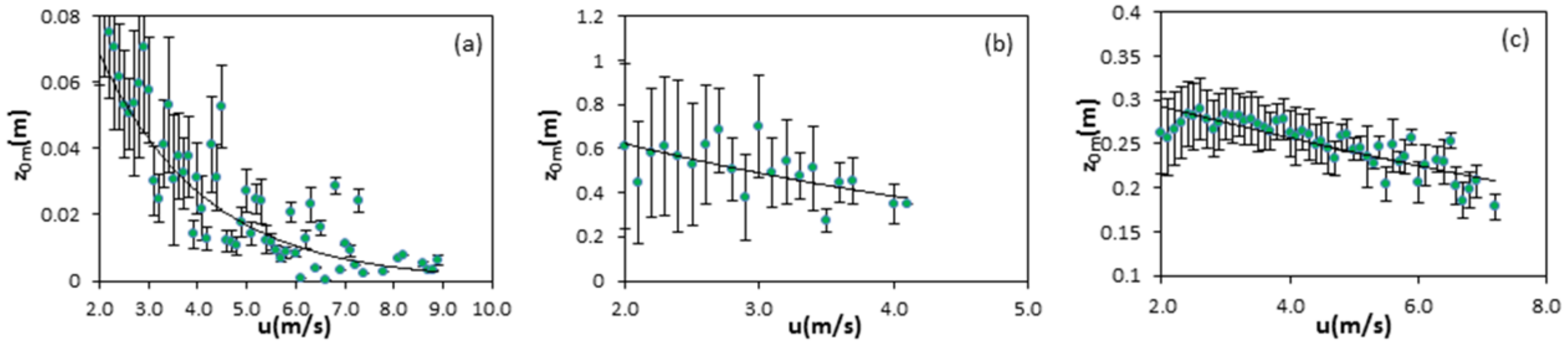
5.2. The Wind Speed Factor

To formulate the detailed change rule between z0m and wind speed, we select the measured AWS data in August, when the vegetation reaches its peak-growth stage. The averaged z0m values and standard deviations are calculated at 0.1 m/s wind speed intervals. Figure 3 reveals that the z0m values decrease with increasing wind speed. The reduction in z0m as the wind speed increases is most significant at the Arou site, and to a certain extent, the z0m values remain relatively low and stable when the wind speeds become high (Figure 3a). Because of the barrier effects of the densely distributed stands of spruce around the Guantan site, the maximum wind speed in August is just over 4 m/s; thus, the descending z0m trend is not pronounced (Figure 3b). At the Daman site, z0m has a slowly descending tendency that is significantly correlated with increased wind speeds (Figure 3c). At slow wind speeds, the standard deviations of z0m at all the stations are generally larger, possibly because the weak wind creates irregular turbulence inside the vegetation, resulting in large variations of z0m under similar wind speed conditions.
The most likely explanations for the decrease in aerodynamic roughness with increasing wind speed are as follows: as the wind speed increases, the wind changes the geometry of nonrigid bodies (such as vegetation) above the ground surface to some extent. In other words, as the stalks or blades of a plant lean in the same direction under wind action, the airflow drag due to the rough elements decreases; as the wind speed continues to increase, there is a critical point at which the plants reach equilibrium and their shapes no longer change with the wind speed. When the observed wind speed is small, the z0m measured at the Guantan and Daman sites never reach this stable stage, whereas, at Arou, the z0m measurements reflect this equilibrium.

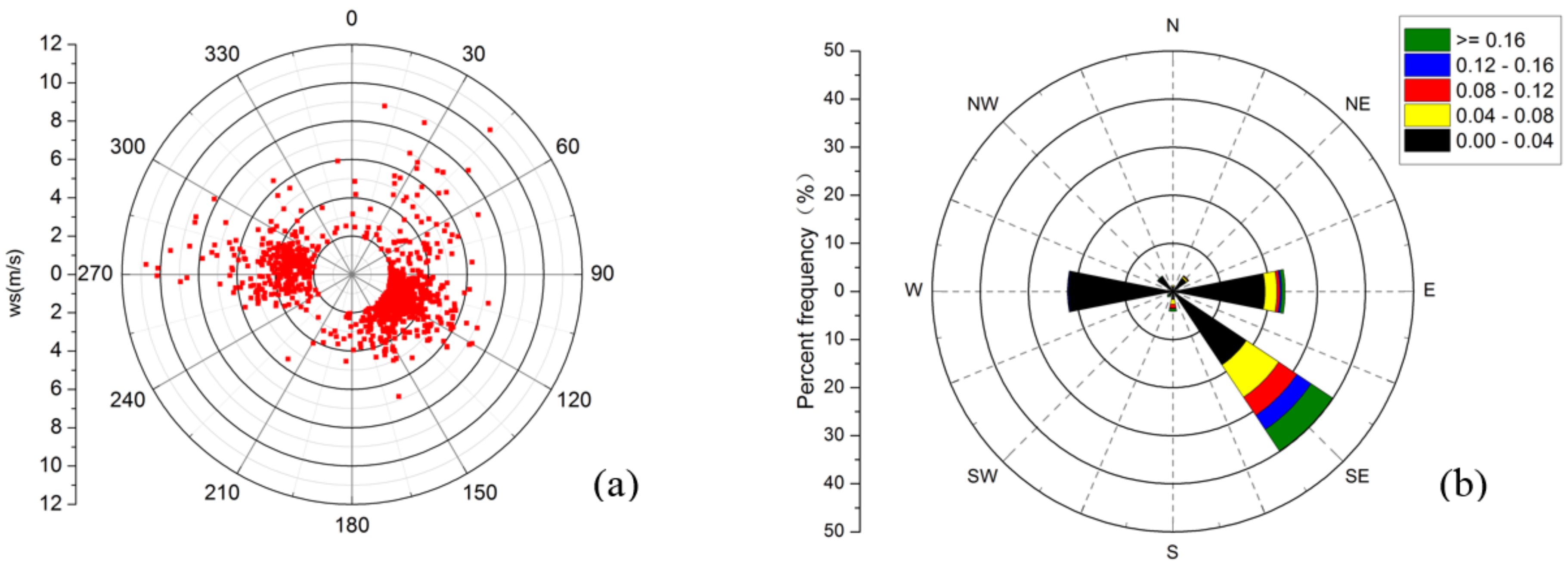
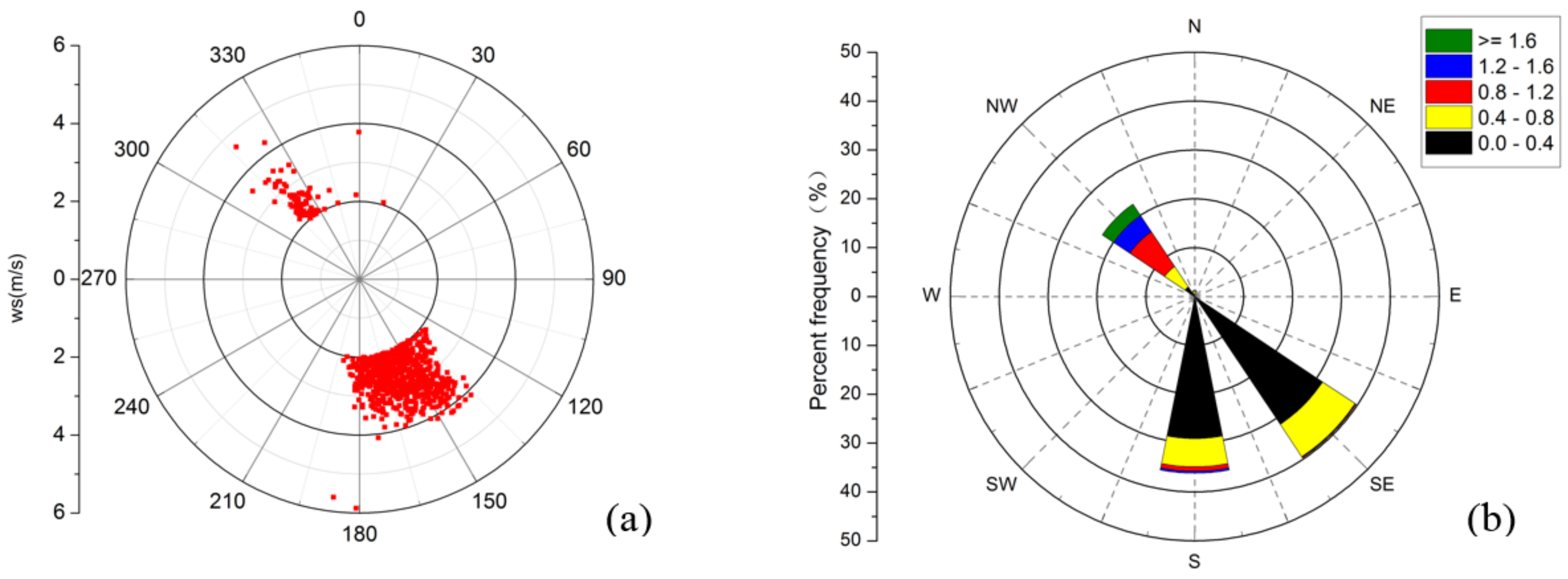
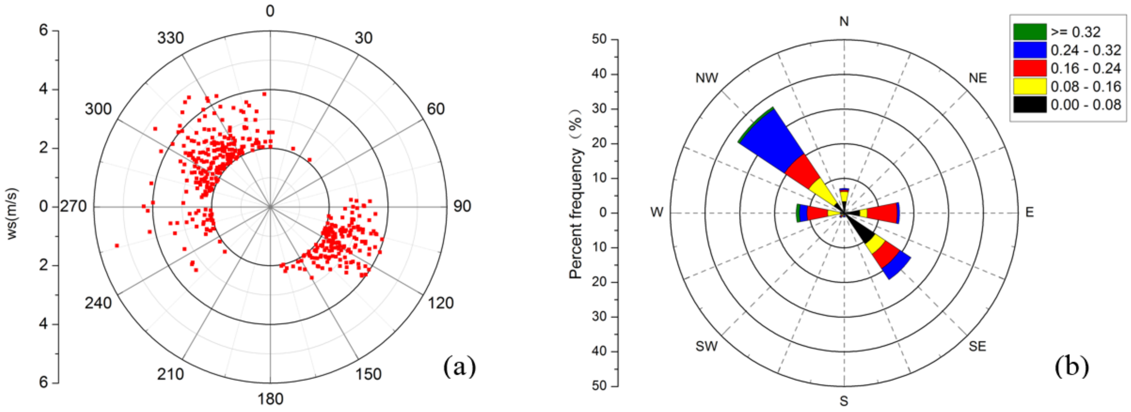
5.3. The Wind Direction Factor

The influence of wind direction under unstable conditions was also explored to assess the homogeneity of these three sites. We plotted the distributions of half-hourly wind speed under different wind directions on polar coordinates; the frequency percentages of z0m were classified at eight common wind directions (N-NE-E-SE-S-SW-W-NW). As Figure 4a shows, the dominant prevailing winds are west and southeast at the Arou site. Although the wind speed values are similar, significant differences occur in the z0m between these two wind directions (Figure 4b): under a west wind, 98% of the z0m values are less than 0.04 m, while under a southeast wind, 58% of the z0m values under exceed 0.04 m. Therefore, easterly winds tend to result in larger z0m values at the Arou site. At the Guantan site, wind is concentrated in two opposite directions, which can be partially explained by the mountains around the site. The z0m values under the different wind directions also vary significantly (Figure 5b). Under south and southeast winds, approximately 80% of the z0m values are less than 0.4 m. In contrast, under a northwest wind, 90% of the z0m values are greater than 0.4 m. These results occur because the Guantan site is located on the shady slope of the mountain; thus, wind blowing directly against the slope results in larger z0m values. The Daman site is located in an irrigated flat farm area where the topography has little influence on the wind. The prevailing wind directions in August are southeast and northwest, and there is no significant difference in the frequency distribution of z0m between the different wind directions, as shown in Figure 6b.
Table 5 shows the mean values of z0m in August calculated at the two prevailing wind directions at each site and shows that the z0m values at Arou and Guantan site differ significantly with wind direction, while those at the Daman site are similar even under two opposite wind directions. Considering that the topographic relief of the entire source area is more prominent at Arou and Guantan sites compared with that at the Daman site, the z0m influences from changes in wind direction may depend on the heterogeneity of the topography. For areas with complicated terrain, the density and distribution of rough elements presented to each wind direction differ; therefore, the drag forces near the earth's surface also differ, resulting in z0m variations under different wind directions. However, in the area surrounding the Daman site, maize crops are planted in the homogeneous underlying surface; the densely distributed plants tend to flatten the small rough elements, leading to few z0m effects from wind direction. In conclusion, wind direction is a main driving factor for z0m in mountainous areas but can be ignored when modelling z0m over flat surfaces underlying homogenous vegetation.

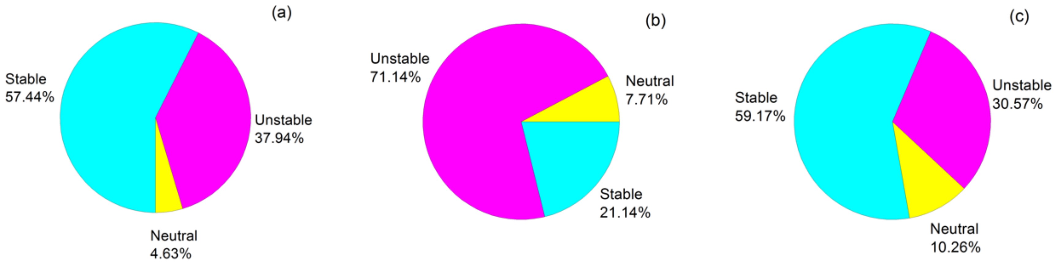
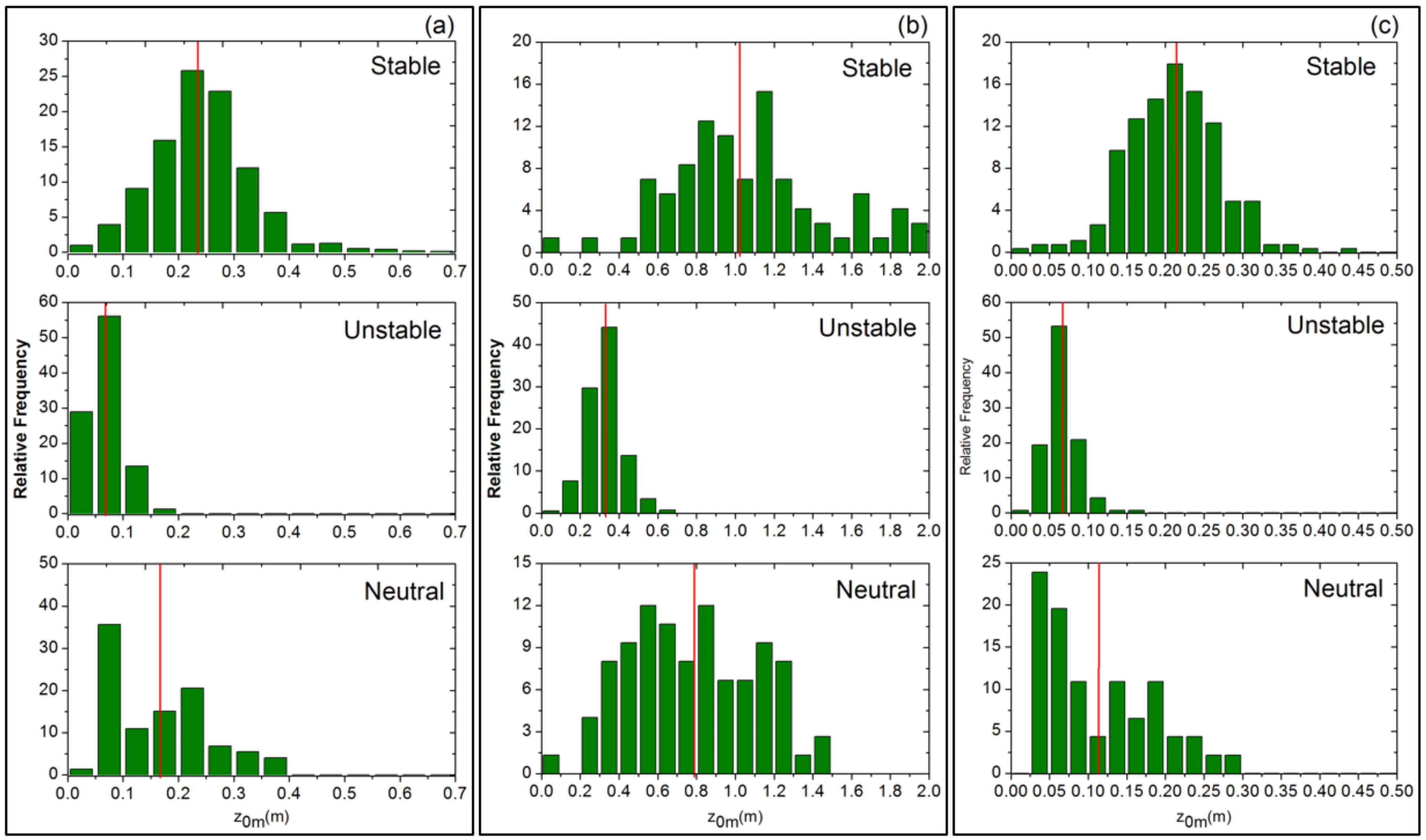
5.4. The Atmospheric Stability Factor

In previous studies, most researchers tend to filter z0m under neutral conditions to simplify the z0m estimation models, which are built on the assumption that z0m under neutral conditions can represent the average level and that z0m is not significantly different under different atmospheric conditions. However, based on the results of our factor analysis, this assumption might be incorrect. As listed in Table 6, the Obukhov lengths are binned by stability class to simplify analysis. Although the definition of the stability bins varies with local environmental conditions, these definitions have previously been used by authors [37,38]. The different atmospheric stability conditions in August are counted and presented by the frequency pie chart in Figure 7. The stable condition percentage is highest at the Arou and Daman sites, while unstable conditions form the highest proportion at the Guantan site. However, the neutral condition comprises only a small portion of all sites; therefore, the z0m value under the neutral condition is not representative, especially for instantaneous flux calculations.
Figure 8 shows the distribution of half-hourly z0m in August for stable, unstable and neutral conditions. Obviously, z0m presents clear differences under different stability conditions at each site. Because neutral conditions accounted for the smallest percentage, there are not enough samples to ensure that z0m is normally distributed under these conditions. A comparison of these results shows that the averaged z0m under stable conditions has the highest value, followed by that under neutral conditions, and the lowest values appear under unstable conditions. Under stable conditions, the z0m values have a border value range and are distributed in a nearly normal fashion. Actually, atmospheric stability is closely related to the alternation of day and night. In the daytime, affected by the solar radiation, turbulent exchanges occur frequently between vegetation and the atmosphere and unstable atmospheric conditions are prominent; therefore, z0m maintains low levels. At night, the atmospheric turbulence weakens, and z0m increases significantly under the more stable conditions. In addition, because the relative frequencies of z0m are similarly distributed among these three sites, we deduce that the influence on z0m caused by atmospheric stability has nothing to do with the underlying surface.

6. Conclusions

This study statistically investigated the driving factors that influence z0m at different time scales using three AWSs in the Heihe river basin that collect data for different land surface patterns. Aerodynamic factors, including wind speed and Obukhov length, are the main driving forces for the half-hourly changes in z0m at the Arou Site and Guantan site, contributing 44.03% and 42.87%, respectively, at those sites, while topographic factors linked to the wind deflection angle contribute 38.33% and 38.66% to the half-hourly changes in z0m at the two sites, respectively. Regarding the daily z0m at the Arou and Guantan sites, only wind speed and wind deflection angle are correlating factors. The driving factors for half-hourly z0m at the Daman site include both vegetation and aerodynamic factors, with contributions of 53.14% and 30.29%, respectively. Similar results were found for the daily z0m at Daman site, except that atmospheric stability was not considered. It should be noted that vegetation factors such as NDVI and LAI have no significant relationship with either the half-hourly z0m or the daily z0m at the Arou and Guantan sites, but these vegetation factors are the primary driving factors for the Daman site, probably because of fewer changes in the botanical characteristics of grass and forest over growing seasons compared with the rapid changes due to crop growth in farmland. Researchers should recognize that meteorological factors cannot be neglected in z0m estimation models, especially for instantaneous flux simulations.
However, there are still some uncertainties in the results. First, this study focused only on the changes of z0m during the vegetative growth period; consequently, which factors are most influential in other seasons is still unclear. Second, the factors tested in this paper are not comprehensive due to data source limitations; therefore, more factors that may influence z0m should be taken into account. Third, the displacement height d, as the other important roughness parameter, is discussed relatively little in this paper; and the correlation between instantaneous d and z0m may influence the accuracy of the observed z0m. Thus, the driving factors of d and z0m need to be examined at more sites with a wider variety of underlying surface and climate features to improve the robustness of the conclusions.

Acknowledgments

This work was supported by National Key R&D Program of China (No. 2016YFA0600304) and the Advanced Science Foundation Research Project of the Chinese Academy of Sciences (Grant No.: QYZDY-SSW-DQC014). The authors thank the Environmental and Ecological Science Data Center for West China, National Natural Science Foundation of China for providing the AWS data (http://westdc.westgis.ac.cn).

Author Contributions

Mingzhao Yu contributed to the research experiments, analysed the data, and wrote the paper. Bingfang Wu conceived the experiments, and was responsible for the research analysis. Hongwei Zeng, Qiang Xing and Weiwei Zhu collected and pre-processed the original data. All the co-authors helped to revise the manuscript.

Conflicts of Interest

The authors declare no conflict of interest.

References

  1. Stull, R.B. An Introduction to Boundary Layer Meteorology. Atmos. Sci. Libr. 1988, 8, 89. [Google Scholar]
  2. Hryama, T.; Sugita, M.; Kotoda, K. Regional Roughness Parameters and Momentum Fluxes over a Complex Area. J. Appl. Meteorol. 1996, 35, 336–347. [Google Scholar] [CrossRef]
  3. Marticorena, B.; Kardous, M.; Bergametti, G.; Callot, Y.; Chazette, P.; Khatteli, H.; Le Hégarat-Mascle, S.; Maillé, M.; Rajot, J.; Vidal-Madjar, D.; et al. Surface and aerodynamic roughness in arid and semiarid areas and their relation to radar backscatter coefficient. J. Geophys. Res. Earth Surf. 2006, 111. [Google Scholar] [CrossRef] [Green Version]
  4. Monteith, J.L. The micrometeorology of crops. In Principles of Environmental Physics; Edward Arnold: London, UK, 1973; pp. 190–215. [Google Scholar]
  5. Brutsaert, W. Evaporation into the Atmosphere; Theory, History, and Applications; Springer: Dordrecht, The Netherlands, 1982. [Google Scholar]
  6. Raupach, M.R. Drag and drag partition on rough surfaces. Bound. Layer Meteorol. 1992, 60, 375–395. [Google Scholar] [CrossRef]
  7. Raupach, M. Simplified expressions for vegetation roughness length and zero-plane displacementas functions of canopy height and area index. Bound. Layer Meteorol. 1994, 71, 211–216. [Google Scholar] [CrossRef]
  8. Schmid, H.P.; Bünzli, B. The influence of surface texture on the effective roughness length. Q. J. R. Meteorol. Soc. 1995, 121, 1–21. [Google Scholar] [CrossRef]
  9. Gupta, R.K.; Prasad, T.S.; Vijayan, D. Estimation of roughness length and sensible heat flux from WiFS and NOAA AVHRR data. Adv. Sp. Res. 2002, 29, 33–38. [Google Scholar] [CrossRef]
  10. Choudhury, B.J.; Monteith, J.L. A four-layer model for the heat budget of homogeneous land surfaces. Q. J. R. Meteorol. Soc. 1988, 114, 373–398. [Google Scholar] [CrossRef]
  11. Yu, M.; Wu, B.; Yan, N.; Xing, Q.; Zhu, W. A Method for Estimating the Aerodynamic Roughness Length with NDVI and BRDF Signatures Using Multi-Temporal Proba-V Data. Remote Sens. 2016, 9, 6. [Google Scholar] [CrossRef]
  12. Colin, J.; Menenti, M.; Rubio, E.; Jochum, A. Accuracy vs. Operability: A Case Study over Barrax in the Context of the DEMETER Project. AIP Conf. Proc. 2006, 852, 75–83. [Google Scholar]
  13. Jasinski, M.F.; Borak, J.; Crago, R. Bulk surface momentum parameters for satellite-derived vegetation fields. Agric. For. Meteorol. 2005, 133, 55–68. [Google Scholar] [CrossRef]
  14. Zhou, Y.L.; Sun, X.M.; Zhang, R.H.; Zhu, Z.L.; Xu, J.P.; Li, Z.L. The improvement and validation of the model for retrieving the effective roughness length on TM pixel scale. In Proceedings of the IEEE International Geoscience and Remote Sensing Symposium, Seoul, Korea, 25–29 July 2005; pp. 3059–3062. [Google Scholar]
  15. Zhou, Y.L. Surface Roughness Length Dynamic and Its Effects on Fluxes Simulation. Ph.D. Thesis, Institute of Geographic Sciences and Natural Resources Research, CAS, Beijing, China, 2008. [Google Scholar]
  16. Gao, Y.; Hu, Y. Advances in HEIFE Research (1987–1994); China Meteorological Press: Beijing, China, 1994. [Google Scholar]
  17. Li, X.; Li, X.W.; Li, Z.; Ma, M.; Wang, J.; Xiao, Q.; Liu, Q.; Che, T.; Chen, E.; Yan, G.; et al. Watershed allied telemetry experimental research. J. Geophys. Res. Atmos. 2009, 114, 2191–2196. [Google Scholar] [CrossRef]
  18. Liu, X.; Cheng, G.D.; Liu, S.M.; Xiao, Q.; Ma, M.; Jin, R.; Che, T.; Liu, Q.; Wang, W.; Qi, Y.; et al. Heihe watershed allied telemetry experimental research (Hiwater): Scientific objectives and experimental design. Bull. Am. Meteorol. Soc. 2013, 94, 1145–1160. [Google Scholar] [CrossRef]
  19. Mingguo, M.; Weizhen, W.; Junlei, T.; Guanghui, H.; Zhihui, Z. WATER: Dataset of Automatic Meteorological Observations at the Dayekou Guantan Forest Station in the Dayekou Watershed; Cold and Arid Regions Environmental and Engineering Research Institute, Chinese Academy of Sciences: Beijing, China, 2008. [Google Scholar]
  20. Liu, S.M.; Xu, Z.W.; Wang, W.Z.; Jia, Z.Z.; Zhu, M.J.; Bai, J.; Wang, J.M. A comparison of eddy-covariance and large aperture scintillometer measurements with respect to the energy balance closure problem. Hydrol. Earth Syst. Sci. 2011, 15, 1291–1306. [Google Scholar] [CrossRef]
  21. Chen, J.; Jönsson, P.; Tamura, M.; Gu, Z.; Matsushita, B.; Eklundh, L. A simple method for reconstructing a high-quality NDVI time-series data set based on the Savitzky-Golay filter. Remote Sens. Environ. 2004, 91, 332–344. [Google Scholar] [CrossRef]
  22. Yin, G.; Li, J.; Liu, Q.; Fan, W.; Xu, B.; Zeng, Y.; Zhao, J. Regional Leaf Area Index Retrieval Based on Remote Sensing: The Role of Radiative Transfer Model Selection. Remote Sens. 2015, 7, 4604–4625. [Google Scholar] [CrossRef]
  23. Yin, G.; Li, J.; Liu, Q.; Zhong, B.; Li, A. Improving LAI spatio-temporal continuity using a combination of MODIS and MERSI data. Remote Sens. Lett. 2016, 7, 771–780. [Google Scholar] [CrossRef]
  24. Li, X.; Liu, S.M.; Xiao, Q.; Ma, M.G.; Jin, R.; Che, T.; Wang, W.Z.; Hu, X.L.; Xu, Z.W.; Wen, J.G.; et al. A multiscale dataset for understanding complex eco-hydrological processes in a heterogeneous oasis system. Sci. Data 2017, 4, 170083. [Google Scholar] [CrossRef] [PubMed]
  25. Argyle, P.; Watson, S.J. Assessing the dependence of surface layer atmospheric stability on measurement height at offshore locations. J. Wind Eng. Ind. Aerodyn. 2014, 131, 88–99. [Google Scholar] [CrossRef] [Green Version]
  26. Richardson, L.F. Some Measurements of Atmospheric Turbulence. R. Soc. 1921, 221, 582–593. [Google Scholar] [CrossRef]
  27. Zhu, W.; Wu, B.; Yan, N.; Feng, X.; Xing, Q. A method to estimate diurnal surface soil heat flux from MODIS data for a sparse vegetation and bare soil. J. Hydrol. 2014, 511, 139–150. [Google Scholar] [CrossRef]
  28. Panofsky, H.A. Determination of stress from wind and temperature measurement. Q. J. R. Meteorol. Soc. 1963, 89, 85–94. [Google Scholar] [CrossRef]
  29. Dyer, A.J. A review of flux-profile relationships. Bound. Layer Meteorol. 1974, 7, 363–372. [Google Scholar] [CrossRef]
  30. Webb, E.K. Profile relationships: The log-linear range, and extension to strong stability. Q. J. R. Meteorol. Soc. 1970, 96, 67–90. [Google Scholar] [CrossRef]
  31. Frangi, J.P.; Richard, D.C. The WELSONS experiment: Overview and presentation of first results on the surface atmospheric boundary-layer in semiarid Spain. Ann. Geophys. 2000, 18, 365–384. [Google Scholar] [CrossRef]
  32. Zhou, Y.; Ju, W.; Sun, X.; Wen, X.; Guan, D. Significant decrease of uncertainties in sensible heat flux simulation using temporally variable aerodynamic roughness in two typical forest ecosystems of China. J. Appl. Meteorol. Climatol. 2012, 51, 1099–1110. [Google Scholar] [CrossRef]
  33. Pielke, S.; Roger, A. Mesoscale Meteorological Modeling; Academic Press: Cambridge, MA, USA, 2013; Volume 98. [Google Scholar]
  34. Zou, M.; Niu, J.; Kang, S.; Li, X.; Lu, S. The contribution of human agricultural activities to increasing evapotranspiration is significantly greater than climate change effect over Heihe agricultural region. Sci. Rep. 2017, 7, 8805. [Google Scholar] [CrossRef] [PubMed]
  35. Kaiser, H.F. An index of factorial simplicity. Psychometrika 1974, 39, 31–36. [Google Scholar] [CrossRef]
  36. Bartlett, M.S. Properties of Sufficiency and Statistical Tests. Proc. R. Soc. Lond. 1937, 160, 268–282. [Google Scholar] [CrossRef]
  37. Motta, M.; Barthelmie, R.J.; Vølund, P. The influence of non-logarithmic wind speed profiles on potential power output at Danish offshore sites. Wind Energy 2005, 8, 219–236. [Google Scholar] [CrossRef]
  38. Muñozesparza, D.; Cañadillas, B.; Neumann, T.; van Beeck, J. Turbulent fluxes, stability and shear in the offshore environment: Mesoscale modelling and field observations at FINO1. J. Renew. Sustain. Energy 2012, 4, 063136. [Google Scholar] [CrossRef]
Figure 1. Locations of the three automatic weather stations (AWSs) in the Heihe River basin. The elevation map was produced using the ASTER GDEM product of METI and NASA (available online: http://www.gdem.aster.ersdac.or.jp).
Atmosphere 09 00149 g001
Figure 2. The distribution of scatters at (a) Arou site and (b) Guantan site between measured wind speed and calculated wind speed with Monin–Obukhov (MOS).
Atmosphere 09 00149 g002
Figure 3. Distribution of half-hourly z0m under variant wind speed scope at (a) Arou station; (b) Guantan station and (c) Daman station. Error bars centred at each data point indicate 95% confidence intervals of the regression estimate; an exponential trend line is added for each data series.
Atmosphere 09 00149 g003
Figure 4. (a) Distribution map of half-hourly wind speed data and (b) half-hourly z0m rose-binned data map at Arou station in August.
Atmosphere 09 00149 g004
Figure 5. (a) Distribution map of half-hourly wind speed data and (b) half-hourly z0m rose-binned data map at Guantan station in August.
Atmosphere 09 00149 g005
Figure 6. (a) Distribution map of half-hourly wind speed data and (b) half-hourly z0m rose-binned data map at Daman station in August.
Atmosphere 09 00149 g006
Figure 7. Frequency pie chart of different stabilities at the (a) Arou site; (b) Guantan site and (c) Daman site.
Atmosphere 09 00149 g007
Figure 8. Relative frequency of z0m for stable, unstable and neutral conditions at the (a) Arou site; (b) Guantan site and (c) Daman site. The vertical red lines in each image indicate the mean values.
Atmosphere 09 00149 g008
Table 1. Description of the three used AWSs.
LocationCoordinatesAltitude (m)Land UseSensor Height (m)PeriodData Logger
Arou38°2′50′′ N,
100°27′51′′ E
3033Alpine meadow1, 2, 5, 10, 15, 251 May 2014–31 October 2014CR23X
Guantan38°32′1′′ N,
100°15′0′′ E
2835Qinghai spruce2, 10, 241 May 2011–31 October 2011CR23XTD
Daman38°51′20′′ N,
100°22′20′′ E
1556Spring maize3, 5, 10, 15, 20, 30, 401 May 2014–31 October 2014CR800
Table 2. The correlation coefficients (R) between half-hourly z0m, daily z0m and possible driving factors.
FactorsArou z0mGuantan z0mDaman z0m
Half-HourlyDailyHalf-Hourly DailyHalf-Hourly Daily
WS−0.592 **−0.488 **−0.409 **−0.326 *−0.326 *−0.345 *
Δ θ 0.574 **0.641 **0.725 **0.407 **0.0270.123
RH0.2740.0400.1370.0930.0110.061
T−0.125−0.2000.2230.1800.1490.263
L0.608 **-0.602 **-0.542 **-
P0.1130.0790.2760.1510.0090.056
NDVI0.1610.2820.0180.1300.546 **0.639 **
LAI0.0810.177−0.0690.0520.571 **0.671 **
An asterisk (*) denotes a correlation significant at the 0.05 level; A double asterisk (**) denotes a correlation significant at the 0.01 level.
Table 3. Rotated component matrix in factor analysis.
FactorsArou Half-HourlyGuantan Half-HourlyDaman Half-HourlyDaman Daily
A_FactorT_Factor A_FactorT_Factor V_FactorA_FactorV_FactorA_Factor
WS−0.765−0.003−0.799−0.232−0.239−0.514−0.350−0.667
Δ θ −0.0420.998−0.0260.829----
L0.764−0.0520.6620.0950.0100.973--
NDVI----0.959−0.0680.969−0.023
LAI----0.941−0.0580.960−0.047
Table 4. The contributions of factors for z0m.
SiteItemsComponentRotation Sums of Squared Loadings
Eigen ValueVariance Contribution (%)Cumulative Variance Contribution (%)
ArouHalf-hourly z0mA_factor1.97144.0344.03
T_factor1.20238.3382.36
GuantanHalf-hourly z0mA_factor1.70642.8742.87
T_factor1.28038.6681.53
DamanHalf-hourly z0mV_factor2.12553.1453.14
A_factor1.05230.2983.43
Daily z0mV_factor2.17854.4654.46
A_factor1.05730.6785.13
Table 5. Statistical table of averaged z0m under prevailing wind direction.
z 0 m ¯ ArouGuantanDaman
primary wind direction0.072(SE)0.349(SE)0.237(NW)
secondary wind direction0.009(W)1.021(NW)0.215(SE)
Table 6. Classification of atmospheric stability.
Atmospheric ConditionDefinition
Stable0 < L < 1000
Unstable−1000 < L < 0
NeutralL < −1000 or L > 1000

