Seasonal Variability of Airborne Particulate Matter and Bacterial Concentrations in Colorado Homes


Abstract
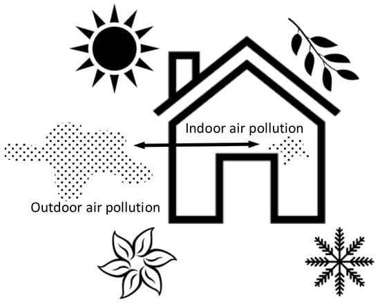
1. Introduction
2. Methods
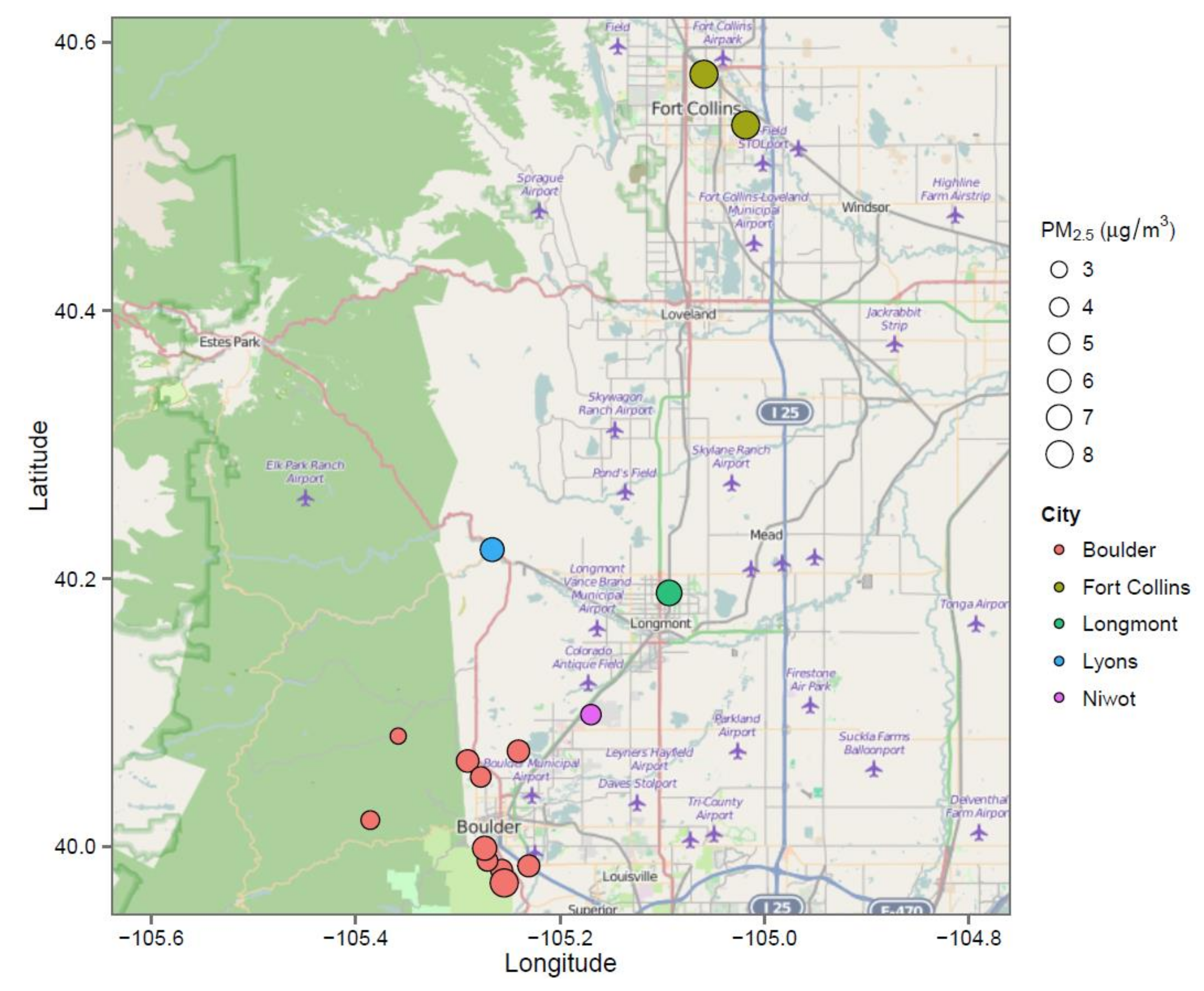
2.1. Study Home Characteristics
2.2. Instrumentation and Metadata Collection
2.3. Data Analyses
3. Results and Discussion
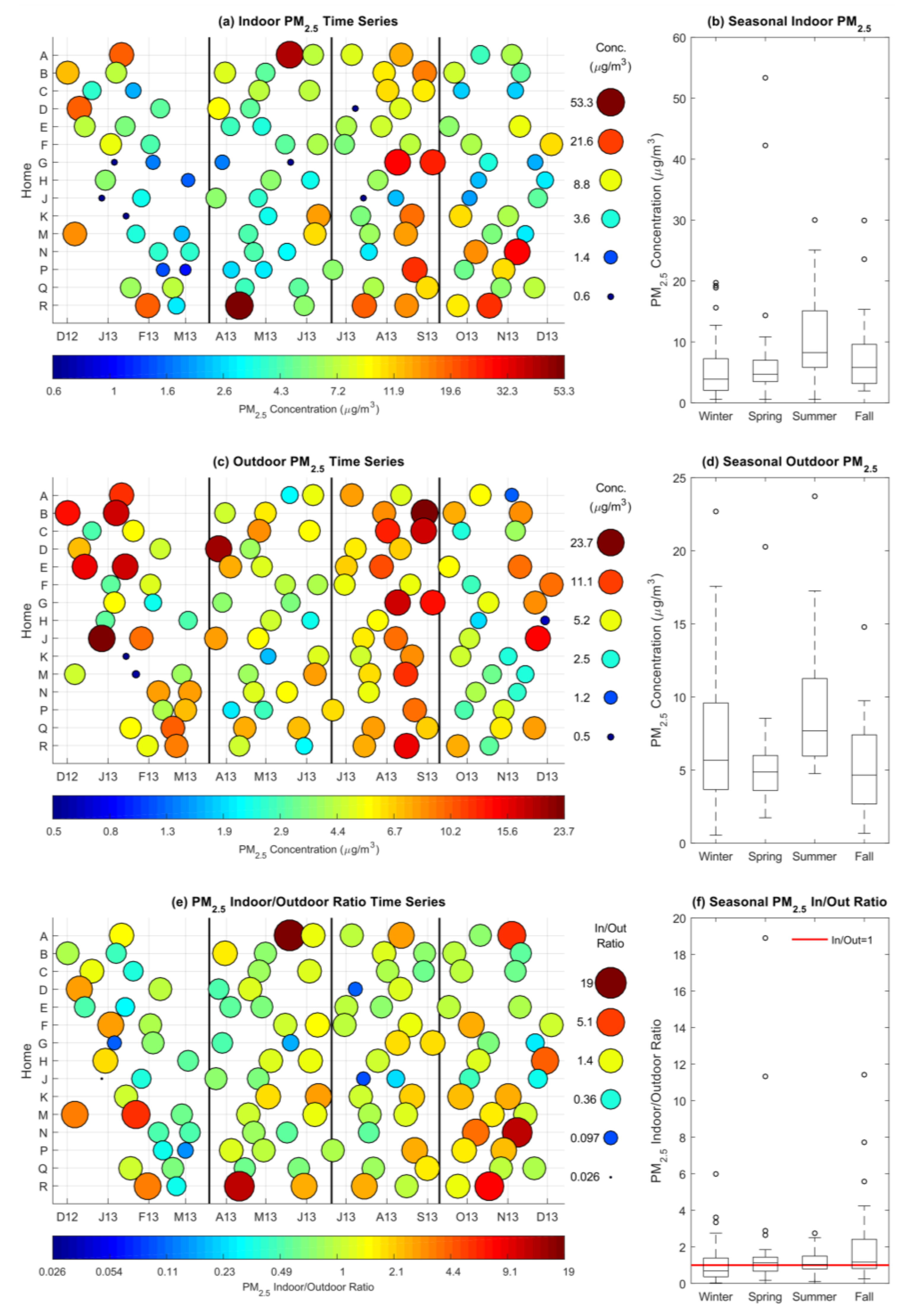
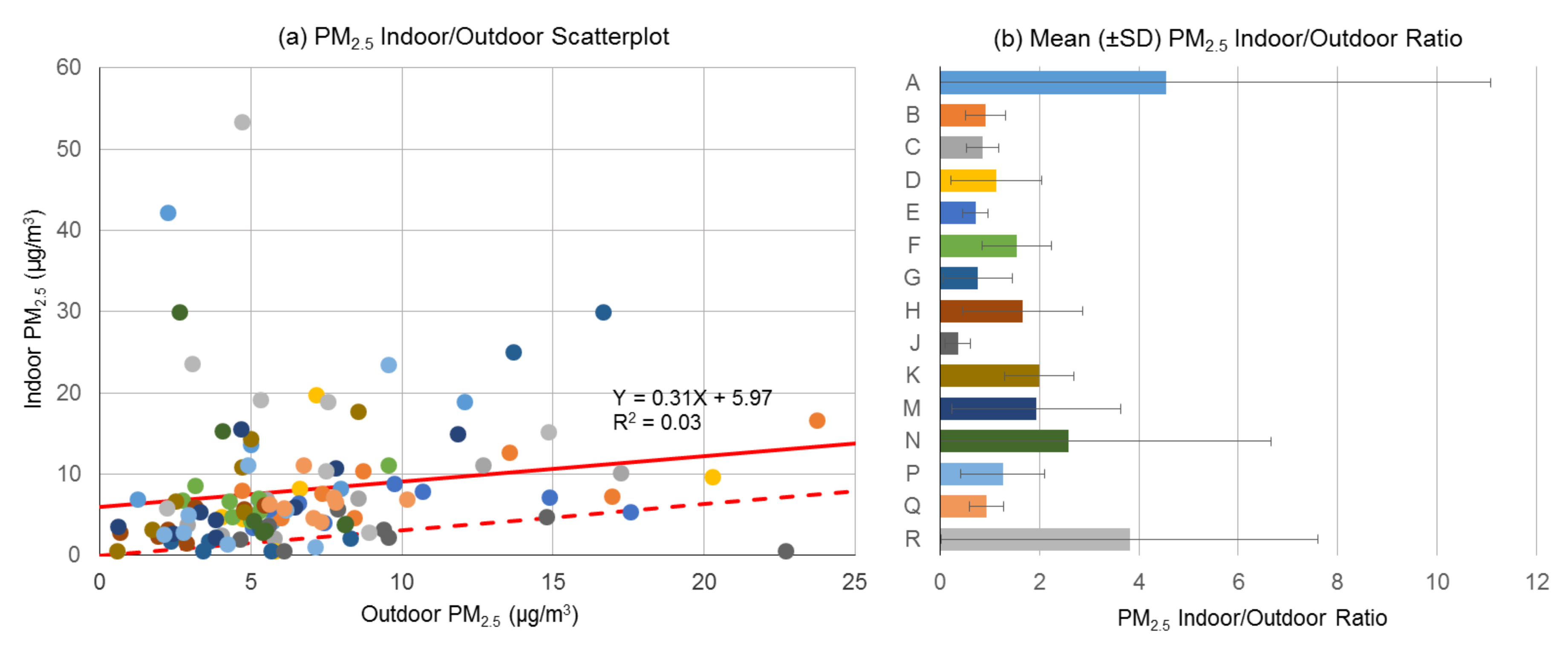
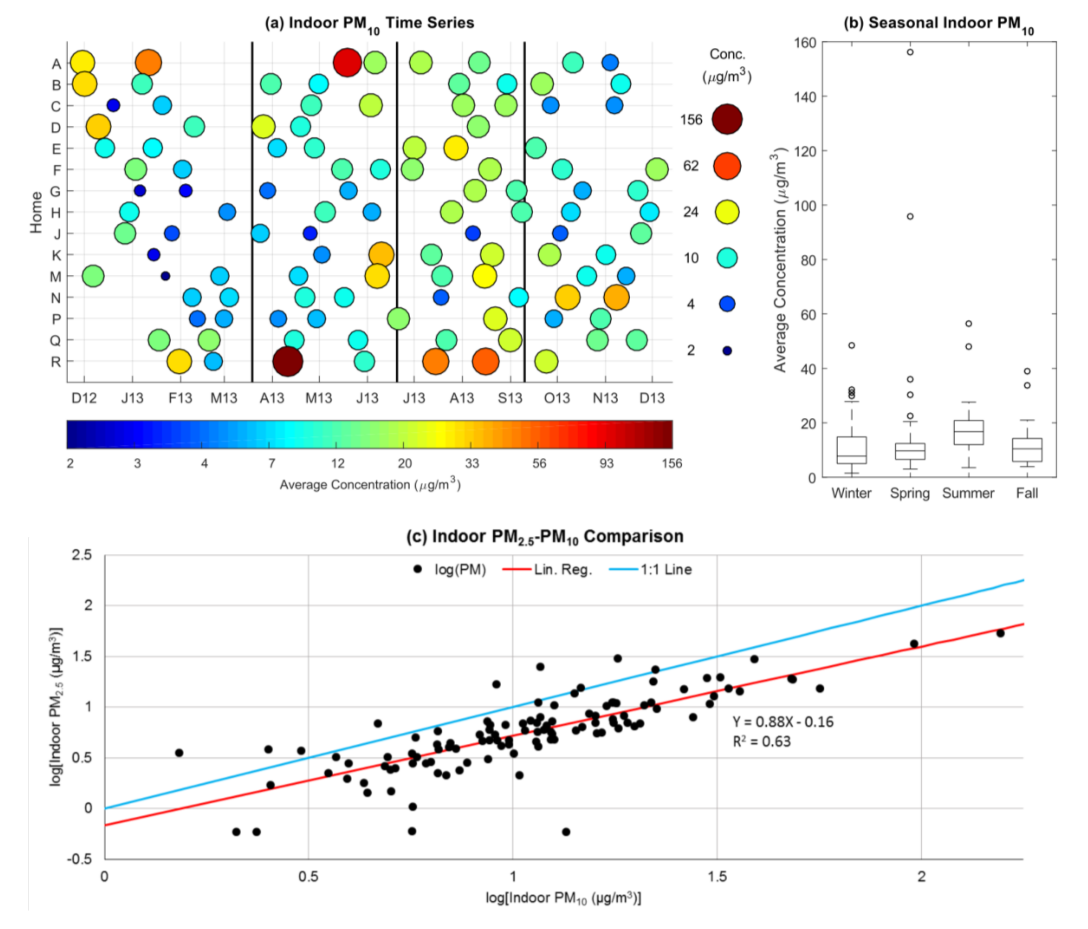
3.1. Indoor and Outdoor Particulate Matter
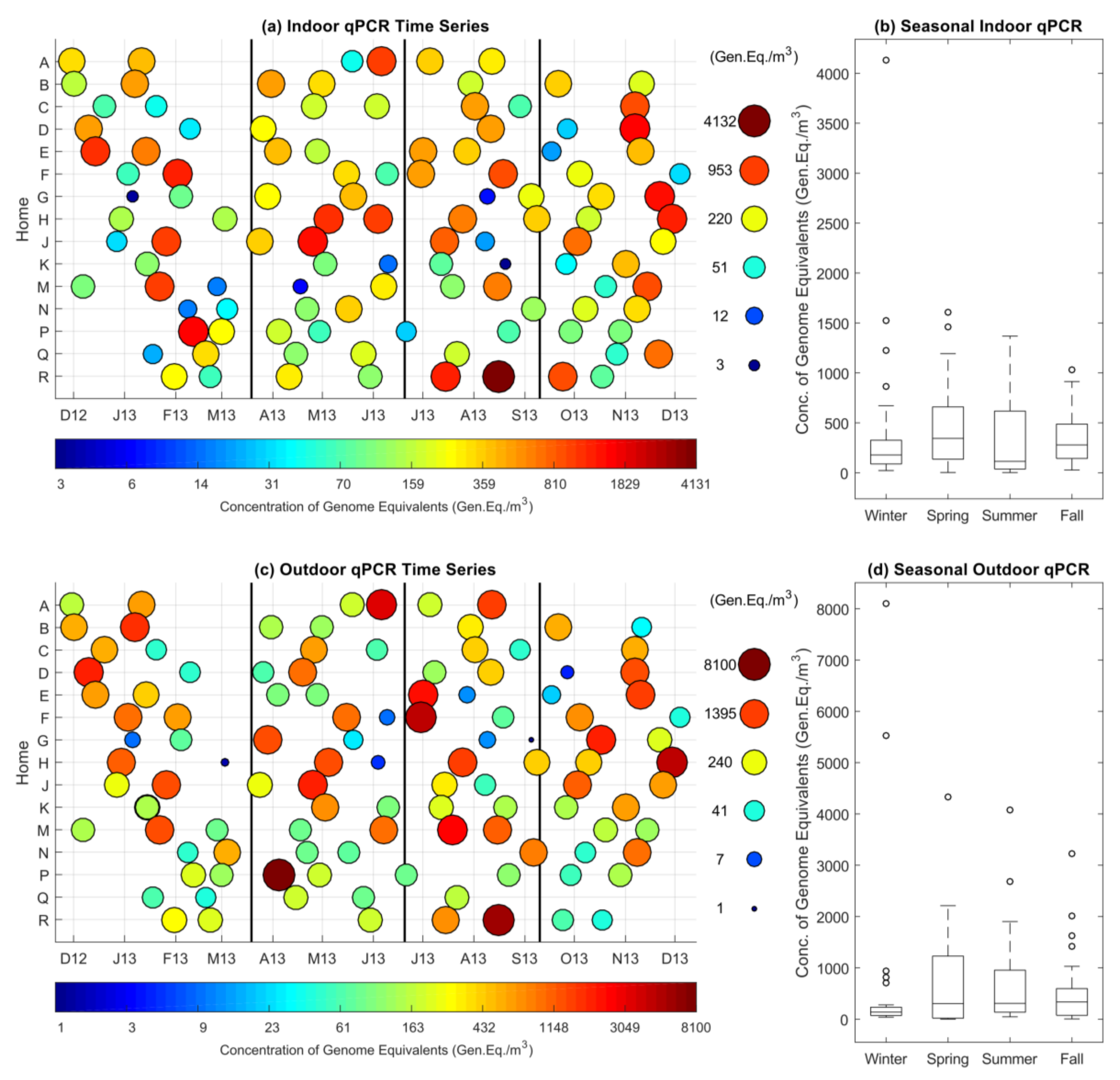
3.2. Indoor and Outdoor qPCR
3.3. Clustering
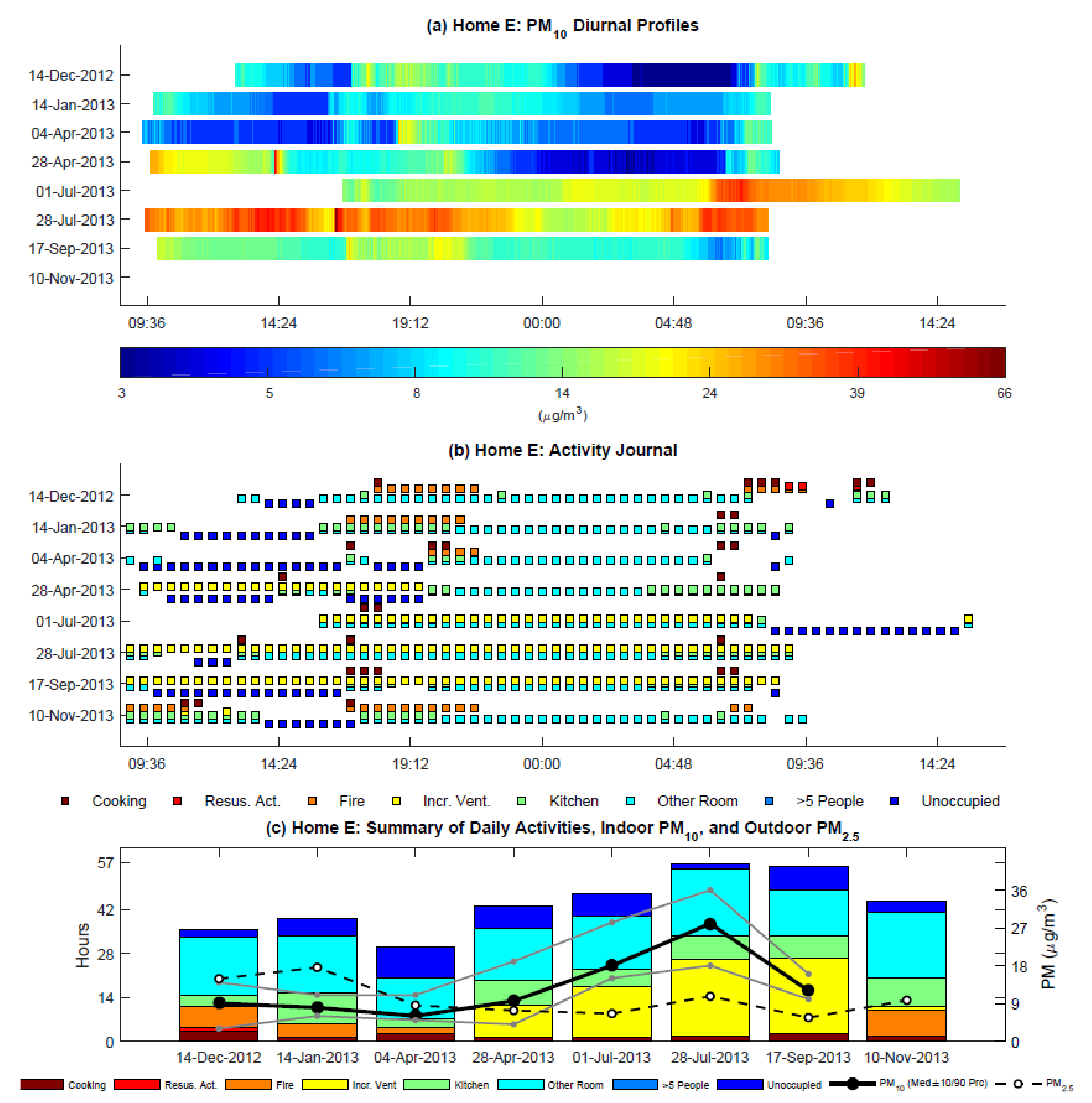
3.4. Activity Journals and Indoor PM10
4. Conclusions
Supplementary Materials
Acknowledgments
Author Contributions
Conflicts of Interest
References
- Dales, R.; Liu, L.; Wheeler, A.J.; Gilbert, N.L. Quality of indoor residential air and health. CMAJ 2008, 179, 147–152. [Google Scholar] [CrossRef] [PubMed]
- Chan, W.R.; Logue, J.M.; Wu, X.; Klepeis, N.E.; Fisk, W.J.; Noris, F.; Singer, B.C. Quantifying fine particle emission events from time-resolved measurements: Method description and application to 18 California low-income apartments. Indoor Air 2018, 28, 89–101. [Google Scholar] [CrossRef] [PubMed]
- Chen, C.; Zhao, B. Review of relationship between indoor and outdoor particles: I/O ratio, infiltration factor and penetration factor. Atmos. Environ. 2011, 45, 275–288. [Google Scholar] [CrossRef]
- Buonanno, G.; Morawska, L.; Stabile, L. Particle emission factors during cooking activities. Atmos. Environ. 2009, 43, 3235–3242. [Google Scholar] [CrossRef]
- Abdullahi, K.; Delgado-Saborit, J.; Harrison, R.M. Emissions and indoor concentrations of particulate matter and its specific chemical components from cooking: A review. Atmos. Environ. 2013, 71, 260–294. [Google Scholar] [CrossRef]
- Jones, N.C.; Thornton, C.A.; Mark, D.; Harrison, R.M. Indoor/outdoor relationships of particulate matter in domestic homes with roadside, urban, and rural locations. Atmos. Environ. 2000, 34, 2603–2612. [Google Scholar] [CrossRef]
- He, C.; Morawska, L.; Hitchins, J.; Gilbert, D. Contribution from indoor sources to particle number and mass concentrations in residential houses. Atmos. Environ. 2004, 38, 3405–3415. [Google Scholar] [CrossRef]
- Olson, D.A.; Burke, J.M. Distributions of PM2.5 Source Strengths for Cooking from the Research Triangle Park Particulate Matter Panel Study. Environ. Sci. Technol. 2006, 40, 163–169. [Google Scholar] [CrossRef] [PubMed]
- Knibbs, L.D.; He, C.; Duchaine, C.; Morawska, L. Vacuum Cleaner Emissions as a Source of Indoor Exposure to Airborne Particles and Bacteria. Environ. Sci. Technol. 2011, 46, 534–542. [Google Scholar] [CrossRef] [PubMed]
- Ferro, A.R.; Kopperud, R.J.; Hildemann, L.M. Source Strengths for Indoor Human Activities that Resuspend Particulate Matter. Environ. Sci. Technol. 2004, 38, 1759–1764. [Google Scholar] [CrossRef] [PubMed]
- Serfozo, N.; Chatoutsidou, S.E.; Lazaridis, M. The effect of particle resuspension during walking activity to PM10 mass and number concentrations in an indoor microenvironment. Build. Environ. 2014, 82, 180–189. [Google Scholar] [CrossRef]
- Larson, T.; Gould, T.; Simpson, C.; Liu, L.-J.S.; Claiborn, C.; Lewtas, J. Source Apportionment of Indoor, Outdoor, and Personal PM2.5 in Seattle, Washington, Using Positive Matrix Factorization. Indoor Air 2004, 54, 1175–1187. [Google Scholar] [CrossRef]
- Bari, Md.A.; Kindzierski, W.B.; Wallace, L.A.; Wheeler, A.J.; MacNeill, M.; Heroux, M.-E. Indoor and Outdoor Levels and Sources of Submicron Particles (PM1) at Homes in Edmonton, Canada. Environ. Sci. Technol. 2015, 49, 6419–6429. [Google Scholar] [CrossRef] [PubMed]
- Perrino, C.; Tofful, L.; Canepari, S. Chemical characterization of indoor and outdoor fine particulate matter in an occupied apartment in Rome, Italy. Indoor Air 2015. [Google Scholar] [CrossRef] [PubMed]
- Lim, M.T.; Phan, A.; Roddy, D.; Harvey, A. Technologies for measurement and mitigation of particulate emissions from domestic combustion of biomass: A review. Renew. Sustain. Energy Rev. 2015, 49, 574–584. [Google Scholar] [CrossRef]
- Urso, P.; Cattaneo, A.; Garramone, G.; Peruzzo, C.; Cavallo, D.M.; Carrer, P. Identification of particulate matter determinants in residential homes. Build. Environ. 2015, 86, 61–69. [Google Scholar] [CrossRef]
- Meng, Q.Y.; Spector, D.; Colome, S.; Turpin, B. Determinants of indoor and personal exposure to PM2.5 of indoor and outdoor origin during the RIOPA study. Atmos. Environ. 2009, 43, 5750–5758. [Google Scholar] [CrossRef] [PubMed]
- Klepeis, N.E.; Bellettiere, J.; Hughes, S.C.; Nguyen, B.; Berardi, V.; Liles, S.; Obayashi, S.; Hofstetter, C.R.; Blumberg, E.; Hovell, M.F. Fine particles in homes of predominantly low-income families with children and smokers: Key physical and behavioral determinants to inform indoor-air-quality interventions. PLoS ONE 2017, 12, e0177718. [Google Scholar] [CrossRef] [PubMed]
- Richardson, G.; Eick, S.A.; Shaw, S.R. Designing a Simple Tool Kit and Protocol for the Investigation of the Indoor Environment in Homes. Indoor Built Environ. 2006, 15, 411–424. [Google Scholar] [CrossRef]
- Ramachandran, G.; Adgate, J.L.; Pratt, G.C.; Sexton, K. Characterizing Indoor and Outdoor 15 Minute Average PM2.5 Concentrations in Urban Neighborhoods. Aerosol Sci. Technol. 2003, 37, 33–45. [Google Scholar] [CrossRef]
- Williams, R.; Suggs, J.; Rea, A.; Leovic, K.; Vette, A.; Croghan, C.; Sheldon, L.; Rodes, C.; Thornburg, J.; Ejire, A.; et al. The Research Triangle Park particulate matter panel study: PM mass concentration relationships. Atmos. Environ. 2003, 37, 5349–5364. [Google Scholar] [CrossRef]
- Jaenicke, R. Abundance of Cellular Material and Proteins in the Atmosphere. Science 2005, 308, 73. [Google Scholar] [CrossRef] [PubMed]
- Adams, R.I.; Miletto, M.; Lindow, S.E.; Taylor, J.W.; Bruns, T.D. Airborne Bacterial Communities in Residences: Similarities and Differences with Fungi. PLoS ONE 2014, 9, e91283. [Google Scholar] [CrossRef] [PubMed]
- Qian, J.; Hospodsky, D.; Yamamoto, N.; Nazaroff, W.W.; Peccia, J. Size-resolved emission rates of airborne bacteria and fungi in an occupied classroom. Indoor Air 2012, 22, 339–351. [Google Scholar] [CrossRef] [PubMed]
- Burge, H. Bioaerosols: Prevalence and health effects in the indoor environment. J. Allergy Clin. Immunol. 1990, 86, 687–701. [Google Scholar] [CrossRef]
- Hospodsky, D.; Qian, J.; Nazaroff, W.W.; Yamamoto, N.; Bibby, K.; Rismani-Yazdi, H.; Peccia, J. Human Occupancy as a Source of Indoor Airborne Bacteria. PLoS ONE 2012, 7, e34867. [Google Scholar] [CrossRef] [PubMed]
- Torvinen, E.; Torkko, P.; Rintala, A.N.H. Real-time PCR detection of environmental mycobacteria in house dust. J. Microbiol. Methods 2010, 82, 78–84. [Google Scholar] [CrossRef] [PubMed]
- Kaarakainen, P.; Meklin, T.; Hyvärinen, A.; Kärkkäinen, P.; Vepsäläinen, A.; Hirvonen, M.-R.; Nevalainen, A. Seasonal variation in airborne microbial concentrations and diversity at landfill, urban and rural sites. CLEAN–Soil Air Water 2008, 36, 556–563. [Google Scholar] [CrossRef]
- Kahle, D.; Wickham, H. ggmap: Spatial Visualization with ggplot2. R J. 2013, 5, 144–161. [Google Scholar]
- Barberán, A.; Dunn, R.R.; Reich, B.J.; Pacifici, K.; Laber, E.B.; Menninger, H.L.; Morton, J.M.; Henley, J.B.; Leff, J.W.; Miller, S.L.; et al. The ecology of microscopic life in household dust. Proc. R. Soc. B 2015, 282, 20151139. [Google Scholar] [CrossRef] [PubMed]
- Dutton, S.J.; Schauer, J.J.; Vedal, S.; Hannigan, M.P. PM 2.5 characterization for time series studies: Pointwise uncertainty estimation and bulk speciation methods applied in Denver. Atmos. Environ. 2009, 43, 1136–1146. [Google Scholar] [CrossRef] [PubMed]
- Emerson, J.B.; Keady, P.B.; Brewer, T.E.; Clements, N.; Morgan, E.E.; Awerbuch, J.; Miller, S.L.; Fierer, N. Impacts of Flood Damage on Airborne Bacteria and Fungi in Homes after the 2013 Colorado Front Range Flood. Environ. Sci. Technol. 2015, 49, 2675–2684. [Google Scholar] [CrossRef] [PubMed]
- Emerson, J.B.; Keady, P.B.; Clements, N.; Morgan, E.E.; Awerbuch, J.; Miller, S.L.; Fierer, N. High temporal variability in airborne bacterial diversity and abundance inside single-family residences. Indoor Air 2017, 27, 576–586. [Google Scholar] [CrossRef] [PubMed]
- McNamara, M.L.; Noonan, C.W.; Ward, T.J. Correction factor for continuous monitoring of wood smoke fine particulate matter. Aerosol Air Qual. Res. 2011, 11, 315–322. [Google Scholar] [CrossRef] [PubMed]
- Spinazzè, A.; Fanti, G.; Borghi, F.; Del Buono, L.; Campagnolo, D.; Rovelli, S.; Cattaneo, A.; Cavallo, D.M. Field comparison of instruments for exposure assessment of airborne ultrafine particles and particulate matter. Atmos. Environ. 2017, 154, 274–284. [Google Scholar] [CrossRef]
- Rivas, I.; Mazaheri, M.; Viana, M.; Moreno, T.; Clifford, S.; He, C.; Bischof, O.F.; Martins, V.; Reche, C.; Alastuey, A.; et al. Identification of technical problems affecting performance of DustTrak DRX aerosol monitors. Sci. Total Environ. 2017, 584, 849–855. [Google Scholar] [CrossRef] [PubMed]
- Litt, J.S.; Goss, C.; Diao, L.; Allshouse, A.; Diaz-Castillo, S.; Barwell, R.A.; Hendrikson, E.; Miller, S.L.; DiGuiseppi, C. Housing Environments and Child Health Conditions Among Recent Mexican Immigrant Families: A Population-Based Study. J. Immigr. Minor. Health 2010, 12, 617–625. [Google Scholar] [CrossRef] [PubMed]
- Hancock, E.; Norton, P.; Hendron, B. Building America System Performance Test Practices: Part 2, Air-Exchange Measurements; NREL/TP-550-30270; National Renewable Energy Laboratory: Golden, CO, USA, 2002; p. 2. [Google Scholar]
- IECC. International Energy Conservation Code. Building Technologies Program Air Leakage Guide, Report PNNL-SA-82900. 2012. Available online: https://www.energycodes.gov/sites/default/files/documents/BECP_Buidling%20Energy%20Code%20Resource%20Guide%20Air%20Leakage%20Guide_Sept2011_v00_lores.pdf (accessed on 10 January 2018).
- Ott, W.; Wallace, L.; Mage, D. Predicting particulate (PM10) personal exposure distributions using a random component superposition statistical model. Air Waste Manag. Assoc. 2000, 50, 1390–1406. [Google Scholar] [CrossRef]
- Wallace, L.A.; Mitchell, H.; O’Connor, G.T.; Neas, L.; Lippmann, M.; Kattan, M.; Koenig, J.; Stout, J.W.; Vaughn, B.J.; Wallace, D.; et al. Particle concentrations in inner-city homes of children with asthma: The effect of smoking, cooking, and outdoor pollution. Environ. Health Perspect. 2003, 111, 1265–1272. [Google Scholar] [CrossRef] [PubMed]
- Wallace, W.; Williams, R. Use of personal-indoor-outdoor sulfur concentrations to estimate the infiltration factor and outdoor exposure factor for individual homes and persons. Environ. Sci. Technol. 2005, 39, 1707–1714. [Google Scholar] [CrossRef] [PubMed]
- Miller, S.L.; Scaramella, P.; Campe, J.; Goss, C.W.; Diaz-Castillo, S.; Hendrikson, E.; DiGuiseppi, C.; Litt, J. An assessment of indoor air quality in recent Mexican immigrant housing in Commerce City, Colorado. Atmos. Environ. 2009, 43, 5661–5667. [Google Scholar] [CrossRef]
- Yanosky, J.D.; Williams, P.L.; MacIntosh, D.L. A comparison of two direct-reading aerosol monitors with the federal reference method for PM2.5 in indoor air. Atmos. Environ. 2002, 36, 107–113. [Google Scholar] [CrossRef]
- Kim, J.Y.; Magari, S.R.; Herrick, R.F.; Smith, T.J.; Christiani, D.C. Comparison of Fine Particle Measurements from a Direct-Reading Instrument and a Gravimetric Sampling Method. J. Occup. Environ. Hyg. 2004, 1, 707–715. [Google Scholar] [CrossRef] [PubMed]
- Moya, M.; Madronich, S.; Retama, A.; Weber, R.; Baumann, K.; Nenes, A.; Castillejos, M.; Ponce de Leon, C. Identification of chemistry-dependent artifacts on gravimetric PM fine readings at the T1 site during the MILAGRO field campaign. Atmos. Environ. 2011, 45, 244–252. [Google Scholar] [CrossRef]
- Klepeis, N.E.; Hughes, S.C.; Edwards, R.D.; Allen, T.; Johnson, M.; Chowdhury, Z.; Smith, K.R.; Boman-Davis, M.; Bellettiere, J.; Hovell, M.F. Promoting smoke-free homes: A novel behavioral intervention using real-time audio-visual feedback on airborne particle levels. PLoS ONE 2013, 8, e73251. [Google Scholar] [CrossRef] [PubMed]
- ASHRAE 169-2006. Standard for Weather Data for Building Design Standards Created by American Society of Heating, Refrigerating and Air-Conditioning Engineers; ASHRAE: Atlanta, GA, USA; Available online: https://www.ashrae.org/resources--publications/bookstore/climate-data-center#std169 (accessed on 10 January 2018).


| Home | Location | Year Built | Time in Home (Years) | Surface Area (m2) | Volume (m3) | Basement/Garage | # Residents | # Kids | #Male | # Female |
|---|---|---|---|---|---|---|---|---|---|---|
| A | Boulder city 1 | 1965 | 2–5 | 167.4 | 333.9 | Yes/Yes | 3 | 1 | 1 | 2 |
| B | Fort Collins 1 | 1995 | 6–10 | 347.2 | 1011.1 | Yes/Yes | 3 | 1 | 1 | 2 |
| C | Boulder city 1 | 1999 | 6–10 | 318.5 | 885.1 | Yes/Yes | 4 | 2 | 2 | 2 |
| D | Lyons 1 | 1970 | 6–10 | 129.9 | 326.5 | No/Yes | 3 | 1 | 1 | 2 |
| E | Fort Collins 1 | 1965 | 6–10 | 278.1 | 663.4 | Yes/Yes | 4 | 2 | 2 | 2 |
| F | Boulder city 1 | 1985 | 6–10 | 279.6 | 765.4 | Yes/Yes | 3 to 5 | 1 to 3 | 1 to 2 | 2 to 3 |
| G | Boulder city 1 | 1986 | 11–20 | 465.7 | 1208.2 | Yes/Yes | 2 | 0 | 1 | 1 |
| H | Boulder mountain 2 | 1985 | >20 | 114.5 | 276.5 | No/No | 2 | 0 | 1 | 1 |
| J | Boulder city 1 | 1968 | >20 | 229 | 517.7 | Yes/Yes | 3 | 0 | 2 | 1 |
| K | Boulder city 1 | 1968 | >20 | 219.8 | 611.7 | Yes/Yes | 2 | 0 | 1 | 1 |
| M | Boulder mountain 2 | 1970 | >20 | 195.1 | 581.5 | No/No | 3 | 0 | 1 | 2 |
| N | Boulder city 1 | 1973 | 2–5 | 230.6 | 530.1 | Yes/Yes | 4 | 2 | 2 | 2 |
| P | Niwot 2 | 1977 | 11–20 | 372.5 | 930.3 | Yes/Yes | 2 | 0 | 1 | 1 |
| Q | Longmont 1 | 1960 | 2–5 | 131 | 299.5 | Yes/Yes | 3 | 0 | 1 | 2 |
| R | Boulder city 1 | 2006 | 6–10 | 255.2 | 759.6 | Yes/No | 4 | 2 | 1 | 3 |
| Home | Cook Stove | Heating | Fireplace | Ventilation/Heating Type | Air-Conditioning (AC) | Filter 1 | VPS 2 | ACH50 3 |
|---|---|---|---|---|---|---|---|---|
| A | Gas | Gas | Wood | Forced Air | None/Evaporative | MERV 4 | 6 | 11.8 |
| B | Electric | Gas | Gas | Forced Air | Central | MERV 4 | 3 | 4.4 |
| C | Gas | Gas | Gas | Forced Air | Central | MERV 8 | 5 | 5.0 |
| D | Gas | Gas | Wood | Radiator, Baseboard, or Space Heater | None | No | 5 | 16.4 |
| E | Gas | Gas | Gas | Forced Air | Central | MERV 8 | 3 | 5.9 |
| F | Gas | Gas | Wood | Forced Air | Evaporative | MERV 4 | 5 | 8.8 |
| G | Gas | Gas | Wood | Forced Air | Central | Electrostatic, MERV 12 | 5 | 6.8 |
| H | Electric | Wood | Wood | Wood-burning or pellet stove/Fireplace | None | No | 5 | 9.6 |
| J | Electric | Gas | Wood | Forced Air | Central | Electrostatic, MERV 12 | 3 | 8.9 |
| K | Electric | Gas | Wood | Forced Air | None | Electrostatic, MERV 12 | 3 | 9.0 |
| M | Gas | Gas/Wood | Wood | Wood-burning or pellet Stove/Fireplace | None | No | 5 | 7.0 |
| N | Gas | Gas | Gas | Forced Air | Central | Electrostatic, MERV 12 | 4 | 5.6 |
| P | Gas | Gas | None | Forced Air | Central | MERV 4 | 6 | 6.3 |
| Q | Electric | Gas | None | Radiator, Baseboard, or Space Heater | Window AC Unit(s) | No | 4 | 15.6 |
| R | Gas | None | Gas | None/Radiant Heat | Evaporative | No | 5 | 4.2 |
© 2018 by the authors. Licensee MDPI, Basel, Switzerland. This article is an open access article distributed under the terms and conditions of the Creative Commons Attribution (CC BY) license (http://creativecommons.org/licenses/by/4.0/).
Share and Cite
Clements, N.; Keady, P.; Emerson, J.B.; Fierer, N.; Miller, S.L. Seasonal Variability of Airborne Particulate Matter and Bacterial Concentrations in Colorado Homes. Atmosphere 2018, 9, 133. https://doi.org/10.3390/atmos9040133
Clements N, Keady P, Emerson JB, Fierer N, Miller SL. Seasonal Variability of Airborne Particulate Matter and Bacterial Concentrations in Colorado Homes. Atmosphere. 2018; 9(4):133. https://doi.org/10.3390/atmos9040133
Chicago/Turabian StyleClements, Nicholas, Patricia Keady, Joanne B. Emerson, Noah Fierer, and Shelly L. Miller. 2018. "Seasonal Variability of Airborne Particulate Matter and Bacterial Concentrations in Colorado Homes" Atmosphere 9, no. 4: 133. https://doi.org/10.3390/atmos9040133
APA StyleClements, N., Keady, P., Emerson, J. B., Fierer, N., & Miller, S. L. (2018). Seasonal Variability of Airborne Particulate Matter and Bacterial Concentrations in Colorado Homes. Atmosphere, 9(4), 133. https://doi.org/10.3390/atmos9040133