Numerical Simulation of Heavy Rainfall in August 2014 over Japan and Analysis of Its Sensitivity to Sea Surface Temperature


Abstract
1. Introduction
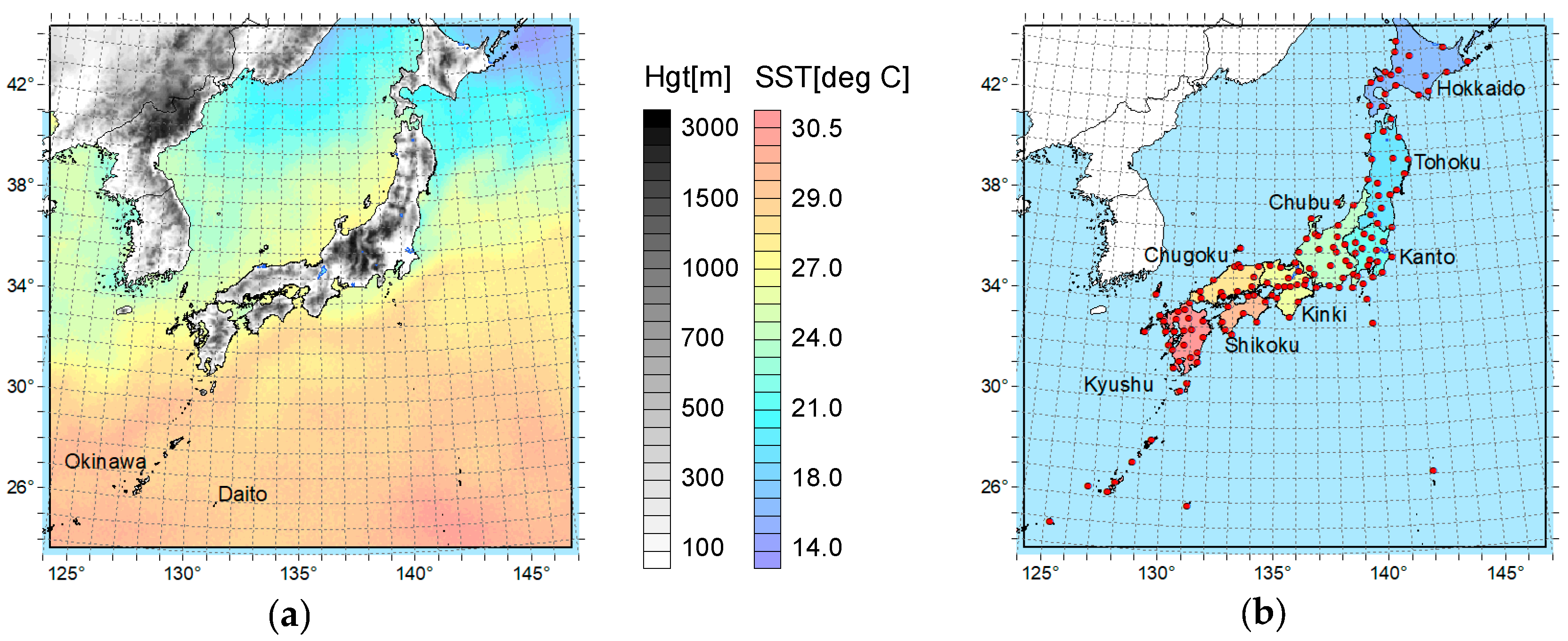
2. Methods
2.1. Common WRF Configurations
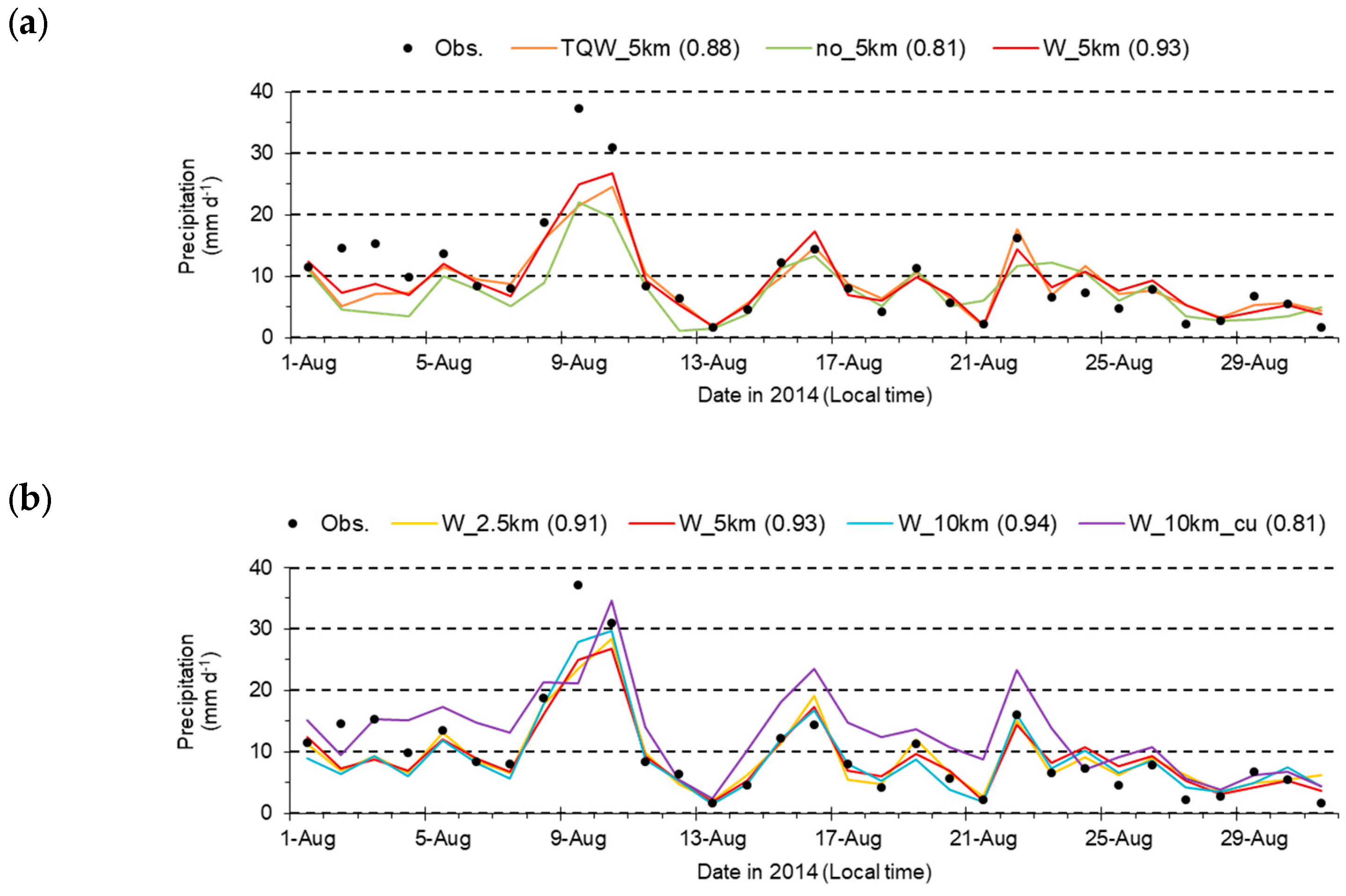
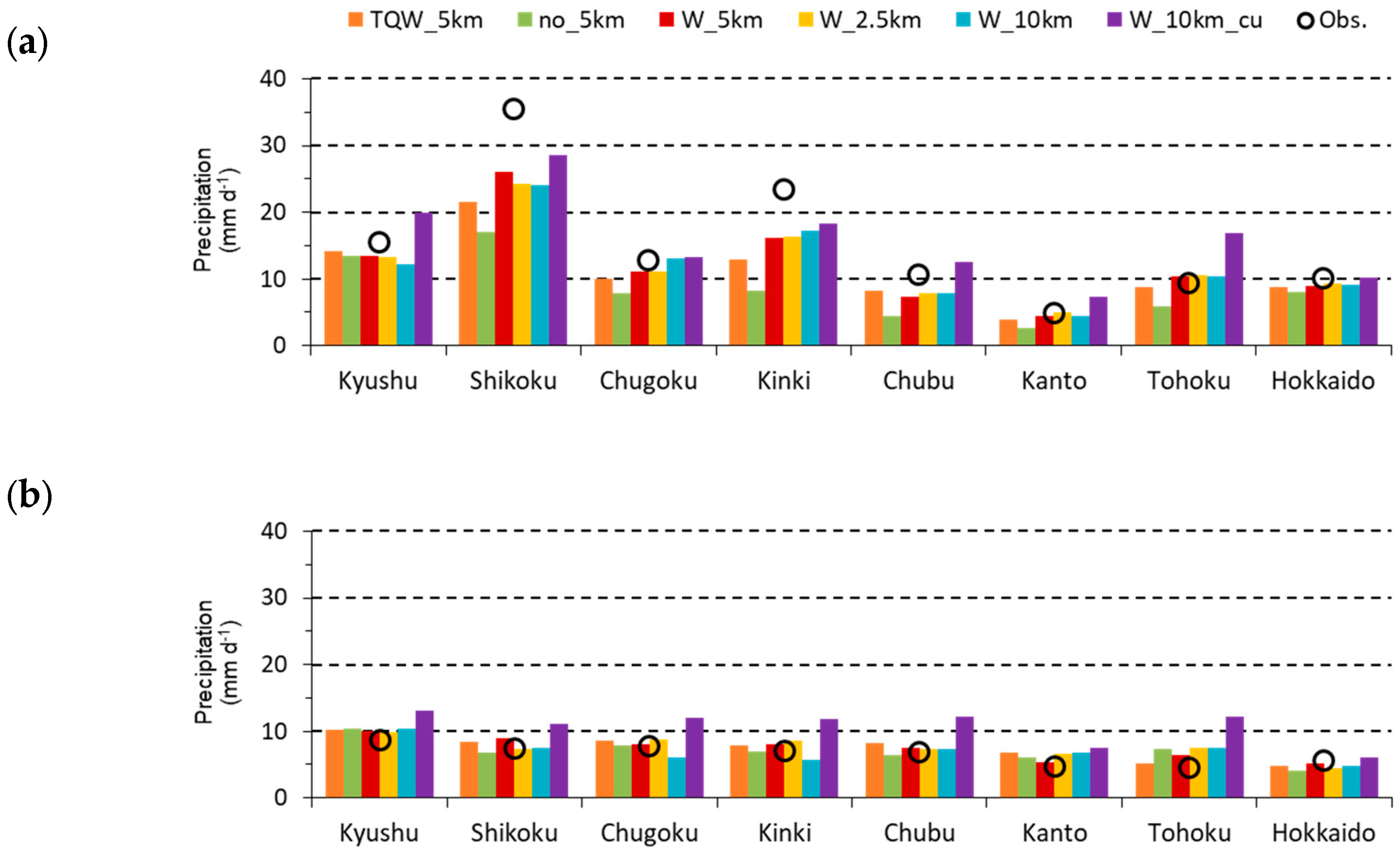
2.2. Selection of Optimal WRF Setting
2.3. Sensitivity Analysis on SST
3. Results and Discussion
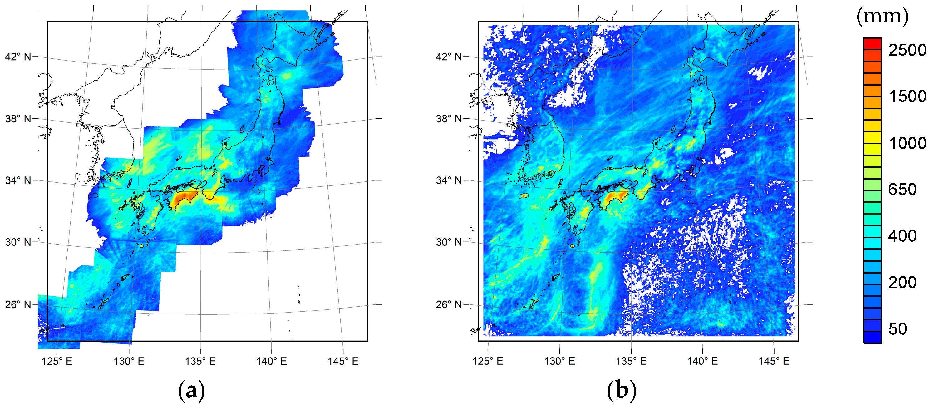
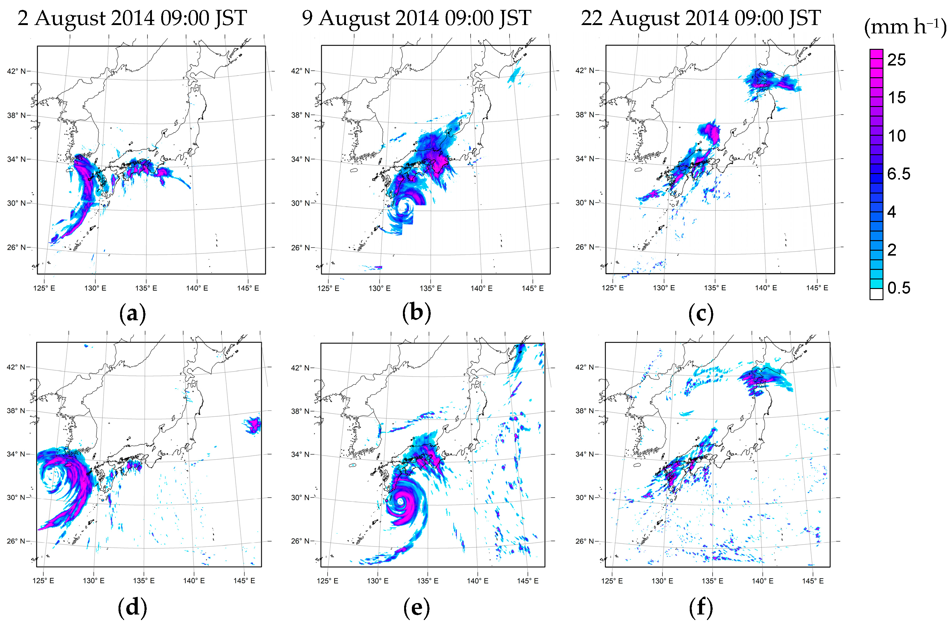
3.1. Reproducibility of the Heavy Rainfall
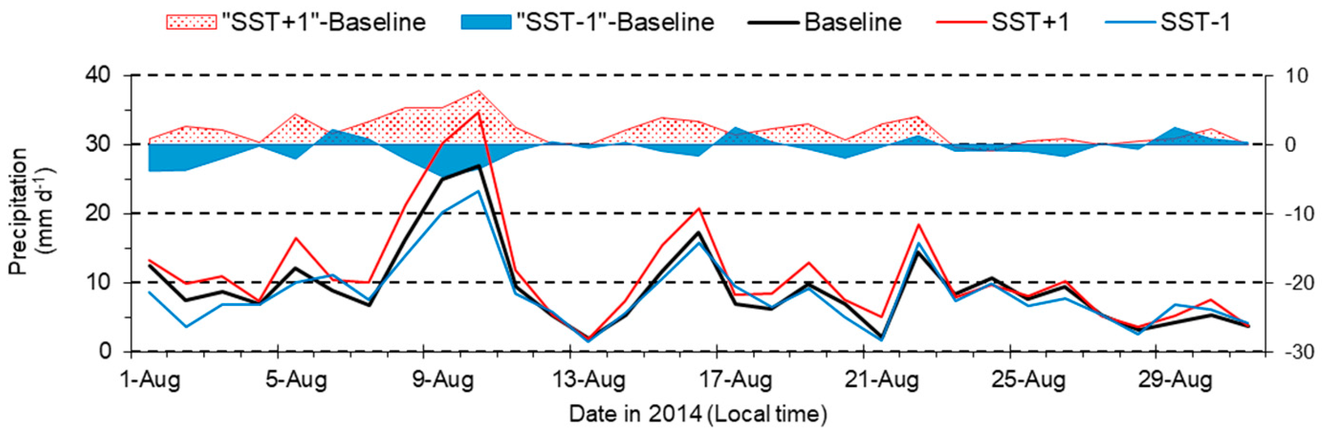
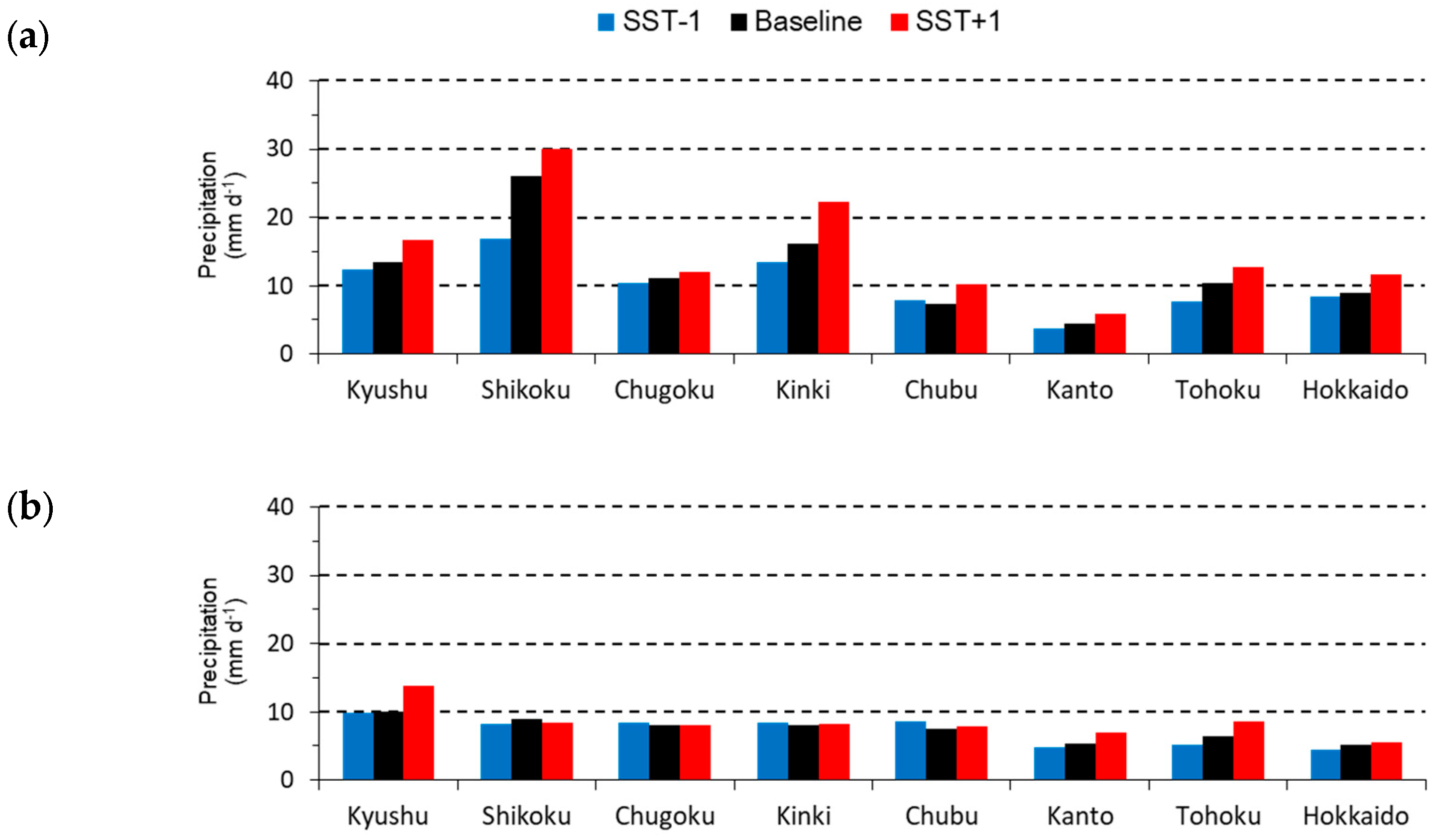
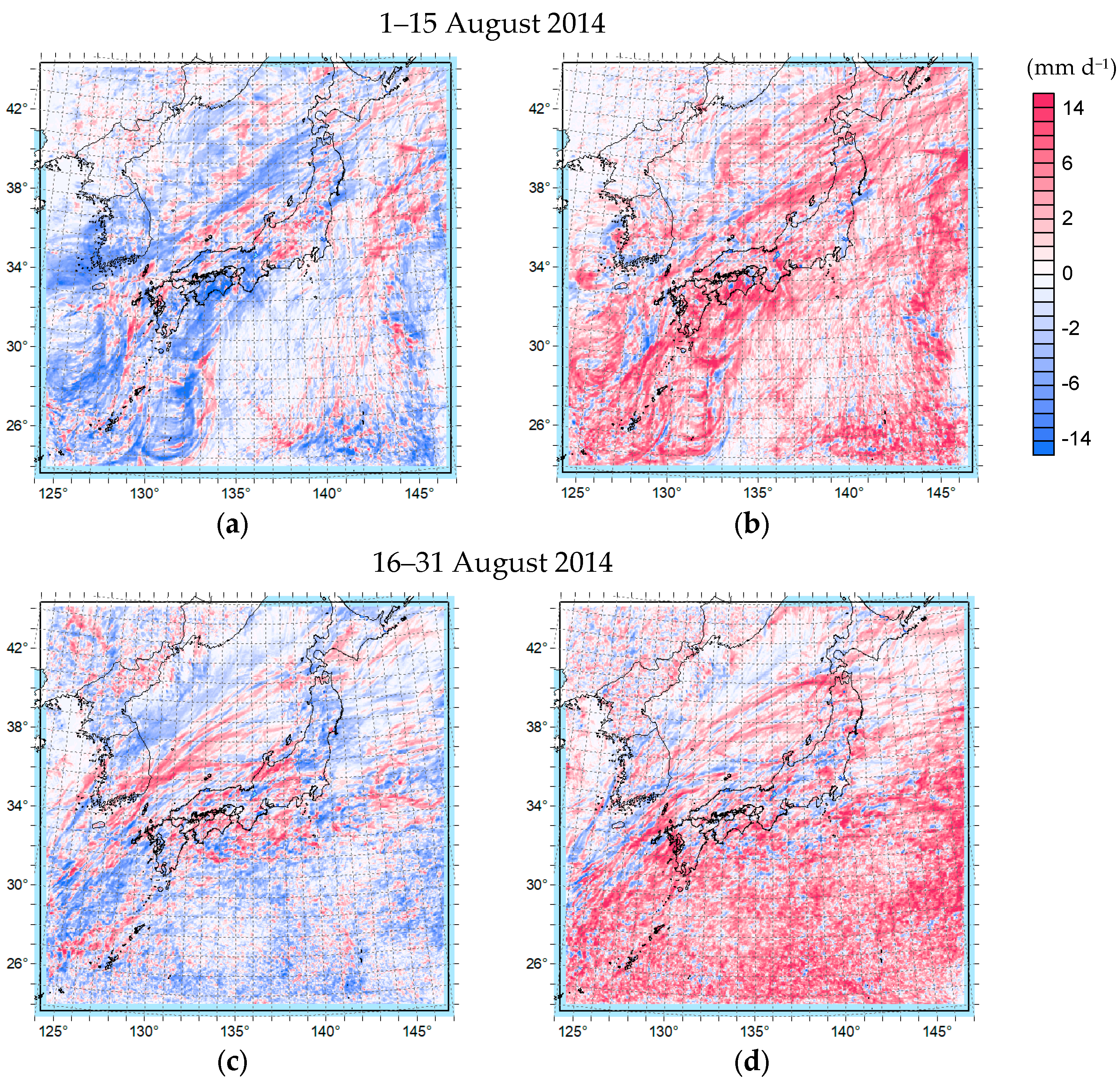
3.2. Sensitivity of Precipitation to SST
4. Conclusions
Acknowledgments
Author Contributions
Conflicts of Interest
References
- Intergovernmental Panel on Climate Change. CLIMATE CHANGE 2014 Synthesis Report; Intergovernmental Panel on Climate Change: Geneva, Switzerland, 2014. [Google Scholar]
- Boer, G.J. Climate change and the regulation of the surface moisture and energy budgets. Clim. Dyn. 1993, 8, 225–239. [Google Scholar] [CrossRef]
- Allen, M.R.; Ingram, W.J. Constraints on the future changes in climate and the hydrological cycle. Nature 2002, 419, 224–232. [Google Scholar] [CrossRef] [PubMed]
- Trenberth, K.E.; Dai, A.; Rasmussen, R.M.; Parsons, D.B. The changing character of precipitation. Bull. Am. Meteorol. Soc. 2003, 84, 1205–1217. [Google Scholar] [CrossRef]
- Pall, P.; Allen, M.R.; Stone, D.A. Testing the Clausius–Clapeyron constraint on changes in extreme precipitation under CO2 warming. Clim. Dyn. 2007, 28, 351–363. [Google Scholar] [CrossRef]
- Lenderink, G.; van Meijgaard, E. Increase in hourly precipitation extremes beyond expectations from temperature changes. Nat. Geosci. 2008, 1, 511–514. [Google Scholar] [CrossRef]
- Nayak, S.; Dairaku, K. Future changes in extreme precipitation intensities associated with temperature under SRES A1B scenario. Hydrol. Res. Lett. 2016, 10, 139–144. [Google Scholar] [CrossRef][Green Version]
- Japan Meteorological Agency. Global Warming Projection Vol. 7; Japan Meteorological Agency: Chiyoda-ku, Japan, 2008. (In Japanese)
- Fujibe, F. Relationship between Interannual Variations of Extreme Hourly Precipitation and Air/Sea-Surface Temperature in Japan. SOLA 2015, 11, 5–9. [Google Scholar] [CrossRef]
- Cruz, F.T.; Narisma, G.T. WRF simulation of the heavy rainfall over Metropolitan Manila, Philippines during tropical cyclone Ketsana: A sensitivity study. Meteorol. Atmos. Phys. 2016, 128, 415–428. [Google Scholar] [CrossRef]
- Ishikawa, H.; Oku, Y.; Kim, S.; Takemi, T.; Yoshino, J. Estimation of a possible maximum flood event in the Tone River basin, Japan caused by a tropical cyclone. Hydrol. Processes 2013, 27, 3292–3300. [Google Scholar] [CrossRef]
- Nakamura, R.; Shibayama, T.; Esteban, M.; Iwamoto, T. Future typhoon and storm surges under different global warming scenarios: Case study of typhoon Haiyan (2013). Nat. Hazards 2016, 82, 1645–1681. [Google Scholar] [CrossRef]
- Yoshida, K.; Sugi, M.; Mizuta, R.; Murakami, H.; Ishii, M. Future Changes in Tropical Cyclone Activity in High-Resolution Large-Ensemble Simulations. Geophys. Res. Lett. 2017, 44, 9910–9917. [Google Scholar] [CrossRef]
- Brayshaw, D.J.; Hoskins, B.; Blackburn, M. The Basic Ingredients of the North Atlantic Storm Track. Part II: Sea Surface Temperature. J. Atmos. Sci. 2011, 68, 1784–1805. [Google Scholar] [CrossRef]
- Sugi, M.; Noda, A.; Sato, N. Influence of the Global Warming on Tropical Cyclone Climatology: An Experiment with the JMA Global Model. J. Meteorol. Soc. Japan 2002, 80, 249–272. [Google Scholar] [CrossRef]
- Knutson, T.R.; McBride, J.L.; Chan, J.; Emanuel, K.; Holland, G.; Landsea, C.; Held, I.; Kossin, J.P.; Srivastava, A.K.; Sugi, M. Tropical cyclones and climate change. Nat. Geosci. 2010, 3, 157–163. [Google Scholar] [CrossRef]
- Yamada, Y.; Satoh, M.; Sugi, M.; Kodama, C.; Noda, A.T.; Nakano, M.; Nasuno, T. Response of Tropical Cyclone Activity and Structure to Global Warming in a High-Resolution Global Nonhydrostatic Model. J. Clim. 2017, 30, 9703–9724. [Google Scholar] [CrossRef]
- Kanada, S.; Takemi, T.; Kato, M.; Yamasaki, S.; Fudeyasu, H.; Tsuboki, K.; Arakawa, O.; Takayabu, I. A Multimodel Intercomparison of an Intense Typhoon in Future, Warmer Climates by Four 5-km-Mesh Models. J. Clim. 2017, 30, 6017–6036. [Google Scholar] [CrossRef]
- Takayabu, I.; Hibino, K.; Sasaki, H.; Shiogama, H.; Mori, N.; Shibutani, Y.; Takemi, T. Climate change effects on the worst-case storm surge: A case study of Typhoon Haiyan. Environ. Res. Lett. 2015, 10, 064011. [Google Scholar] [CrossRef]
- Lackmann, G.M. Hurricane Sandy before 1900 and after 2100. Bull. Am. Meteorol. Soc. 2015, 96, 547–560. [Google Scholar] [CrossRef]
- Volosciuk, C.; Maraun, D.; Semenov, V.A.; Tilinia, N.; Gulev, S.K.; Latif, M. Rising Mediterranean Sea Surface Temperatures Amplify Extreme Summer Precipitation in Central Europe. Sci. Rep. 2016, 6, 32450. [Google Scholar] [CrossRef] [PubMed]
- Manda, A.; Nakamura, H.; Iizuka, S.; Miyama, T.; Moteki, Q.; Yoshioka, M.K.; Nishii, K.; Miyasaka, T. Impacts of a warming marginal sea on torrential rainfall organized under the Asian summer monsoon. Sci. Rep. 2014, 4, 5741. [Google Scholar] [CrossRef] [PubMed]
- Lee, D.K.; Cha, D.H.; Kang, H.S. Regional climate simulation of the 1998 summer flood over East Asia. J. Meteorol. Soc. Japan 2004, 82, 1735–1753. [Google Scholar] [CrossRef]
- Lyra, A.; Tavares, P.; Chou, S.C.; Sueiro, G.; Dereczynski, C.; Sondermann, M.; Silva, A.; Marengo, J.; Giarolla, A. Climate change projections over three metropolitan regions in Southeast Brazil using the non-hydrostatic Eta regional climate model at 5-km resolution. Theor. Appl. Climatol. 2017, 1–20. [Google Scholar] [CrossRef]
- Zhang, X.; Zwiers, F.W.; Li, G.; Wan, H.; Cannon, A.J. Complexity in estimating past and future extreme short-duration rainfall. Nat. Geosci. 2017, 10, 255–259. [Google Scholar] [CrossRef]
- Skamarock, W.C.; Klemp, J.B.; Dudhia, J.; Gill, D.O.; Baker, D.M.; Duda, M.G.; Huang, X.-Y.; Wang, W.; Powers, J.G. A Description of the Advanced Research WRF Version 3; Technical Note TN-475+STR; NCAR: Boulder, CO, USA, 2008. [Google Scholar]
- Ting, M.; Wang, H. Summertime U.S. Precipitation Variability and Its Relation to Pacific Sea Surface Temperature. J. Clim. 1997, 10, 1853–1873. [Google Scholar] [CrossRef]
- Yamamoto, M.; Hirose, N. Influence of assimilated SST on regional atmospheric simulation: A case of a cold-air outbreak over the Japan Sea. Atmos. Res. 2008, 9, 13–17. [Google Scholar] [CrossRef]
- Iizuka, S. Simulations of wintertime precipitation in the vicinity of Japan: Sensitivity to fine-scale distributions of sea surface temperature. J. Geophys. Res. 2010, 115, D10107. [Google Scholar] [CrossRef]
- Pepler, A.S.; Alexander, L.V.; Evans, J.P.; Sherwood, S.C. The influence of local sea surface temperatures on Australian east coast cyclones. J. Geophys. Res. Atmos. 2016, 121, 352–363. [Google Scholar] [CrossRef]
- Takahashi, H.; Ishizaki, N.; Kawase, H.; Hara, M.; Yoshikane, T.; Ma, X.; Kimura, F. Potential Impact of Sea Surface Temperature on Winter Precipitation over the Japan Sea Side of Japan: A Regional Climate Modeling Study. J. Meteorol. Soc. Japan 2013, 91, 471–488. [Google Scholar] [CrossRef]
- Reynolds, W.R.; Folland, C.K.; Parker, D.E. Biases in satellite-derived sea-surface-temperature data. Nature 1989, 341, 728–731. [Google Scholar] [CrossRef]
- Reynolds, W.R. Impact of Mount Pinatubo aerosols on satellite-derived sea surface temperatures. J. Clim. 1993, 6, 768–774. [Google Scholar] [CrossRef]
- Chan, P.-K.; Gao, B.-C. A comparison of MODIS, NCEP, and TMI sea surface temperature datasets. IEEE Geosci. Remote Sens. Lett. 2005, 2, 270–274. [Google Scholar] [CrossRef]
- Reynolds, W.R.; Chelton, D.B. Comparisons of daily sea surface temperature analyses for 2007–2008. J. Clim. 2010, 23, 3545–3562. [Google Scholar] [CrossRef]
- Fu, H.; Wang, Y. Effect of uncertainties in sea surface temperature dataset on the simulation of typhoon Nangka (2015). Atmos. Sci. Lett. 2017. [Google Scholar] [CrossRef]
- Qingyuan, W.; Yanan, W.; Yiwei, L. Comparison of two Centennial-scale Sea Surface Temperature Datasets in the Regional Climate Change Studies of the China Seas. IOP Conf. Ser. Earth Environ. Sci. 2017, 81, 012077. [Google Scholar] [CrossRef]
- Japan Meteorological Agency. Prompt Report on Heavy Precipitation in August 2014; Japan Meteorological Agency: Chiyoda-ku, Japan, 2014. (In Japanese)
- Japan Meteorological Agency. Available online: http://www.data.jma.go.jp/kaiyou/shindan/index.html (accessed on 20 December 2017).
- Shimadera, H.; Kondo, A.; Shrestha, K.L.; Kitaoka, K.; Inoue, Y. Numerical Evaluation of the Impact of Urbanization on Summertime Precipitation in Osaka, Japan. Adv. Meteorol. 2015. [Google Scholar] [CrossRef]
- Japan Meteorological Business Support Center. Available online: http://www.jmbsc.or.jp/jp/online/file/f-online10200.html (accessed on 20 December 2017).
- Gemmill, W.; Katz, B.; Li, X. RTG SST High Res. SST, Daily real-time, global sea surface temperature-high-resolution analysis: RTG_SST_HR. NOAA/NCEP. NOAA/NWS/NCEP/MMAB Office Note 2007, 260, 39. Available online: http://polar.ncep.noaa.gov/sst/ (accessed on 20 December 2017).
- National Centers for Environmental Prediction/National Weather Service/NOAA/U.S. Department of Commerce. NCEP FNL Operational Model Global Tropospheric Analyses, Continuing from July 1999; Research Data Archive at the National Center for Atmospheric Research; Computational and Information Systems Laboratory: Boulder, CO, USA, 2000. [CrossRef]
- Hong, S.-Y.; Noh, Y.; Dudhia, J. A new vertical diffusion package with an explicit treatment of entrainment processes. Mon. Weather Rev. 2006, 134, 2318–2341. [Google Scholar] [CrossRef]
- Hong, S.-Y.; Lim, J.-O.J. The WRF Single-Moment 6-Class Microphysics Scheme (WSM6). J. Korean Meteorol. Soc. 2006, 42, 129–151. [Google Scholar]
- Chen, F.; Dudhia, J. Coupling an Advanced Land Surface-Hydrology Model with the Penn State-NCAR MM5 Modeling System. Part I: Model Implementation and Sensitivity. Mon. Weather Rev. 2001, 129, 569–585. [Google Scholar] [CrossRef]
- Mlawer, E.J.; Taubman, S.J.; Brown, P.D.; Iacono, M.J.; Clough, S.A. Radiative transfer for inhomogeneous atmospheres: RRTM, a validated correlated-k model for the longwave. J. Geophys. Res. 1997, 102, 16663–16682. [Google Scholar] [CrossRef]
- Dudhia, J. Numerical study of convection observed during the Winter Monsoon Experiment using a mesoscale two-dimensional model. J. Atmos. Sci. 1989, 46, 3077–3107. [Google Scholar] [CrossRef]
- Shimadera, H.; Kojima, T.; Kondo, A.; Inoue, Y. Performance comparison of CMAQ and CAMx for one-year PM2.5 simulation in Japan. Int. J. Environ. Pollut. 2015, 57, 146–161. [Google Scholar] [CrossRef]
- Kain, J.S. The Kain-Firtsch Convective Parameterization: An Update. J. Appl. Meteorol. 2004, 43, 170–181. [Google Scholar] [CrossRef]
- Japan Meteorological Business Support Center. Available online: http://www.jmbsc.or.jp/jp/offline/cd0061.html (accessed on 10 January 2018).
- Willmott, C.J. On the validation of models. Phys. Geogr. 1981, 2, 184–194. [Google Scholar]
- Emery, C.; Tai, E.; Yarwood, G. Enhanced Meteorological Modeling and Performance Evaluation for Two Texas Ozone Episodes; The Texas Natural Resource Conservation: Austin, TX, USA, 2001.
- Cartelle, D.; Vellon, J.M.; Rodriguez, A.; Valino, D.; Gonzalez, J.A.; Casas, C.; Carrera-Chapela, F. PrOlor: A Modelling Approach for Environmental Odor Forecast. Chem. Eng. Trans. 2016, 54, 229–234. [Google Scholar] [CrossRef]
- Fu, X.; Cheng, Z.; Wang, S.; Hua, Y.; Xing, J.; Hao, J. Local and Regional Contributions to Fine Particle Pollution in Winter of the Yangtze River Delta, China. Aerosol Air Qual. Res. 2016, 16, 1067–1080. [Google Scholar] [CrossRef]
- Gentry, M.S.; Lackman, G.M. Sensitivity of Simulated Tropical Cyclone Structure and Intensity to Horizontal Resolution. Mon. Weather Rev. 2010, 138, 688–704. [Google Scholar] [CrossRef]
- Japan Meteorological Business Support Center. Available online: http://www.jmbsc.or.jp/jp/offline/cd0100.html (accessed on 20 December 2017).


| Case | Nudging | Resolution | Cumulus |
|---|---|---|---|
| TQW_5km | TQW | 5 km | Off |
| no_5km | Off | 5 km | Off |
| W_5km | W | 5 km | Off |
| W_2.5km | W | 2.5 km | Off |
| W_10km | W | 10 km | Off |
| W_10km_cu | W | 10 km | On |
| Case | N | Mean | r | MBE | MAE | RMSE | IA |
|---|---|---|---|---|---|---|---|
| Temperature | (°C) | (°C) | (°C) | (°C) | |||
| Obs. | 4555 | 25.2 | |||||
| TQW_5km | 25.4 | 0.938 | 0.16 | 0.87 | 1.09 | 0.967 | |
| no_5km | 25.4 | 0.899 | 0.16 | 1.08 | 1.40 | 0.947 | |
| W_5km | 25.3 | 0.915 | 0.07 | 0.99 | 1.27 | 0.956 | |
| W_2.5km | 25.7 | 0.930 | 0.47 | 0.96 | 1.24 | 0.958 | |
| W_10km | 24.8 | 0.893 | −0.39 | 1.19 | 1.51 | 0.940 | |
| W_10km_cu | 24.9 | 0.882 | −0.33 | 1.26 | 1.57 | 0.935 | |
| Humidity | (g kg−1) | (g kg−1) | (g kg−1) | (g kg−1) | |||
| Obs. | 4552 | 17.0 | |||||
| TQW_5km | 16.3 | 0.945 | −0.66 | 0.93 | 1.14 | 0.957 | |
| no_5km | 16.1 | 0.913 | −0.86 | 1.15 | 1.44 | 0.932 | |
| W_5km | 16.4 | 0.936 | −0.52 | 0.90 | 1.12 | 0.958 | |
| W_2.5km | 16.3 | 0.937 | −0.66 | 0.95 | 1.18 | 0.953 | |
| W_10km | 16.7 | 0.932 | −0.31 | 0.86 | 1.08 | 0.961 | |
| W_10km_cu | 16.5 | 0.932 | −0.42 | 0.89 | 1.11 | 0.959 | |
| Wind Speed | (m s−1) | (m s−1) | (m s−1) | (m s−1) | |||
| Obs. | 4555 | 3.0 | |||||
| TQW_5km | 3.6 | 0.818 | 0.60 | 0.96 | 1.41 | 0.872 | |
| no_5km | 3.9 | 0.781 | 0.90 | 1.18 | 1.68 | 0.827 | |
| W_5km | 3.6 | 0.819 | 0.61 | 0.97 | 1.41 | 0.871 | |
| W_2.5km | 3.5 | 0.831 | 0.53 | 0.89 | 1.28 | 0.887 | |
| W_10km | 3.7 | 0.781 | 0.72 | 1.10 | 1.61 | 0.839 | |
| W_10km_cu | 3.7 | 0.778 | 0.71 | 1.11 | 1.62 | 0.837 | |
| Precipitation | (mm d−1) | (mm d−1) | (mm d−1) | (mm d−1) | |||
| Obs. | 4531 | 10.0 | |||||
| TQW_5km | 9.1 | 0.605 | −0.93 | 8.36 | 20.14 | 0.750 | |
| no_5km | 7.7 | 0.453 | −2.33 | 9.87 | 23.35 | 0.637 | |
| W_5km | 9.2 | 0.630 | −0.75 | 8.49 | 19.92 | 0.775 | |
| W_2.5km | 9.4 | 0.628 | −0.64 | 8.38 | 19.89 | 0.773 | |
| W_10km | 9.2 | 0.559 | −0.85 | 9.12 | 21.93 | 0.726 | |
| W_10km_cu | 13.0 | 0.533 | 3.04 | 11.68 | 22.73 | 0.709 |
| Indicator | 2 August 2014 09:00 JST | 9 August 2014 09:00 JST | ||
|---|---|---|---|---|
| Obs. [38] | W_5km | Obs. [38] | W_5km | |
| Minimum surface pressure | 980 hPa | 978 hPa | 955 hPa | 955 hPa |
| Latitude of the center | 31.9° N | 32.4° N | 30.4° N | 30.3° N |
| Longitude of the center | 124.9° E | 124.9° E | 132.3° E | 132.1° E |
| Area | SST−1 | Baseline | SST+1 |
|---|---|---|---|
| Precipitation (mm month−1) | |||
| Japan | 335 | 364 | 425 |
| Sea | 154 | 188 | 266 |
| Domain | 163 | 194 | 263 |
| 2-m air temperature (°C) | |||
| Japan | 22.3 | 22.3 | 22.5 |
| Sea | 25.5 | 25.7 | 26.4 |
| Domain | 24.7 | 24.9 | 25.5 |
| Upward latent heat flux (W m−2) | |||
| Japan | 85 | 83 | 84 |
| Sea | 77 | 100 | 133 |
| Domain | 79 | 98 | 125 |
| Upward sensible heat flux (W m−2) | |||
| Japan | 37 | 36 | 34 |
| Sea | −1 | 6 | 10 |
| Domain | 8 | 13 | 16 |
© 2018 by the authors. Licensee MDPI, Basel, Switzerland. This article is an open access article distributed under the terms and conditions of the Creative Commons Attribution (CC BY) license (http://creativecommons.org/licenses/by/4.0/).
Share and Cite
Minamiguchi, Y.; Shimadera, H.; Matsuo, T.; Kondo, A. Numerical Simulation of Heavy Rainfall in August 2014 over Japan and Analysis of Its Sensitivity to Sea Surface Temperature. Atmosphere 2018, 9, 84. https://doi.org/10.3390/atmos9030084
Minamiguchi Y, Shimadera H, Matsuo T, Kondo A. Numerical Simulation of Heavy Rainfall in August 2014 over Japan and Analysis of Its Sensitivity to Sea Surface Temperature. Atmosphere. 2018; 9(3):84. https://doi.org/10.3390/atmos9030084
Chicago/Turabian StyleMinamiguchi, Yuki, Hikari Shimadera, Tomohito Matsuo, and Akira Kondo. 2018. "Numerical Simulation of Heavy Rainfall in August 2014 over Japan and Analysis of Its Sensitivity to Sea Surface Temperature" Atmosphere 9, no. 3: 84. https://doi.org/10.3390/atmos9030084
APA StyleMinamiguchi, Y., Shimadera, H., Matsuo, T., & Kondo, A. (2018). Numerical Simulation of Heavy Rainfall in August 2014 over Japan and Analysis of Its Sensitivity to Sea Surface Temperature. Atmosphere, 9(3), 84. https://doi.org/10.3390/atmos9030084