Article

Atmospheric Dispersion Modelling and Spatial Analysis to Evaluate Population Exposure to Pesticides from Farming Processes

1
DIEF, Department of Engineering “Enzo Ferrari,” University of Modena and Reggio Emilia, 41125 Modena, Italy
2
CREAGEN, Environmental, Genetic and Nutritional Epidemiology Research Center, Section of Public Health, Department of Biomedical, Metabolic and Neural Sciences, University of Modena and Reggio Emilia, 41125 Modena, Italy
3
Provincial phytosanitary Consortium of Modena, 41123 Modena, Italy
*
Author to whom correspondence should be addressed.
Atmosphere 2018, 9(2), 38; https://doi.org/10.3390/atmos9020038
Submission received: 15 November 2017 / Revised: 19 January 2018 / Accepted: 20 January 2018 / Published: 24 January 2018
(This article belongs to the Special Issue Advances in Atmospheric Physics: Selected Papers from CEST2017)

Abstract

:
This work originates from an epidemiological study aimed to assess the correlation between population exposure to pesticides used in agriculture and adverse health effects. In support of the population exposure evaluation two models implemented by the authors were applied: a GIS-based proximity model and the CAREA atmospheric dispersion model. In this work, the results of the two models are presented and compared. Despite the proximity analysis is widely used for these kinds of studies, it was investigated how meteorology could affect the exposure assessment. Both models were applied to pesticides emitted by 1519 agricultural fields and considering 2584 receptors distributed over an area of 8430 km2. CAREA output shows a considerable enhancement in the percentage of exposed receptors, from the 4% of the proximity model to the 54% of the CAREA model. Moreover, the spatial analysis of the results on a specific test site showed that the effects of meteorology considered by CAREA led to an anisotropic exposure distribution that differs considerably from the symmetric distribution resulting by the proximity model. In addition, the results of a field campaign for the definition and planning of ground measurement of concentration for the validation of CAREA are presented. The preliminary results showed how, during treatments, pesticide concentrations distant from the fields are significantly higher than background values.

Graphical Abstract

1. Introduction

Pesticides provide important benefits in food production and aesthetics of products, but the concern over their impact on the environment and human health has also increased over the years [1]. Despite the technological improvement of the substances has allowed the amount of pesticide required for crop protection to be reduced [2], most of the pesticides applied to agricultural fields may affect non-target areas and, thus, humans, terrestrial and aquatic ecosystems [3,4]. In order to eliminate or reduce the pollution due to pesticides, farmers need a method to assist them in estimating the environmental impact of pesticides use [5]. An inventory of approaches to assess the environmental impact of pesticides has been reported in the literature by Levitan et al. [6] and Hayo et al. [5]. The latter suggested some criteria that need to be taken into account for the estimation of the impact of pesticide application, such as the environmental risk category (volatilization, drift, runoff, leaching, bio-concentration, toxicity to humans, plants, etc.), other parameters (i.e., soil characteristics, application rate/season/techniques), availability of alternatives, costs, etc.
In general, the environmental impact of a substance can be evaluated by two main approaches, the toxicological approach and the epidemiological approach. The former consists in calculating the risk associated with the exposure to a certain substance from its site-measured concentration multiplied by its toxicity [7,8,9]. The latter is aimed at investigating the causal relationship between an agent and its health effect through the quantification of the exposure-response relationship [10]. In this case the exposure scenario is reconstructed by the use of several methods and experiments that surrogate the real exposure. In this framework, GIS (Geographic Information System)-based proximity analysis techniques [11,12,13] are widely used in environmental epidemiology [14,15] because their simplicity and reproducibility make them applicable on complex datasets. However, the degree of approximation to the real exposure represents a possible metric to compare one study to another, as it determines the feasibility and reliability of the results. Other models, such as dispersion models for airborne pollutants, may provide a very reliable estimate of the exposure and may lead to very different considerations from those derived from proximity models. Finally, the epidemiological approach involved the use of effect indicators (odds ratio, relative risk, etc.) in the risk characterization phase; these indicators were chosen according to the type of the study (cohort, time series, case-control, meta-analysis, etc.) [16].
In this work it is shown a comparison between two models, a proximity model and the CAREA atmospheric dispersion model developed by the authors, both used within an epidemiological study aimed at the assessment of the impact of pesticides exposure on the population. The output of the two models estimated the exposure of the receptors and was provided to epidemiologists as input in the above-mentioned risk characterization phase.
More specifically, the epidemiological study assessed the correlation between ALS (Amyotrophic Lateral Sclerosis) and the exposure to pesticides from farming activities. The study dataset consists of 1519 agricultural fields and 2584 receptors distributed on an area of 8430 km2 including the three provinces of Modena, Reggio Emilia and Parma located in the centre Po Valley. Firstly, the exposure scenario was reconstructed by the use of a proximity model that estimated the exposure of receptors according to the definition of a significant distance between the pollutant source and the receptor considered. The output of the model consists in a normalized exposure value for each receptor and it refers to the percentage of each category of agricultural land that is inside a receptor-focused buffer.
The proximity model assumes a symmetric exposure distribution. This assumption may be unreliable when anisotropic air dispersion is important. For this reason, a second model that takes into account the effect of local meteorology on the atmospheric dispersion of pesticides was tested. In the literature, there are a number of applications of dispersion models to assess the dispersion of pesticides, both relying on pre-existing models, i.e., Gaussian or grid models [17,18,19,20,21,22], or by specifically developed models, such as AgDRIFTTM [23] (US Forest Service, USA), AGDISPTM [24] (USDA Forest Service, USA), PERFUM [25] (EPA, USA). However, these models are usually designed to work with a very limited number of sources for micro or local scale simulations. When thousands of sources and receptors have to be considered traditional models are hardly applicable due to their long calculation time and the large amount of necessary computing resources.
The CAREA model (Complex AREAl atmospheric dispersion model) was chosen for this work; it is a new GIS-based Gaussian model for complex source areas developed by Teggi et al. [26]. The model is based on a simplification of the formulation of the well-known US Environmental Protection Agency (EPA) Regulatory Model AERMOD [27], it is written in Python language [28] (Version 2.7), and computes ground level, or near ground level, concentrations and dry deposition fluxes of gaseous or particulate pollutants. The model allows users to define in a GIS environment thousands of gridded or scattered receptors located close to the ground, far from buildings, on horizontal or near-horizontal terrain, and thousands of complex sources with hundreds of vertices and holes. This scenario is common in agricultural processes [23,24,29,30,31,32,33,34], in case of emissions from water bodies [35], from contaminated soils and during accidents [36,37], in mining and quarries [38,39]. This aspect makes CAREA potentially useful for many studies requiring the simulation of the concentrations and of the deposition of substances emitted by areal sources [26].
In this work, CAREA output was used to compute, for each receptor, a normalized concentration directly related to the exposure to the agricultural land use categories treated with pesticides. Subsequently, CAREA results were compared with the ones achieved by the application of a proximity model, showing significant differences.
In addition, in this paper it is also shown a field campaign for the definition and planning of ground measurement of concentration for the validation of the CAREA model. In a preliminary estimate of atmospheric concentration of a pesticide during agricultural treatment, a high-volume sampler was deployed in the field and equipped with quartz fibre filters for aerosols collection. In this framework, very low atmospheric concentrations were expected because the application of these compounds must be carried out during low or no wind conditions, the pesticides are formulated with the addition of anti-drift substances and the design of sprayers have also evolved to limit the spray drift [40,41,42]. However, the dispersion of the pesticide is due to several factors, i.e., the characteristics of the pesticide such as volatility and viscosity, the equipment and application techniques, the weather conditions at the time of application, i.e., wind speed and direction, temperature, relative humidity and stability of the atmosphere at the application site and the operator care, attitude and skill [2]. As a result, the authors decided to perform the sampling campaign during the application of the insecticide on orchards, as the height of the trees in orchards increases the dispersion of pesticides compared to cereal crops. The field measurement was coupled with a CAREA simulation in order to evaluate the spatial distribution of the concentration on the test site.
The remainder of this article is structured as follows: Section 2 firstly describes the geographical context and the dataset used in this work, then the application of the two models to the dataset of the study and the field campaign coupled with its respective CAREA simulation are showed. Section 3 addresses the differences between the application of CAREA and the proximity model both numerically (number of exposed or not-exposed receptors) both in terms of spatial distribution of the exposure. In this latter section is also reported the concentration of the pesticide sampled during the field campaign.

2. Experiments

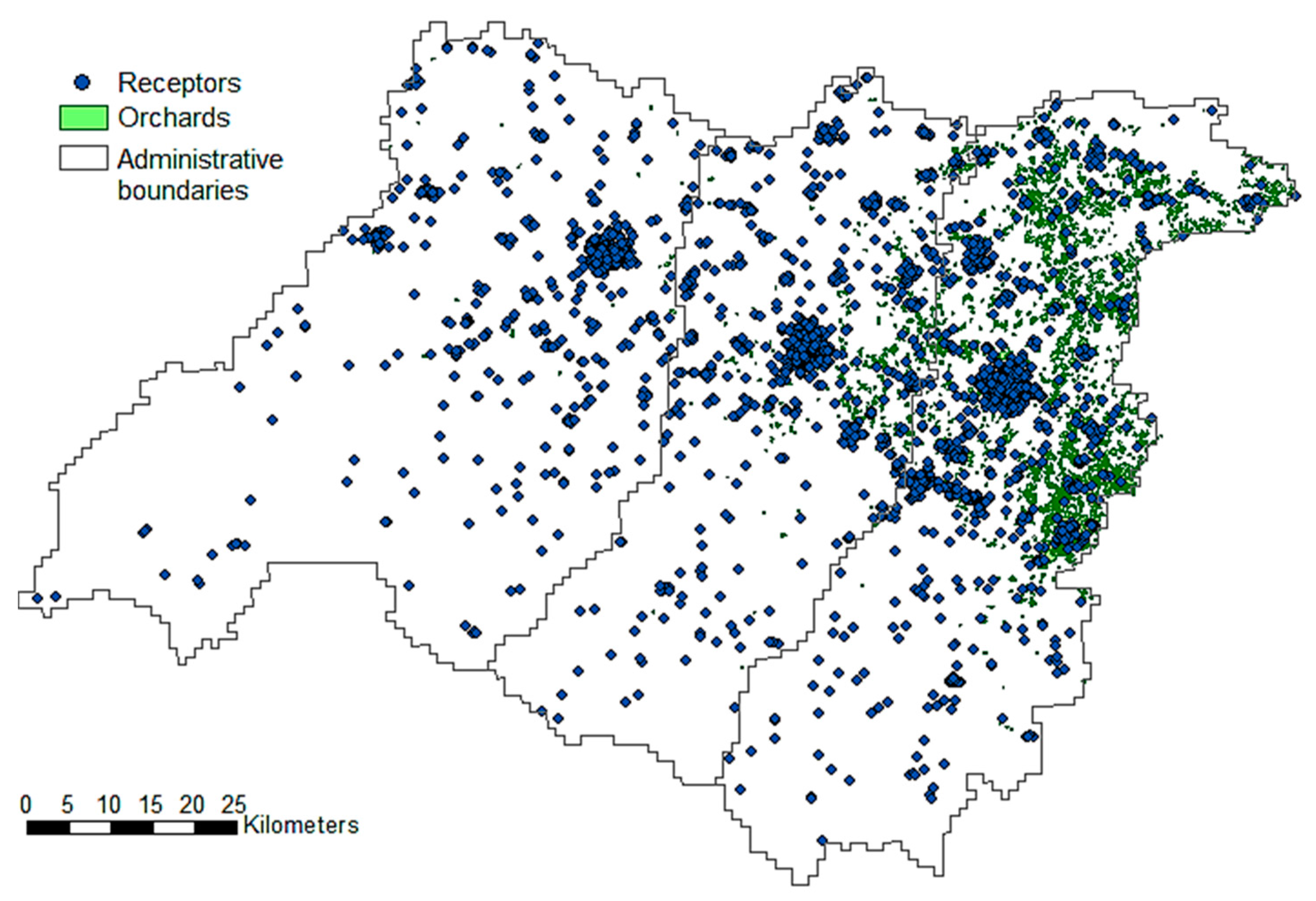
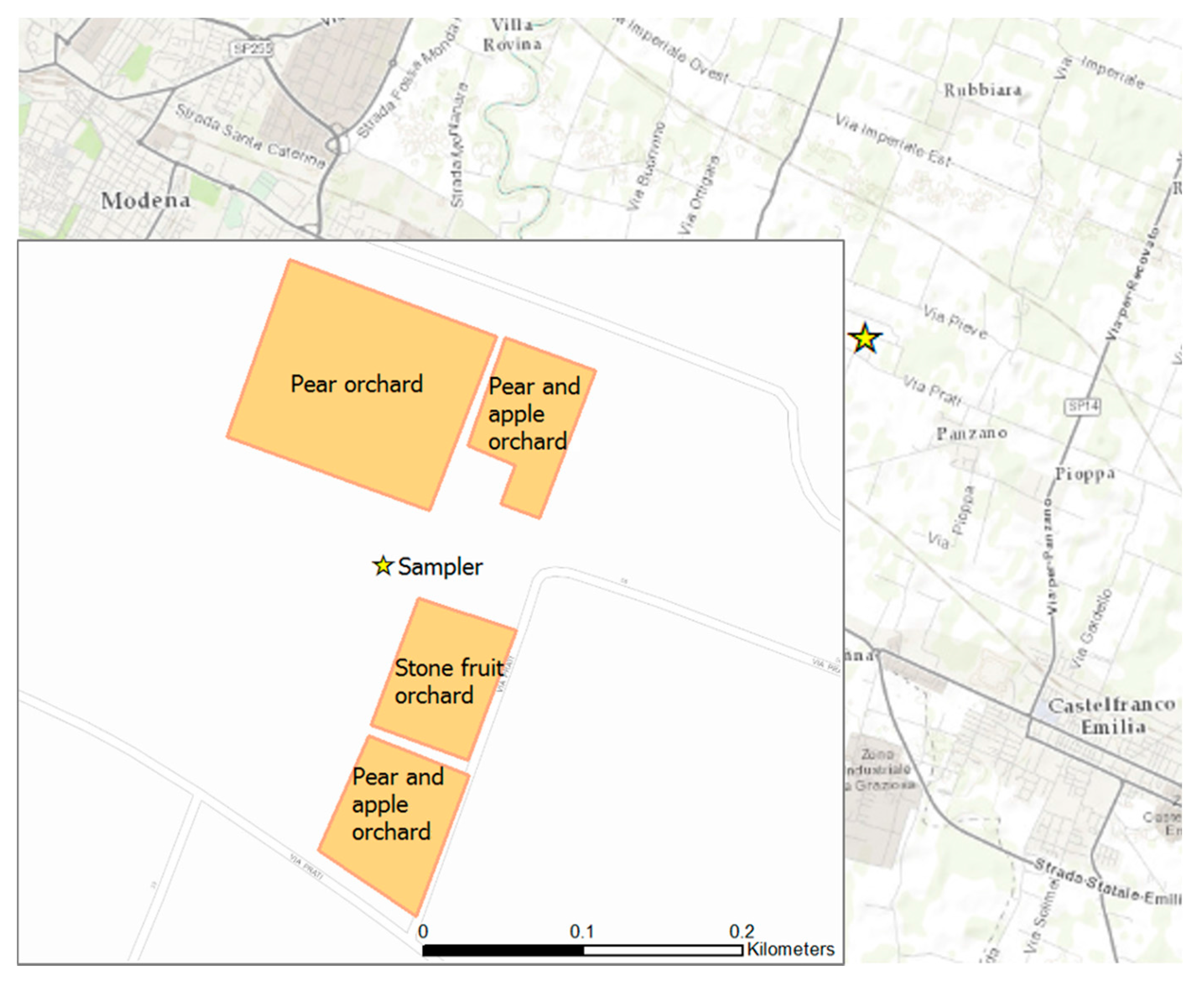
2.1. Geographical Context and Dataset

The study area (Figure 1) is located in the Po Valley (North Italy), and includes the provinces of Modena, Reggio Emilia and Parma covering an area of about 8430 km2. The Po valley experiences a strong anthropic pressure due to wide urban areas, intensive breeding and agriculture (among the most productive agricultural areas within Europe) and wide manufacturing districts, along with topographic and meteorological conditions unfavourable to pollutant dispersion [43,44]. Except to Alps situated north, and the Apennines south of the plain, most of the territory is flat and characterized by a warm temperate subcontinental climate, fully humid, with hot summers (Köppen-Geiger classification Cfa) [45,46]. The climatological pattern of winds for the region is featured by two main wind directions, WNW and ESE, along the longitudinal axis of the Po valley.
The reference population of 2584 people used as target receptors for the assessment of the exposure to pesticides is composed by newly diagnosed ALS cases and up to four age- and sex-matched controls randomly selected from the resident population of the three provinces [47]. Spatially distribution of receptors over the study area is featured by fewer counts in the Southern mountainous part of the area and higher numbers in the surroundings of the main city centres, characterized by a higher population density.
The CORINE Land Cover (CLC) map [48] was used to identify and extract the agricultural fields. The CLC of the studied area was provided by the database of the Geoportal of the Emilia Romagna Region [49]. The land use map of the year 2003 (see 2003 vector land use map, 2011 edition) was chosen for the study because the case/control dataset refers to that period. In this study only the results obtained by considering orchards as risk sources are presented, thus 1519 orchards (polygons) were extracted from the land use database.
A GIS project was setup for the experiment, firstly including the geocoding addresses [50,51] for the localization of the study population and the extraction of orchards from the initial CLC map (Figure 1). Orchards were stored in a shapefile format to be used in the subsequent stages of the work.

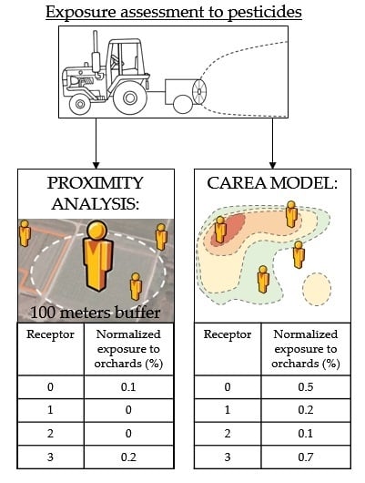
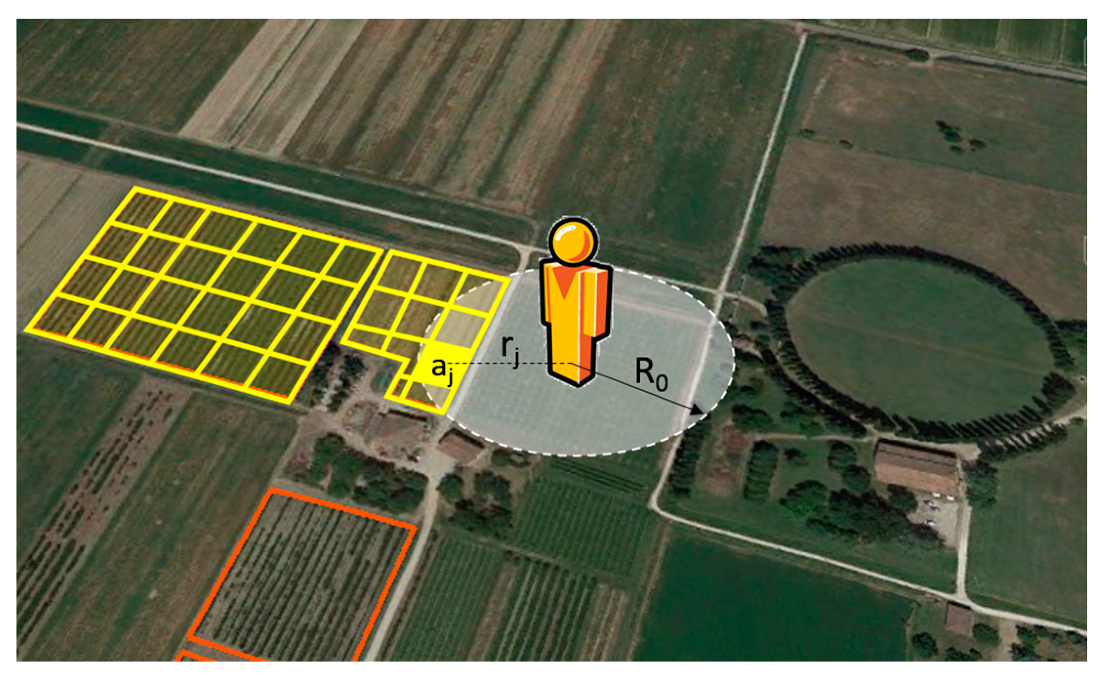
2.2. Proximity Model

GIS spatial analysis techniques are widely used in environmental epidemiology to study the proximity to subjects from the contaminant source, and thus express the proximity as a surrogate for the exposure [52,53,54,55,56].
The proximity model developed in this work is written in Python programming language [28] and consists in the construction of a buffer with a fixed radius (R0) around each receptor (Figure 2).
Polygons of specific land use category are considered as risk sources for the reconstruction of the exposure scenario. Complex polygons with jagged edges, concavities and holes are not supported by the model. Therefore, they were decomposed into simpler geometric entities (i.e., square boxes) with a spatial resolution of 100 m or less. Finally, the exposure of each receptor (see Figure 2) is given by:
E i = A i A n [ 0 , 1 ]
A i = j = 1 N a j ( r j )   j : s . t .   r j R 0
A n = 0 R 0 r d r = π R 0 2
where Ei is the exposure of the receptor i calculated as a normalized areal fraction (between 0 and 1) of the category of agricultural land use considered. Ai is the sum of the risk source areas (aj) found within the buffer of radius R0. An is a normalization factor assumed equal to the area of the buffer of radius R0, while aj is the generic area of a risk source at a distance rj from the receptor.
The model was applied to 2584 receptors and 1519 complex areal sources of orchards using a 100 m buffer as a characteristic distance R0 relying on previous epidemiological studies and literature data [15,20]. Thus, the normalization factor An calculated from a R0 parameter of 100 m became equal to 31,416 m2.

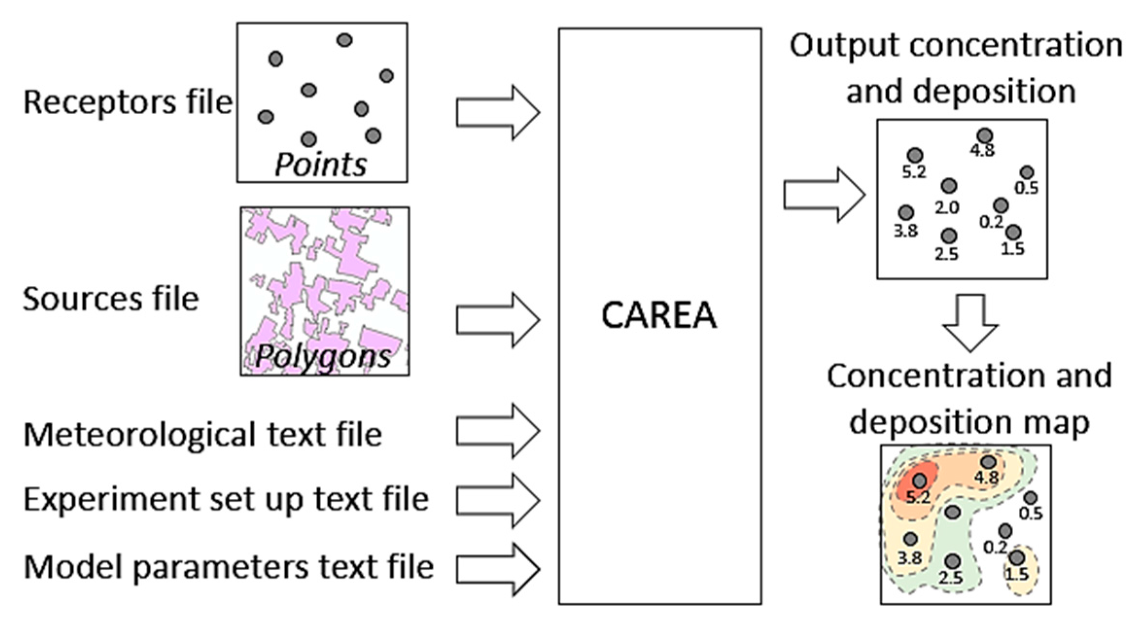
2.3. Atmospheric Dispersion by CAREA

The CAREA model [26] consists in the use of a Gaussian dispersion formulation (mainly based on the simplification of the AERMOD formulation) to simulate mean concentrations and total dry deposition fluxes due to emissions from source areas over flat or hilly domains. CAREA is designed to consider a large number of sources and receptors since existing models are not suitable for large and complex datasets. CAREA is able to simulate domains featured by very complex source polygons with hundreds of vertex and complex geometry. Additionally, definitions of source polygons, source emission rates, receptor locations, output surface concentrations and deposition fluxes can be directly handled in a GIS environment. The CAREA formulation requires several meteorological quantities describing the planetary boundary layer likewise AERMOD. Thus, the meteorological dataset in input to the model is in the AERMET format [27] with hourly data records.
Similar to the proximity model, CAREA was applied to the 2584 receptors and 1519 complex areal sources of the study dataset (CAREA workflow is shown in Figure 3). The model required as input the coordinates of the receptors given by a shapefile containing the receptors listed according to a progressive identifier and with their coordinates as attribute. Orchards polygons were provided through another shapefile where each polygon is characterized by a progressive polygon identifier, a code indicating the land use category (in this case only orchards) and the source emission rate (g m−2 s−1). In this application, an emission rate of 0.001 g s−1 m−2 was used for all the sources, because measured emission values were not available at the moment. Nevertheless, this was not a limiting factor for this study since the relative concentration was used to compare the exposure level among the receptors. Pesticides treatments are not repeated on a daily basis, consequently the simulation of a continuous source may lead to an overestimation of the concentrations at the receptors. However, the re-suspension of a pesticide after its application is a process that needs to be considered [57], thus, suggesting the simulation of a continuous emission source. As a first attempt, neither dry nor wet deposition of dispersed compounds was considered, and no reactivity nor decay of substances was expected. Considering that treatments on orchards (i.e., apple orchards, pear orchards, peach orchards) are done mainly from March to September, the simulation period considered these 7 months, with an hourly time step. Several meteorological data from different sources were used to build the input meteorological file required to CAREA. Meteorological data were selected according to the field campaign carried out in July 2014, i.e., different from the reference period of the case/control dataset, which ranges from the late 90s to the early 2000. However, a multi-annual meteorology can be considered fairly constant over the years. Therefore, the simulation based on the meteorology of year 2014 can be considered representative also for the years 1999–2003. Firstly, the LAMA (Limited Area Meteorological Analysis) dataset [58], created from the simulations of the meteorological model COSMO [59] and the observations of the international meteorological network GTS, was considered. The LAMA dataset is composed by hourly data with an horizontal resolution of 7 km, surface and profile (up to 25 km) parameters, the mixing layer height and other data associated with turbulence. The surface parameters of temperature, humidity, wind intensity and direction were averaged by interfacing the Mantova Belforte LAMA dataset (WGS84 10.5191° E, 45.0611° N) with the data achieved by the ARPAE (Regional Agency for Environmental Protection and Prevention of the Emilia-Romagna region, Italy) stations of Castelfranco Emilia (WGS84 11.029534° E, 44.631303° N) and Modena Urbana (WGS84 10.916985° E, 44.656392° N). Pressure data were supplied by the Osservatorio Geografico of Modena and Reggio Emilia [60,61]. All meteorological data were compliant with the standard of the World Meteorological Organization [62].

2.4. On-Site Measurement Campaign

CAREA results should be validated by ground measurements. Although at the time of the study advanced instrumentation was not available for this operation, a field campaign for the definition and planning of ground measurement of concentration for the validation of CAREA model was performed. In order to have a first inspection on this aspect, pesticide concentrations were measured at a certain distance from orchards fields during a period of treatment.
The measurement campaign took place in Castelfranco Emilia at the experimental farm of the Lazzaro Spallanzani High School (WGS84 11.028876° E, 44.630708° N). This site is located in a rural area 5 km Southeast of Modena. This territory is intensively cultivated with cereal crops (mainly wheat, barley) and some vineyards, apple orchards, pear orchards and peach orchards.
The campaign involved the use of a high volume sampler during the time of application of an insecticide, the emamectin benzoate [63,64,65,66] (Vapour pressure at 21 °C of 4 × 10⁻⁶ Pa, Henry’s law constant at 25 °C and pH 7 of 1.7 × 10⁻⁴ Pa m3/mol, log Pow = 5.0 ± 0,2 at pH 7) on parcels of orchards (see Figure 4). This insecticide belongs to Category 1, the highest toxicity category of the acute toxicity ranking system of the U.S. Environmental Protection Agency [67].
A Total Suspended Particulate (TSP) high volume air sampler (Tisch Environmental Inc., Cleves, OH, USA) with a flow rate between 40 and 60 ft3/min (1.1–1.7 m3/min) equipped with rectangular QM-A quartz fibre filters for aerosols with a thickness of 450 μm (Whatman plc, Maidstone, Kent, UK) was used for the experiment. This instrumentation has been widely described in literature to assess the presence of pesticides residues and other compounds in atmosphere [68,69,70,71,72,73,74,75]. The on-site measurement campaign was carried out in three days, the 30 June, 1 July and 14 July 2014. During the first two days, the atmospheric background concentration of the pesticide was detected. To this aim the sampler was deployed distant from any obstacle in order to work in undisturbed conditions continuously for 24 h. During the second day the air sampling was done simultaneously to the application of the pesticide on orchards parcels. In this case the sampler was placed downwind of the source at variable distances from the atomizer ranging from 100 m to 300 m. The sampling was carried out for the entire duration of treatment in a time period of about 4 h from 11:00 to 15:00 local time of 14 July 2014. Later, the two fibre quartz filters were analysed in order to obtain the mass of emamectin benzoate sampled. An ultrasonic bath with acetonitrile was used to extract the substance from the filters. The extract obtained was suitably diluted and filtered, and thus it was analysed in high performance liquid chromatography coupled with a mass spectrometer detector (LCMS/MS) as described by Vega et al. [76] and others [77,78,79].

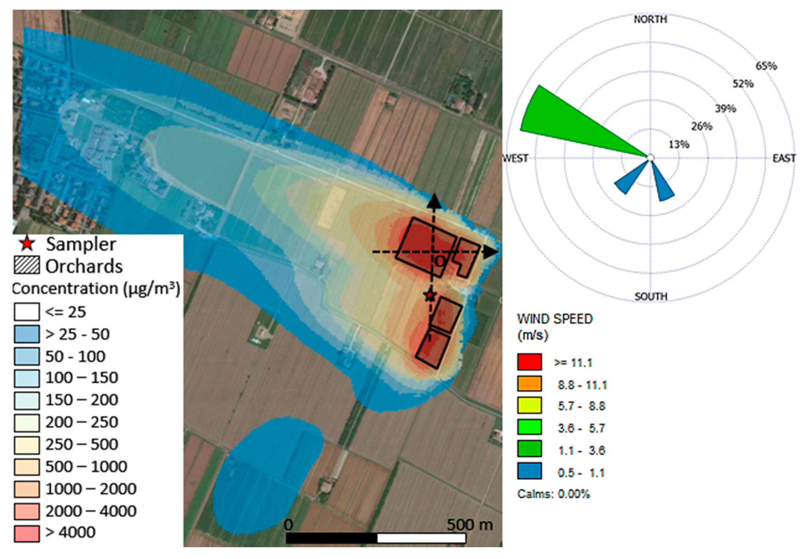
2.5. CAREA Simulation on the Test Site

A CAREA simulation was performed to assess the spatial distribution of the concentration on the test site assuming each orchard as an emission source of pesticide as already discussed in the literature by Wittich et al. [20] and others [80,81].
The simulation was setup in order to consider both the spray drift at the time of application and the re-suspension of the pesticide after its application. The latter process was modelled assuming fields as emission sources even after the application of the pesticides. To this aim, the simulation was carried out in four separate runs, because four fields (one pear orchard, two pear and apple orchards and one stone fruit orchard) were involved in the application of the pesticide during the experiment. The pesticide was applied clockwise starting from the upper left pear orchard (source 1) up to the southernmost pear orchard (source 4). Therefore, the first run involved only the contribution of the source 1, while the second run involved the contribution of the source 1 and 2. Consistently, the last run involved the contribution of all the sources. The simulation was setup considering a computational domain of 2.5 × 2.5 km2 focused on the farm. Similarly to the simulation showed in sections above, a source emission rate of 0.001 g s−1 m−2 was used as default value for all the sources. For simplicity, neither dry nor wet deposition of the pesticide was considered, as well as neither reactivity nor decay of emamectin benzoate was expected. Additional simulation parameters involved the use of a simulation period of four hours from 11:00 to 15:00 of 14 July 2014.
Finally, the four outputs of the simulations were summed to a total concentration map. This latter output was spatially interpolated by the application of the Kriging method [82] to obtain the final concentration map over the simulation domain.

3. Results and Discussion

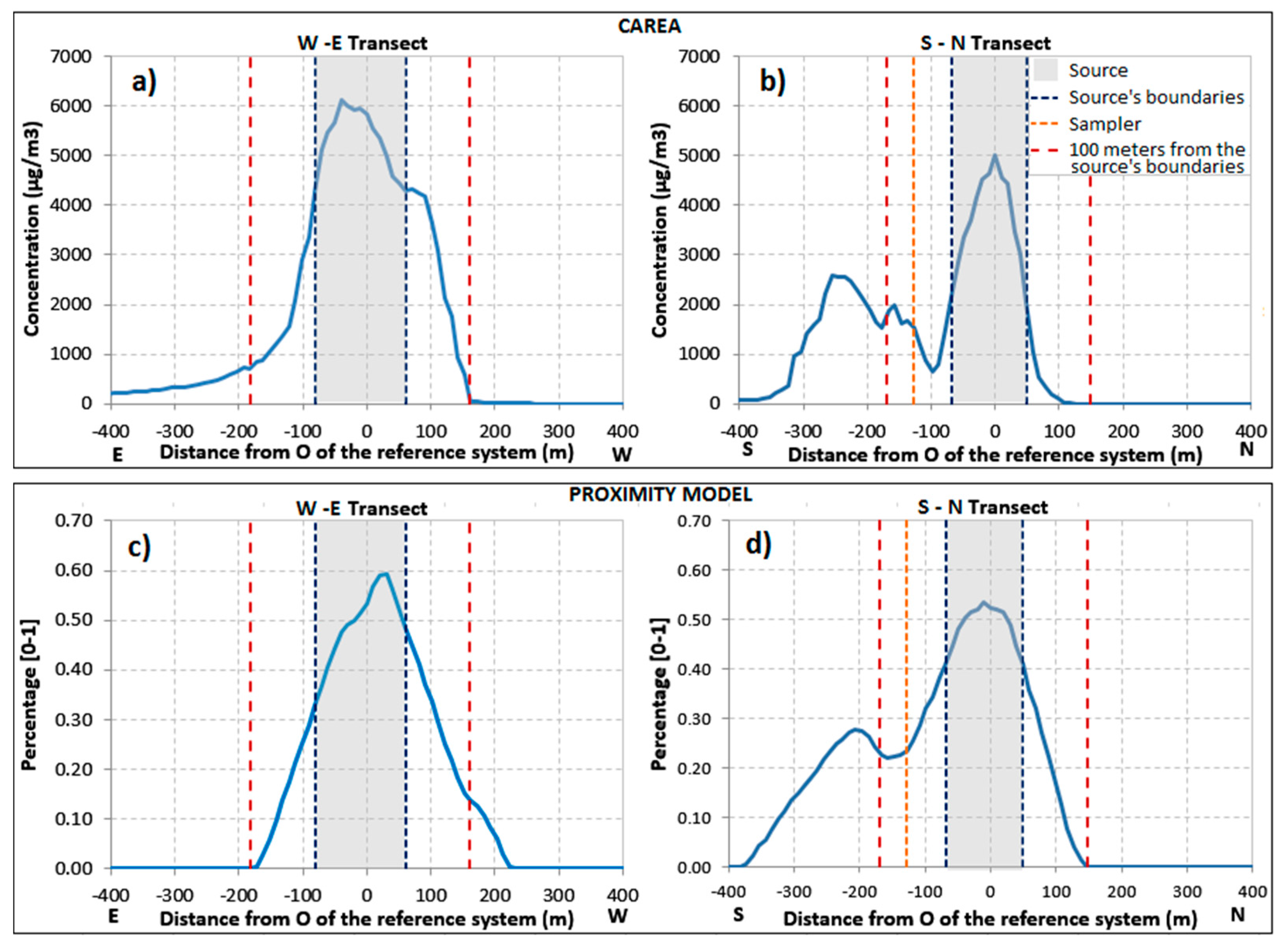
3.1. Comparison between the Proximity Model and the CAREA Model

The exposure of the receptors provided by the proximity model is expressed by a normalized areal fraction of the orchards land use found within the buffer of 100 m. Normalized exposure ranges from 0, no areal percentage of orchards within the searching distance, to 1, full presence of orchards within the buffer. Here, receptors with exposure equal to 0 were defined as not-exposed. The discussion of the results obtained by the proximity model from the epidemiological point of view for this case study was presented by Vinceti et al. [47]. The CAREA output provided, for each receptor, a relative concentration value (C) assumed proportional to the receptor exposure to orchards and the concentration ratio (Ĉ), which is a normalization of the concentration of the receptor according to a reference case. More specifically, Ĉ was calculated by the ratio between the relative concentration value (C) of a receptor and the reference concentration C0 estimated as follows: firstly, a circumference centred at the receptor with a radius of 100 m was considered, then the model was run by using the same meteorological conditions. Thus, C0 is the maximum concentration of hypothetical receptors which are located at a distance of 100 m from the polygon considered. Basically, if Ĉ is equal to 2, it means that the considered receptor has a double concentration respect to the reference case. Receptors with Ĉ less than 1 were defined as not-exposed.
Here, in order to evaluate the differences in terms of exposure of receptors, exposure data calculated by the two models were split and encoded into five risk classes: the code “−999” was assigned to not-exposed receptors, while the classes “0, 1, 2, 3” were used to encode normalized exposures between the ranges (0, 0.25), (0.25, 0.5), (0.5, 0.75), (0.75, 1.00), respectively.
Observing Table 1, it can be stated that CAREA output resulted in a greater distribution of the receptors among the exposure classes than the proximity model. In particular, the not-exposed receptors decrease from the 96% of the proximity model to the 46% of the CAREA model. This is a consequence of their different formulation, with the proximity model considering an exposure distance of only 100 m and with CAREA simulating the Gaussian atmospheric dispersion of the pesticide up to few kilometres. Moreover, it can be stated that the differences between the two models become smaller at high exposures. Especially, when exposure classes “2” and “3” are considered, exposures provided by the two models are very similar. This latter aspect leads to a greater protection for the receptors, because at high exposure levels the output provided is less dependent on the chosen approach.

3.2. CAREA Simulation on the Test Site

Figure 5 shows how the dispersion of the pesticide is strongly affected by the meteorological conditions, with a well-developed plume along the main wind direction (see associated wind rose). Moreover, two transects (see Figure 5) were extracted along the S-N and W-E directions centred on the sampler. Figure 6 shows CAREA concentrations and the results of the application of the proximity model of hypothetical receptors obtained from the discretization of the transects with a step of 10 m.
The concentration map over the simulation domain retrieved by CAREA is reported below.
The transport of the pesticide due to the mean wind direction is also verifiable by observing the trend along the W-E transect calculated by CAREA (Figure 6a) compared to the one achieved by the proximity model (Figure 6c). Figure 6a shows significant pesticide concentrations (1/5 of the maximum value) up to 100 m from the source’s boundaries (see dotted red line at about-200 m from the origin of the reference system), while the same point has near to zero values in the proximity model (Figure 6c). Similarly, no concentrations were computed by CAREA for hypothetical receptors placed downwind at about 200 m from the origin of the reference system (see right dotted red line), while significant values were computed by the proximity model. The comparison of the trends along the S-N transect of the two models shows minor differences because this direction is less affected by the mean wind; e.g., these trends showed a bimodal distribution with two peaks right and left from the sampler (dotted orange line) probably due to the two sources (fields) that are present north and south from the sampler itself.
Briefly, exposure scenarios derived from the models showed some peculiarities. The use of a proximity model instead of the CAREA model at the scale of this experiment led to a slight underestimation/overestimation of the exposure, but, if a wider area it is considered, it is reasonable to expect a larger discrepancy. Near to zero concentrations found up to distance of 300 m from the treated field (see left branch of Figure 6a) may become very significant if more sources and receptors are considered. Hence, the effects of meteorology led to a site-specific exposure distribution that substantially differs from the symmetric one on which proximity models are based.

3.3. On-Site Measurement Campaign

The field campaign was performed for the definition and planning of ground measurement of concentration for the validation of CAREA model. The two fibre quartz filters were analysed in order to obtain the mass of emamectin benzoate sampled during the background concentration measurement and during the application of the pesticide. The laboratory reported a Detection Limit (LD) for emamectin benzoate of 0.25 ppb and a Quantification Limit (LQ) of 0.50 ppb. The analysis of the blank filter reported no mass of emamectin benzoate. Contrariwise, a mass of 0.97 ± 0.31 µg was found in the filter sampled during orchards treatment with the pesticide. By estimating the flow rate of the high-volume sampler in about 1.4 m3/min, the observed atmospheric concentration of emamectin benzoate was of 0.02 ng/m3. Literature experiments reported ambient air in concentrations ranging from few pg/m3 to several ng/m3 [72,73,83,84,85,86,87,88], but each study showed its own peculiarities. In particular, the sampled pesticides often have different chemical and physical characteristics, the use of several types of sampling equipment and application techniques, the different weather conditions, etc. To date, the retrieved quantity is consistent with the data found in the literature, notwithstanding the differences between the several experiments. As shown in Figure 6b, the trend along the S-N transect is characterized by two peaks right and left from the sampler, thus the sampled concentration may be slightly underestimated.
Moreover, from a qualitatively point of view, the results of the campaign showed pesticide concentrations that differ substantially from the background values. Study outlooks include a further development of the validation of the CAREA model by the use of suitable instrumentation to achieve reliable ground measurements.

4. Conclusions

The use of the CAREA atmospheric dispersion model led to a considerable enhancement in the percentage of exposed receptors, from the 4% of the proximity model to the 54% of the CAREA model. This is a consequence due to the formulation of the models, with a short computing distance of 100 m for the proximity model and the use of an atmospheric dispersion model able to simulate the dispersion of pollutant up to few kilometres for the CAREA model. Moreover, it can be observed that the differences between the two models become smaller for high exposures. This latter aspect leads to a greater protection for the receptors, because at high exposure levels the output provided by the two models is less dependent to the chosen approach.
A CAREA simulation was performed to assess the spatial distribution of the pesticide concentration over a test site chosen to achieve a preliminary ground measurement of concentration for the validation of CAREA model. The concentration map over the simulation domain shows that pesticide dispersion is strongly affected by meteorological conditions with a well-developed plume along the main wind direction. Then, CAREA concentrations and normalized exposures by the proximity model of hypothetical receptors obtained from the discretization of the W-E and S-N transects were compared. The use of a proximity model instead of the CAREA model at the scale of this experiment led to a slight underestimation/overestimation of the exposure, but, if a wider area is considered, it is reasonable to expect a larger discrepancy. Near to zero concentrations found up to distance of 300 m from the treated field (see left branch of the W-E CAREA transect) may become very significant if more sources and receptors are considered. Hence, the effects of meteorology led to a site-specific exposure distribution that substantially differs from the symmetric one on which proximity models are based. This aspect should be taken into account when the environmental impact of a substance is assessed both in terms of added value of one study (better approximation of the real exposure of receptors) and to protect people’s health. The CAREA model should be used also in the toxicological approach because it provides an estimation of the site-measured concentration of a substance.
The discussion of the results obtained by the proximity model from the epidemiological point of view for this case study was presented in literature by Vinceti et al. [47]. Future outlooks include the use of the exposure scenario evaluated by CAREA in the aforementioned study. Moreover, both models will be used in other activities, such as the population exposure assessment from cyanobacteria from inland waters.
Finally, the results of the on-site measurement campaign showed how, during treatments, pesticide concentrations distant from the fields are significantly higher than background values. To date, the retrieved quantity seems to be consistent with the data found in literature, but with all the uncertainness related to the differences of the various experiments. Future outlooks include a further development of the validation of the CAREA model by the use of suitable instrumentation to achieve reliable ground measurements.

Acknowledgments

This study has been supported also by FCRM (Fondazione Cassa di Risparmio di Modena) in the frame of the project “Esposizione ai pesticidi usati in agricoltura: metodologia avanzata di valutazione e rischio sanitario.”

Author Contributions

S.C. and S.T. were the coordinators of the whole activity; they developed the CAREA model, did the GIS proximity analysis study, designed the experiment, and wrote the paper. G.G. contributed to the analysis of the atmospheric dispersion model results, and to prepare the paper. A.B. and R.N. were responsible of the field campaign: R.N. organized the campaign and A.B. setup the experiment and analysed the samples. T.F., C.M. and M.V. were responsible of the epidemiological application of the results: specifically, M.V. coordinated de epidemiological group and analysed and defined the exposure levels (classes), T.F. and C.M. were involved in the building of the case/control dataset.

Conflicts of Interest

The authors declare no conflict of interest.

References

  1. Townson, H. Public health impact of pesticides used in agriculture. Trans. R. Soc. Trop. Med. Hyg. 1992, 86, 350. [Google Scholar] [CrossRef]
  2. Gil, Y.; Sinfort, C. Emission of pesticides to the air during sprayer application: A bibliographic review. Atmos. Environ. 2005, 39, 5183–5193. [Google Scholar] [CrossRef]
  3. Margni, M.; Rossier, D.; Crettaz, P.; Jolliet, O. Life cycle impact assessment of pesticides on human health and ecosystems. Agric. Ecosyst. Environ. 2002, 93, 379–392. [Google Scholar] [CrossRef]
  4. Damalas, C.A.; Eleftherohorinos, I.G. Pesticide exposure, safety issues, and risk assessment indicators. Int. J. Environ. Res. Public Health 2011, 8, 1402–1419. [Google Scholar] [CrossRef] [PubMed]
  5. Van Der Werf, H.M.G. Assessing the impact of pesticides on the environment. Agric. Ecosyst. Environ. 1996, 60, 81–96. [Google Scholar] [CrossRef]
  6. Levitan, L.; Merwin, I.; Kovach, J. Assessing the relative environmental impacts of agricultural pesticides: The quest for a holistic method. Agric. Ecosyst. Environ. 1995, 55, 153–168. [Google Scholar] [CrossRef]
  7. Zauli Sajani, S.; Forti, S.; Lauriola, P. Benzene exposure in Modena: Historical trend and health risk assessment. Epidemiol. Prev. 2005, 29, 13–18. [Google Scholar] [PubMed]
  8. Mattison, D.R.; Sandler, J.D. Summary of the workshop on issues in risk assessment: Quantitative methods for developmental toxicology. Risk Anal. 1994, 14, 595–604. [Google Scholar] [CrossRef] [PubMed]
  9. Agenzia per la Protezione, dell’Ambiente e per i Servizi Tecnici (Apat). Criteri Metodologici per L’applicazione Dell’analisi Assoluta di Rischio ai siti Contaminati. Rome, 2008. Available online: https://www.google.com.sg/url?sa=t&rct=j&q=&esrc=s&source=web&cd=2&ved=0ahUKEwj5zfyuwu_YAhXDNpQKHZTqDIsQFgguMAE&url=http%3A%2F%2Fwww.isprambiente.gov.it%2Ffiles%2Ftemi%2Fsiti-contaminati-02marzo08.pdf&usg=AOvVaw3U7EIHq1t_yKh_B4u5vIVt (accessed on 23 January 2018).
  10. Samet, J.M.; Schnatter, R.; Gibb, H. Invited commentary: Epidemiology and risk assessment. Am. J. Epidemiol. 1998, 148, 929–936. [Google Scholar] [CrossRef] [PubMed]
  11. Goodchild, M.F. Geographic information systems and science: Today and tomorrow. Procedia Earth Planet. Sci. 2009, 1, 1037–1043. [Google Scholar] [CrossRef]
  12. Auchincloss, A.H.; Gebreab, S.Y.; Mair, C.; Diez Roux, A.V. A Review of Spatial Methods in Epidemiology, 2000–2010. Annu. Rev. Public Health 2012, 33, 107–122. [Google Scholar] [CrossRef] [PubMed]
  13. Jacquez, G.M. Spatial analysis in epidemiology: Nascent science or a failure of GIS? J. Geogr. Syst. 2000, 2, 91–97. [Google Scholar] [CrossRef]
  14. Nuckols, J.R.; Ward, M.H.; Jarup, L. Using geographic information systems for exposure assessment in environmental epidemiology studies. Environ. Health Perspect. 2004, 112, 1007–1015. [Google Scholar] [CrossRef] [PubMed]
  15. Malagoli, C.; Costanzini, S.; Heck, J.E.; Malavolti, M.; De Girolamo, G.; Oleari, P.; Palazzi, G.; Teggi, S.; Vinceti, M. Passive exposure to agricultural pesticides and risk of childhood leukemia in an Italian community. Int. J. Hyg. Environ. Health 2016, 219, 742–748. [Google Scholar] [CrossRef] [PubMed]
  16. Ranzi, A.; Cordioli, M. Metodi e approcci per l’analisi quantitativa. Ecoscenza 2014, 4, 98–99. [Google Scholar]
  17. Johnson, B.; Barry, T.; Wofford, P. Workbook for Gaussian Modeling Analysis of Air Concentration Measurements Workbook for Gaussian Modeling Analysis of Air Concentration Measurements; Environmental Protection Agency, Department of Pesticide Regulation Environmental, Monitoring Branch: Sacramento, CA, USA, 2010.
  18. Smith, R.J. A Gaussian model for estimating odour emissions from area sources. Math. Comput. Model. 1995, 21, 23–29. [Google Scholar] [CrossRef]
  19. Tsai, M.Y.; Elgethun, K.; Ramaprasad, J.; Yost, M.G.; Felsot, A.S.; Hebert, V.R.; Fenske, R.A. The Washington aerial spray drift study: Modeling pesticide spray drift deposition from an aerial application. Atmos. Environ. 2005, 39, 6194–6203. [Google Scholar] [CrossRef]
  20. Wittich, K.P.; Siebers, J. Aerial short-range dispersion of volatilized pesticides from an area source. Int. J. Biometeorol. 2002, 46, 126–135. [Google Scholar] [CrossRef] [PubMed]
  21. Ghermandi, G.; Teggi, S.; Fabbi, S.; Bigi, A.; Cecchi, R. Model comparison in simulating the atmospheric dispersion of a pollutant plume in low wind conditions. Int. J. Environ. Pollut. 2012, 48, 69. [Google Scholar] [CrossRef]
  22. Karamchandani, P.; Vijayaraghavan, K.; Yarwood, G. Sub-grid scale plume modeling. Atmosphere 2011, 2, 389–406. [Google Scholar] [CrossRef]
  23. Teske, M.E.; Bird, S.L.; Esterly, D.M.; Curbishley, T.B.; Ray, S.L.; Perry, S.G. AgDrift®: A model for estimating near-field spray drift from aerial applications. Environ. Toxicol. Chem. 2002, 21, 659–671. [Google Scholar] [CrossRef] [PubMed]
  24. Bilanin, A.J.; Teske, M.E.; Barry, J.W.; Ekblad, R.B. AGDISP: The Aircraft Spray Dispersion Model, Code Development and Experimental Validation. Trans. ASABE 1989, 32, 327–334. [Google Scholar] [CrossRef]
  25. Reiss, R.; Griffin, J. A probabilistic model for acute bystander exposure and risk assessment for soil fumigants. Atmos. Environ. 2006, 40, 3548–3560. [Google Scholar] [CrossRef]
  26. Teggi, S.; Costanzini, S.; Ghermandi, G.; Malagoli, C.; Vinceti, M. A GIS-based atmospheric dispersion model for pollutants emitted by complex source areas. Sci. Total Environ. 2018, 610–611, 175–190. [Google Scholar] [CrossRef] [PubMed]
  27. Cimorelli, A.J.; Perry, S.G.; Venkatram, A.; Weil, J.C.; Paine, R.J.; Wilson, R.B.; Lee, R.F.; Peters, W.D.; Brode, R.W.; Paumier, J.O. AERMOD: Description of Model Formulation; Report; Scholar’s Choice: London, ON, Canada, 2004; Volume 44, pp. 1–91. [Google Scholar]
  28. Python Software Foundation. Python Language Reference, Version 2.7; Python Software Foundation: Wilmington, DE, USA, 2013. [Google Scholar]
  29. Batiha, M.A.; Al-Makhadmeh, L.A.; Batiha, M.M.; Ramadan, A.; Kadhum, A.A.H. Generalization of the mafram methodology for semi-volatile organic agro-chemicals. Water. Air. Soil Pollut. 2014, 225. [Google Scholar] [CrossRef]
  30. Batiha, M.A.; Kadhum, A.A.H.; Batiha, M.M.; Takriff, M.S.; Mohamad, A.B. MAFRAM-A new fate and risk assessment methodology for non-volatile organic chemicals. J. Hazard. Mater. 2010, 181, 1080–1087. [Google Scholar] [CrossRef] [PubMed]
  31. Nimmatoori, P.; Kumar, A. Development and evaluation of a ground-level area source analytical dispersion model to predict particulate matter concentration for different particle sizes. J. Aerosol Sci. 2013, 66, 139–149. [Google Scholar] [CrossRef]
  32. Nimmatoori, P.; Kumar, A. Evaluation of area source models to predict near ground level concentrations due to emissions released during agricultural applications. J. Hazard. Mater. 2013, 246–247, 44–51. [Google Scholar] [CrossRef] [PubMed]
  33. Pivato, A.; Barausse, A.; Zecchinato, F.; Palmeri, L.; Raga, R.; Lavagnolo, M.C.; Cossu, R. An integrated model-based approach to the risk assessment of pesticide drift from vineyards. Atmos. Environ. 2015, 111, 136–150. [Google Scholar] [CrossRef]
  34. Van den Berg, F.; Jacobs, C.M.J.; Butler Ellis, M.C.; Spanoghe, P.; Doan Ngoc, K.; Fragkoulis, G. Modelling exposure of workers, residents and bystanders to vapour of plant protection products after application to crops. Sci. Total Environ. 2016, 573, 1010–1020. [Google Scholar] [CrossRef] [PubMed]
  35. Martinez, A.; Spak, S.N.; Petrich, N.T.; Hu, D.; Carmichael, G.R.; Hornbuckle, K.C. Atmospheric dispersion of PCB from a contaminated Lake Michigan harbor. Atmos. Environ. 2015, 122, 791–798. [Google Scholar] [CrossRef] [PubMed]
  36. Bauer, T.J. Comparison of chlorine and ammonia concentration field trial data with calculated results from a Gaussian atmospheric transport and dispersion model. J. Hazard. Mater. 2013, 254–255, 325–335. [Google Scholar] [CrossRef] [PubMed]
  37. Llanos, W.; Kocman, D.; Higueras, P.; Horvat, M. Mercury emission and dispersion models from soils contaminated by cinnabar mining and metallurgy. J. Environ. Monit. 2011, 13, 3460–3468. [Google Scholar] [CrossRef] [PubMed]
  38. Tartakovsky, D.; Stern, E.; Broday, D.M. Dispersion of TSP and PM10 emissions from quarries in complex terrain. Sci. Total Environ. 2016, 542, 946–954. [Google Scholar] [CrossRef] [PubMed]
  39. Tartakovsky, D.; Stern, E.; Broday, D.M. Indirect estimation of emission factors for phosphate surface mining using air dispersion modeling. Sci. Total Environ. 2016, 556, 179–188. [Google Scholar] [CrossRef] [PubMed]
  40. Brianza, M. Distribuzione dei Fitofarmaci: Stato Dell’ Arte e Impiego di Attrezzature Intelligenti per il Contenimento dei Costi e il Miglioramento Della Sostenibilità Delle Produzioni Vitivinicole Milanesi e Lombarde; Coldiretti: Monza Brianza, Italy, 2015; ISBN 978-88-9-407222-8. [Google Scholar]
  41. Hall, F.R.; Chapple, A.C.; Downer, R.A.; Kirchner, L.M.; Thacker, J.R.M. Pesticide application as affected by spray modifiers. J. Pestic. Sci. 1993, 38, 123–133. [Google Scholar] [CrossRef]
  42. Hilz, E.; Vermeer, A.W.P. Spray drift review: The extent to which a formulation can contribute to spray drift reduction. Crop Prot. 2013, 44, 75–83. [Google Scholar] [CrossRef]
  43. Bigi, A.; Ghermandi, G.; Harrison, R.M. Analysis of the air pollution climate at a background site in the Po valley. J. Environ. Monit. 2012, 14, 552–563. [Google Scholar] [CrossRef] [PubMed] [Green Version]
  44. Bocchiola, D.; Nana, E.; Soncini, A. Impact of climate change scenarios on crop yield and water footprint of maize in the Po valley of Italy. Agric. Water Manag. 2013, 116, 50–61. [Google Scholar] [CrossRef]
  45. Peel, M.C.; Finlayson, B.L.; McMahon, T.A. Updated world map of the Köppen-Geiger climate classification. Hydrol. Earth Syst. Sci. Discuss. 2007, 4, 439–473. [Google Scholar] [CrossRef]
  46. Rubel, F.; Kottek, M. Observed and projected climate shifts 1901–2100 depicted by world maps of the Köppen-Geiger climate classification. Meteorol. Z. 2010, 19, 135–141. [Google Scholar] [CrossRef]
  47. Vinceti, M.; Filippini, T.; Violi, F.; Rothman, K.J.; Costanzini, S.; Malagoli, C.; Wise, L.A.; Odone, A.; Signorelli, C.; Iacuzio, L.; et al. Pesticide exposure assessed through agricultural crop proximity and risk of amyotrophic lateral sclerosis. Environ. Health 2017, 16, 91. [Google Scholar] [CrossRef] [PubMed]
  48. Bossard, M.; Feranec, J.; Otahel, J. CORINE Land Cover Technical Guide—Addendum 2000; Technical Report; No. 105; European Eviroment Agency: Copenhagen, Denmark, 2000. [Google Scholar]
  49. Geoportale Della Regione Emilia Romagna. Available online: https://geoportale.regione.emilia-romagna.it/it (accessed on 12 October 2017).
  50. Ward, M.H.; Nuckols, J.R.; Giglierano, J.; Bonner, M.R.; Wolter, C.; Airola, M.; Mix, W.; Colt, J.S.; Hartge, P. Positional Accuracy of Two Methods of Geocoding. Epidemiology 2005, 16, 542–547. [Google Scholar] [CrossRef] [PubMed]
  51. Bonner, M.R.; Han, D.; Nie, J.; Rogerson, P.; Vena, J.E.; Freudenheim, J.L. Positional accuracy of geocoded addresses in epidemiologic research. Epidemiology 2003, 14, 408–412. [Google Scholar] [CrossRef] [PubMed]
  52. Bell, E.M.; Hertz-Picciotto, I.; Beaumont, J.J. A case-control study of pesticides and fetal death due to congenital anomalies. Epidemiology 2001, 12, 148–156. [Google Scholar] [CrossRef] [PubMed]
  53. Comba, P.; Ascoli, V.; Belli, S.; Benedetti, M.; Gatti, L.; Ricci, P.; Tieghi, A. Risk of soft tissue sarcomas and residence in the neighbourhood of an incinerator of industrial wastes. Occup. Environ. Med. 2003, 60, 680–683. [Google Scholar] [CrossRef] [PubMed]
  54. Xiang, H.; Nuckols, J.R.; Stallones, L. A geographic information assessment of birth weight and crop production patterns around mother’s residence. Environ. Res. 2000, 82, 160–167. [Google Scholar] [CrossRef] [PubMed]
  55. Gunier, R.B.; Ward, M.H.; Airola, M.; Bell, E.M.; Colt, J.; Nishioka, M.; Buffler, P.A.; Reynolds, P.; Rull, R.P.; Hertz, A.; et al. Determinants of agricultural pesticide concentrations in carpet dust. Environ. Health Perspect. 2011, 119, 970–976. [Google Scholar] [CrossRef] [PubMed]
  56. Nuckols, J.R.; Gunier, R.B.; Riggs, P.; Miller, R.; Reynolds, P.; Ward, M.H. Linkage of the California Pesticide Use Reporting Database with spatial land use data for exposure assessment. Environ. Health Perspect. 2007, 115, 684–689. [Google Scholar] [CrossRef] [PubMed]
  57. Thatcher, T.L.; Layton, D.W. Deposition, resuspension, and penetration of particles within a residence. Atmos. Environ. 1995, 29, 1487–1497. [Google Scholar] [CrossRef]
  58. ARPA Regional Agency for Environmental Protection and Prevention in the Emilia-Romagna Region, I. LAMA. Available online: https://www.arpae.it/cms3/documenti/_cerca_doc/meteo/ambiente/descrizione_lama.pdf (accessed on 2 January 2018).
  59. Rockel, B.; Will, A.; Hense, A. The Regional Climate Model COSMO-CLM. Meteorol. Z. 2008, 17, 347–348. [Google Scholar] [CrossRef]
  60. Lombroso, L.; Quattrocchi, S. L’osservatorio di MODENA: 180 Anni di Misure Meteoclimatiche; Societa Meteorologica Subalpina: Moncalieri, Italy, 2008; ISBN 978-88-9-030232-9. [Google Scholar]
  61. Lombroso, L.; Teggi, S. Annuario delle osservazioni meteoclimatiche dell’anno 2014 all’Osservatorio Geofisico di Modena. Società dei Naturalisti e Matematici di Modena 2015, 146, 25–36. [Google Scholar]
  62. Bekiashev, K.A.; Serebriakov, V.V. World Meteorological Organization (WMO). In International Marine Organizations; Springer: Berlin/Heidelberg, Germany, 1981; pp. 540–552. [Google Scholar]
  63. Zhu, J.; He, Y.; Gao, M.; Zhou, W.; Hu, J.; Shen, J.; Zhu, Y.C. Photodegradation of emamectin benzoate and its influence on efficacy against the rice stem borer, Chilo suppressalis. Crop Prot. 2011, 30, 1356–1362. [Google Scholar] [CrossRef]
  64. Ishaaya, I.; Kontsedalov, S.; Horowitz, A.R. Emamectin, a novel insecticide for controlling field crop pests. Pest Manag. Sci. 2002, 58, 1091–1095. [Google Scholar] [CrossRef] [PubMed]
  65. Jansson, R.K.; Peterson, R.F.; Halliday, W.R.; Mookerjee, P.K.; Dybas, R.A. Efficacy of solid formulations of emamectin benzoate at controlling lepidopterous pests. Fla. Entomol. 1996, 79, 434–449. [Google Scholar] [CrossRef]
  66. Jansson, R.K.; Brown, R.; Cartwright, B.; Cox, D.; Dunbar, D.M.; Dybas, R.A.; Eckel, C.; Lasota, J.A.; Mookerjee, P.K.; Norton, J.A.; et al. Emamectin benzoate: A novel avermectin derivative for control of lepidopterous pests. In Proceedings of the 3rd International Workshop Management of Diamondback Moth Other Crucifer Pests, Kuala Lumpur, Malaysia, 29 October–1 November 1997; pp. 172–177. [Google Scholar]
  67. EPA Chemical Hazard Classification and Labeling: Comparison of Requirements and the GHS. Available online: https://www.epa.gov/sites/production/files/2015-09/documents/ghscriteria-summary.pdf (accessed on 9 January 2018).
  68. König, J.; Funcke, W.; Balfanz, E.; Grosch, B.; Pott, F. Testing a high volume air sampler for quantitative collection of polycyclic aromatic hydrocarbons. Atmos. Environ. 1980, 14, 609–613. [Google Scholar] [CrossRef]
  69. Bidleman, T.F.; Olney, C.E. High-volume collection of atmospheric polychlorinated biphenyls. Bull. Environ. Contam. Toxicol. 1974, 11, 442–450. [Google Scholar] [CrossRef] [PubMed]
  70. Hayward, S.J.; Gouin, T.; Wania, F. Comparison of Four Active and Passive Sampling Techniques for Pesticides in Air. Environ. Sci. Technol. 2010, 44, 3410–3416. [Google Scholar] [CrossRef] [PubMed]
  71. Scheyer, A.; Morville, S.; Mirabel, P.; Millet, M. Variability of atmospheric pesticide concentrations between urban and rural areas during intensive pesticide application. Atmos. Environ. 2007, 41, 3604–3618. [Google Scholar] [CrossRef]
  72. Coscollà, C.; Hart, E.; Pastor, A.; Yusà, V. LC-MS characterization of contemporary pesticides in PM10 of Valencia Region, Spain. Atmos. Environ. 2013, 77, 394–403. [Google Scholar] [CrossRef]
  73. Aulagnier, F.; Poissant, L.; Brunet, D.; Beauvais, C.; Pilote, M.; Deblois, C.; Dassylva, N. Pesticides measured in air and precipitation in the Yamaska Basin (Québec): Occurrence and concentrations in 2004. Sci. Total Environ. 2008, 394, 338–348. [Google Scholar] [CrossRef] [PubMed]
  74. Hart, K.M.; Pankow, J.F. High-Volume Air Sampler for Particle and Gas Sampling. 2. Use of Backup Filters To Correct for the Adsorption of Gas-Phase Polycyclic Aromatic Hydrocarbons to the Front Filter. Environ. Sci. Technol. 1994, 28, 655–661. [Google Scholar] [CrossRef] [PubMed]
  75. Cessna, A.J.; Waite, D.T.; Bailey, J.; Kerr, L.A.; Quiring, D.V. Desorption of herbicides from atmospheric particulates during high-volume air sampling. Atmosphere 2011, 2, 671–687. [Google Scholar] [CrossRef]
  76. Belmonte Vega, A.; Garrido Frenich, A.; Martínez Vidal, J.L. Monitoring of pesticides in agricultural water and soil samples from Andalusia by liquid chromatography coupled to mass spectrometry. Anal. Chim. Acta 2005, 538, 117–127. [Google Scholar] [CrossRef]
  77. Trevisan, M.; Montepiani, C.; Ragozza, L.; Bartoletti, C.; Ioannilli, E.; Del Re, A.A.M. Pesticides in rainfall and air in Italy. Environ. Pollut. 1993, 80, 31–39. [Google Scholar] [CrossRef]
  78. Haraguchi, K.; Kitamura, E.; Yamashita, T.; Kido, A. Simultaneous determination of trace pesticides in urban air. Atmos. Environ. 1994, 28, 1319–1325. [Google Scholar] [CrossRef]
  79. Borras, E.; Sanchez, P.; Munoz, A.; Tortajada-Genaro, L.A. Development of a gas chromatography-mass spectrometry method for the determination of pesticides in gaseous and particulate phases in the atmosphere. Anal. Chim. Acta 2011, 699, 57–65. [Google Scholar] [CrossRef] [PubMed]
  80. Liu, Z.; Berg, D.; Berg, D.; Schauer, J.; Tsai, C.-W.; Chang, C.-T.; Chiou, C.-S.; Shie, J.-L.; Chang, C.-T.; Chiou, C.-S.; et al. Sensitivity of Two Dispersion Models (AERMOD and ISCST3) to Input Parameters for a Rural Ground-Level Area Source. J. Air Waste Manag. Assoc. 2008, 58, 1288–1296. [Google Scholar] [CrossRef]
  81. Jeong, S.J. CALPUFF and AERMOD dispersion models for estimating odor emissions from industrial complex area sources. Asian J. Atmos. Environ. 2011, 5, 1–7. [Google Scholar] [CrossRef]
  82. Oliver, M.A.; Webster, R. Kriging: A method of interpolation for geographical information systems. Int. J. Geogr. Inf. Syst. 1990, 4, 313–332. [Google Scholar] [CrossRef]
  83. Schummer, C.; Mothiron, E.; Appenzeller, B.M.R.; Wennig, R.; Millet, M. Gas/particle partitioning of currently used pesticides in the atmosphere of Strasbourg (France). Air Qual. Atmos. Health 2010, 3, 171–181. [Google Scholar] [CrossRef]
  84. Yusà, V.; Coscollà, C.; Mellouki, W.; Pastor, A.; de la Guardia, M. Sampling and analysis of pesticides in ambient air. J. Chromatogr. A 2009, 1216, 2972–2983. [Google Scholar] [CrossRef] [PubMed]
  85. Coscollà, C.; Yahyaoui, A.; Colin, P.; Robin, C.; Martinon, L.; Val, S.; Baeza-Squiban, A.; Mellouki, A.; Yusà, V. Particle size distributions of currently used pesticides in a rural atmosphere of France. Atmos. Environ. 2013, 81, 32–38. [Google Scholar] [CrossRef]
  86. Coscollà, C.; Colin, P.; Yahyaoui, A.; Petrique, O.; Yusà, V.; Mellouki, A.; Pastor, A. Occurrence of currently used pesticides in ambient air of Centre Region (France). Atmos. Environ. 2010, 44, 3915–3925. [Google Scholar] [CrossRef]
  87. Yusà, V.; Coscollà, C.; Millet, M. New screening approach for risk assessment of pesticides in ambient air. Atmos. Environ. 2014, 96, 322–330. [Google Scholar] [CrossRef]
  88. Raeppel, C.; Fabritius, M.; Nief, M.; Appenzeller, B.M.R.; Millet, M. Coupling ASE, sylilation and SPME-GC/MS for the analysis of current-used pesticides in atmosphere. Talanta 2014, 121, 24–29. [Google Scholar] [CrossRef] [PubMed]
Figure 1. Dataset of 2584 receptors (blue dots), and 1519 polygons of orchards used as risk sources extracted from the CORINE Land Cover map of the Emilia Romagna Region.
Atmosphere 09 00038 g001
Figure 2. Evaluation of the exposure of the receptor. The exposure is calculated by the sum of each risk source area (aj) at a distance rj from the receptor (with rjR0) divided by a normalization factor assumed equal to the area of the circle of radius R0.
Atmosphere 09 00038 g002
Figure 3. The CAREA model workflow.
Atmosphere 09 00038 g003
Figure 4. The location of the farm between Castelfranco Emilia and Modena cities, and details of the parcels of orchards considered in the measurement campaign.
Atmosphere 09 00038 g004
Figure 5. Dispersion map of the pesticide over the test site expressed in terms of relative concentration values (left side) and wind rose with flow vectors “blowing to.” The map only allows a qualitative evaluation of the dispersion of the emamectin benzoate since CAREA was not calibrated so far.
Atmosphere 09 00038 g005
Figure 6. CAREA concentrations (a,b) and normalized exposures provided by the proximity model (c,d) of hypothetical receptors obtained from the discretization of the two transects (W-E and S-N).
Atmosphere 09 00038 g006
Table 1. Number and percentage of receptors characterized by a certain exposure level for each model.
CodeProximity AnalysisCAREA
Number% of AreaNumberĈ = C/C0
−999246996118146
0733123348
12511536
2120100
35070
Sum25841002584100

