Performance Assessment of Dynamic Downscaling of WRF to Simulate Convective Conditions during Sagebrush Phase 1 Tracer Experiments

Abstract

Large-Eddy Simulations (LES) corresponding to four convective intensive observation periods of Sagebrush Phase 1 tracer experiment were conducted with realistic boundary conditions using Weather Research and Forecast model (WRF). Multiple nested domains were used to dynamically downscale the conditions from domain with grid size of 24 km to local scales with grid size of 150 m. Sensitivity analysis of mesoscale model was conducted using three boundary layer, three surface layer and two micro-physics schemes. Model performance was evaluated by comparing the surface meteorological variables and boundary layer height from the mesoscale runs and observed values during tracer experiment. Output from mesoscale simulations was used to drive the LES domains. Effect of vertical resolution and sub-grid scale parameterizations were studied by comparing the wind speed and direction profiles along with turbulent kinetic energy at two different heights. Atmospheric stability estimated using the Richardson number and shear exponent evaluated between 8- and 60-m levels was found to vary between weakly unstable to unstable. Comparing the wind direction standard deviations coupled with the wind speeds showed that the WRF-LES underestimated the wind direction fluctuations for wind speeds smaller than 3-ms${}^{-1}$. Based on the strengths of convection and shear, WRF-LES was able to simulate horizontal convection roll and convective cell type features.

1. Introduction

With increased solar forcing on the earth’s surface in the afternoon, air inside the lower part of atmosphere gets heated due to surface heating resulting in the formation of a Convective Boundary Layer (CBL). Turbulent processes inside CBL range across various scales, from microscale (O(10 m)) to mesoscale, effectively mixing the scalars and pollutants trapped within the boundary layer. Understanding microscale atmospheric boundary layer (ABL) processes is crucial for applications such as air quality modeling, transport and dispersion of airborne agents or hazardous material. With continuous advances in computational technology, use of high-fidelity fluid dynamic models such as Large Eddy Simulations (LES) to model the local scale ABL has become more practical. Pioneering studies [1,2,3,4] have used LES to reproduce atmospheric turbulence inside ABL using multiple grid points in horizontal and vertical directions. Later studies (e.g., Moeng [5], Nieuwstadt et al. [6]) were successful in reproducing the turbulent motions inside CBL using LES approach. However, most LES studies related to CBL were limited to idealized conditions, i.e., using periodic boundary conditions, homogenous surface properties and user-given surface fluxes. This limits the applicability of LES for complex or real-world scenarios where inhomogeneity in horizontal makes the inflow turbulent fluctuations different than those at the outflow boundary [7]. One way to address this issue is to use the large scale forcings from the mesoscale numerical weather prediction (NWP) models to drive the LES either by nesting the LES domain inside the NWP model or by providing the boundary conditions to LES at specified time steps. However, this methodology is sensitive to the capabilities of the NWP model to effectively downscale the conditions from mesoscale to microscale. The Advanced Research version of Weather Research and Forecast (WRF-ARW, hereafter WRF) [8] is one such model that can handle the process of downscaling from mesoscale to microscale. WRF model can have multiple nested domains with different grid spacing that can run simultaneously. Studies (e.g., Moeng et al. [7], Mirocha et al. [9], Kirkil et al. [10]) have used WRF-LES in idealized conditions for convective ABLs and showed that WRF-LES can capture most of the turbulent features occurring at microscale. Talbot et al. [11], Chu et al. [12] and Cuchiara and Rappenglück [13] have used nesting approach in WRF to simulate a realistic ABL by downscaling from a grid spacing of 10 km (mesoscale) to 100 m (WRF-LES). Talbot et al. [11] and Cuchiara and Rappenglück [13] have further reduced the horizontal grid resolution to 50 m, whereas Chu et al. [12] showed that WRF-LES works reasonably with the resolution of 100 m.

The methodology of dynamic downscaling from mesoscale to microscale requires careful attention of various aspects: type of parameterizations used in mesoscale runs to characterize the turbulence inside the PBL, resolution at which the transition from mesoscale to microscale occurs and the sub-grid model used in microscale runs. In a mesoscale model, such as WRF, turbulence inside the ABL is fully parameterized using a 1-D Planetary Boundary Layer (PBL) scheme. In LES, a sub-grid scale (SGS) model is used to resolve the most energetic eddies while eddies smaller than the grid size are parameterized. Several studies [14,15,16] have shown that, for resolutions between mesoscale and microscale, i.e., the transition resolution treated as “grey-zone” or “terra-incognita” [17], neither 1-D PBL schemes nor LES-SGS models could resolve the turbulent features accurately. 1-D PBL schemes have shown acceptable performance in capturing the mean (smooth) flow characteristics inside the grey-zone resolutions [18,19], but performs poorly in capturing the fluctuations [11]. This poses an additional challenge when the mesoscale simulations with grey-zone resolution are used to drive the LES. If the inflow conditions from grey-zone domains does not have enough fluctuations to pass on to LES, it takes time for turbulence to build inside the LES domain. To avoid this, Mirocha et al. [20] has showed that nesting a fine-LES inside a coarser-LES is superior to nesting a fine-LES inside the mesoscale domain. This way the turbulence starts building inside the coarser-LES before it is passed on to the fine-LES.

To reduce the model bias at mesoscale level itself, nudging process is available in WRF [21]. Observational nudging is the process of adjusting the model values towards the surface and upper-air observations. This is achieved by feeding the surface and sounding observational data available from Meteorological Assimilation Data Ingest System (MADIS) into a WRF program called as Objective Analysis (OBSGRID). MADIS, developed by National Oceanic Atmospheric Administration (NOAA) Earth System Research Laboratory, collects surface and upper air observational data from several sources, and performs quality control for the data that is accessible to public (https://madis.ncep.noaa.gov). The initial and boundary conditions for the WRF model can be improved by subjecting the initial datasets to objective analysis process [21]. Several studies [22,23,24,25,26,27,28] have used different configurations for nudging at various levels and show that nudging has improved the model performance considerably. Lo et al. [22] has observed that nudging improves the generation of realistic regional-scale patterns by the model. Otte [23], Ngan et al. [24], Gilliam et al. [25] and Rogers et al. [26] have observed the improvement in Air Quality predictions when the background meteorological fields were generated by nudging the available observations. Ngan et al. [27] and Li et al. [28] have observed that performing nudging even when using re-analyses datasets significantly improved the wind direction predictions that are crucial for atmospheric transport and dispersion. Another challenge of running the LES for realistic ABL is the lack of observations to validate the model performance in regards of mixing and stability parameters. As fine-scale LES runs are computationally expensive, the domain size is often limited to few kilometers (usually <5 km) and having high frequency observations at multiple heights within that range is only possible during tracer field experiments or field campaigns designed to study the effect of local atmospheric turbulence on tracer dispersion. Sagebrush tracer experiment [29] is one such campaign with database of turbulence and standard meteorological measurements spanning across a 3200-m domain and at multiple heights. During October 2013, the Field Research Division of the Air Resource Laboratory (ARLFRD) of NOAA conducted a tracer field experiment, which is designated as Project Sagebrush Phase 1 (PSB1, [29]). Each day of the experiment conducted is designated as Intensive Observation Period (IOP) and five such IOPs were conducted. Out of five IOPs conducted, IOP3 conditions were near-neutral to neutral with calm winds during the morning hours and strong winds during the afternoon hours [29]. All other IOPs have weakly-unstable to unstable atmospheric conditions. The day of IOP1 was mostly sunny with cirrostratus haze and weak winds (<2 ms${}^{-1}$). Days of IOP2, IOP4 and IOP5 were mostly sunny with moderate to strong (2–6 ms${}^{-1}$) southwesterly winds.

While the existing studies shed light on limitations and use of WRF-LES, to the authors’ knowledge there has not yet been a study which simulated the detailed ABL conditions during a tracer field experiment using LES scales. The objectives of present study were:

i

To simulate high-resolution ABL conditions during the Sagebrush Tracer Experiment-Phase 1 using real-world dynamic downscaling in WRF-LES; and

ii

To assess the performance of WRF model to produce outputs that can be used as input for LES scale tracer simulations.

We evaluated the model performance subjected to different parameterizations used in mesoscale runs and SGS models used in LES simulations. The structure of the paper is as follows: we first describe the methodology followed with a short description of the Sagebrush tracer experiment and WRF model configuration in Section 2. Sensitivity analysis in mesoscale and microscale simulations is presented in Section 3 along with the final LES results. Summary and conclusions are given in Section 4.

2. Methodology

2.1. Sagebrush Tracer Experiment Phase 1

Sagebrush tracer experiment Phase 1 was conducted in relatively flat plain with an elevation of 1500 m above mean sea level near Idaho National Laboratories (INL). The experiment was conducted during the afternoon hours on five days of October 2013. Each day of the experiment was designated as an Intensive Observation Period (IOP). SF${}_6$ tracer was continuously released for a duration of 2.5-h during each IOP and measurements were taken across the sampling network during the last 2-h of the release. Extensive meteorological measurements were made near to the release location and at locations across the sampling network. For more details about the experiment setup and instruments used, the reader is referred to [29,30]. IOP3 was excluded from this study as the atmospheric conditions are not similar to the remaining IOPs. The day of IOP1 was mostly sunny with cirrostratus haze and weak winds (<2 ms${}^{-1}$) that are not aligned with most of the SF${}_6$ sensors on the sampling network. Days of IOP2, IOP4 and IOP5 were mostly sunny with moderate to strong (2–6 ms${}^{-1}$) southwesterly winds.

2.2. WRF Model Configuration

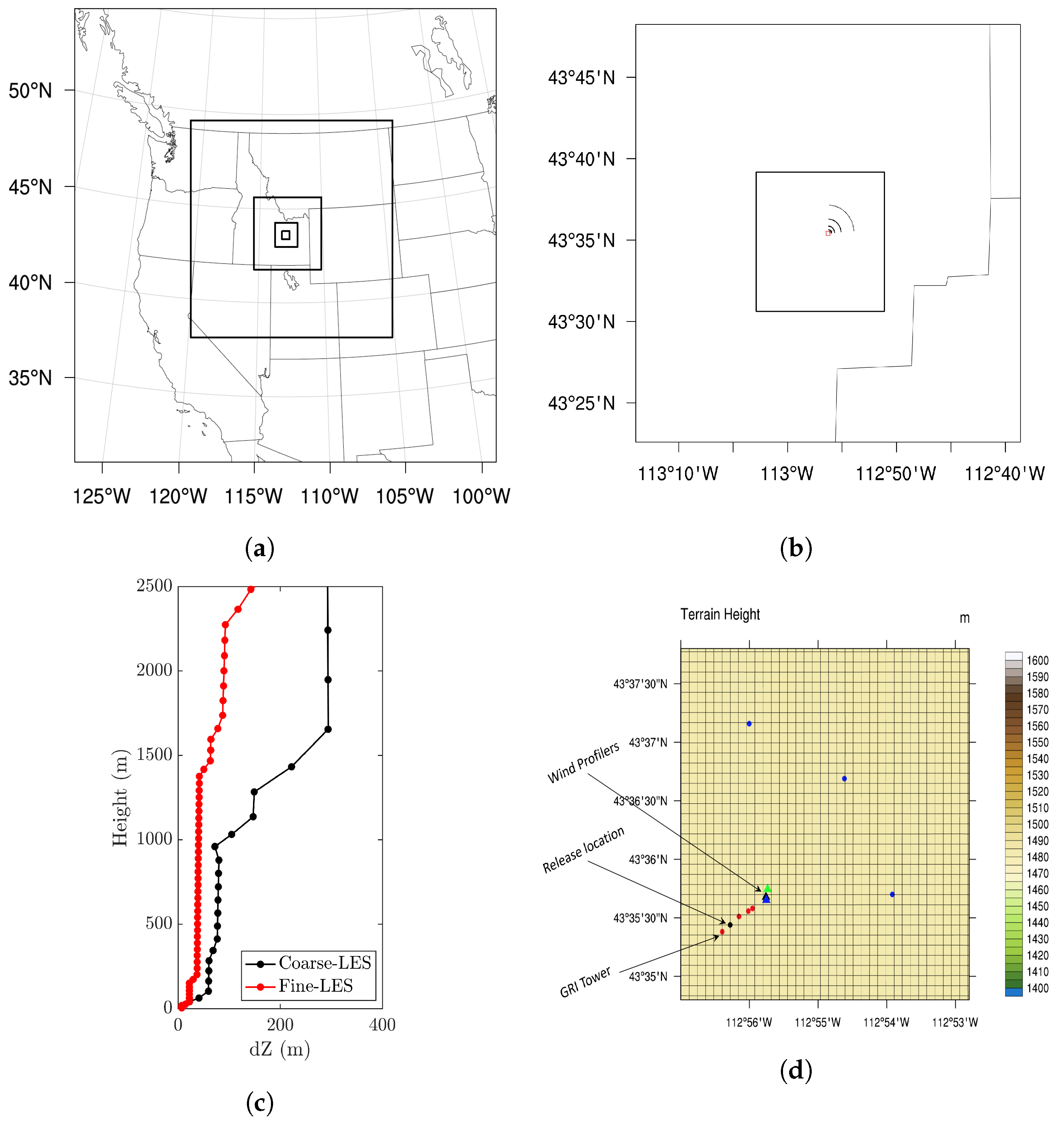
The Advanced Research version of WRF model (version 3.9.1) was configured with multiple nested domains as shown in Figure 1a,b. Domains D01, D02, D03 and D04 were nested with feedback turned “on” and were used for mesoscale simulations. Domains D05 and D06 were used for LES runs. The horizontal resolution for the mesoscale domains was 24.38 km (D01), 12.15 km (D02), 4.05 km (D03), 1.35 km (D04) and for LES domains was 450 m (D05) and 150 m (D06). The model top was considered at 100 hPa. Two vertical resolution configurations were used in the study; Figure 1c shows the vertical resolution changes in the first 2500 m. The coarser-in-vertical-LES simulations have a total of 69 levels with 22 levels inside the ABL. The finer-in-vertical-LES have a total of 99 levels with 40 levels inside the ABL. The first grid point in both LESs is at 3.65 m above ground.

Table 1. WRF model configuration for mesoscale and LES domains.

	D01	D02	D03	D04	D05	D06
Horizontal grid size (km)	24.38	12.19	4.06	1.36	0.45	0.15
Grid Points	70 × 70	100 × 100
IBC	NARR/RAP/NAM				D04	D05
PBL Scheme	YSU/MYNN2.5/MYJ				None
Time Step (s)	27	9	3	1	1/6	1/16
Nesting	-	2-way			1-way

gives the summary of WRF model domains and respective physics options used. The output from the inner most mesoscale domain D04 was saved at a frequency of 10 min and was used as the initial and boundary conditions (IBC) for LES domain D05. The output from D05 LES was saved every 10 min and was used as IBC for the finer LES domain D06. The LES and mesoscale simulations were run separately, meaning there was no feedback from the LES domains to the mesoscale domains. All the mesoscale runs were initialized at midnight (00 MST) of the day before the actual IOP day and were run for a period of 24 h. Meteorological initial and boundary conditions for D01 were obtained from three different datasets provided by National Centers for Environmental Predictions (NCEP). The first dataset is North American Regional Reanalysis (NARR), which has a horizontal resolution of 32 km and were updated every 3 h. The second dataset is North American Mesoscale Forecast System Analyses (NAM), which has a horizontal resolution of 12 km and were updated every 6 h. The third and final dataset is Rapid Refresh Analyses (RAP) which has a horizontal resolution of 13.5 km and updated every 1 h. The intention of selecting these datasets was not only to see the performance of reanalysis/analysis products, but also to see the model performance when the IBCs were updated at different frequencies. Apart from the IBCs, various parameterization schemes can be selected inside WRF model to simulate the PBL dynamics.

Table 2. Combinations of WRF mesoscale simulations parameterizations included in the sensitivity analysis.

Case ID	IBC	PBL Scheme	Surface Layer Scheme	Microphysics Scheme	IOP Tested
Meso1	NARR	MYNN2.5	RMO	Kessler	IOP1
Meso2	NAM
Meso3	RAP
Meso4	NARR			M2M
Meso5	NAM
Meso6	RAP
Meso7	NARR		MOJ	M2M
Meso8	NARR		MYNN	M2M
Meso9	NARR	YSU	RMO	Kessler
Meso10	NAM
Meso11	RAP
Meso12	NARR			M2M
Meso13	NAM
Meso14	RAP
Meso15	NARR	MYJ	MOJ	M2M
Meso16	NARR	MYNN2.5	RMO	M2M	IOP2
Meso17			MOJ
Meso18			MYNN
Meso19		YSU	RMO
Meso20		MYJ	MOJ

gives the list of all cases simulated in this study to understand the sensitivity of WRF model for respective physics schemes. Simulations were prepared with combination of three PBL schemes (Yonsei University scheme-YSU, Mellor–Yamada–Janjic scheme-MYJ and Mellor–Yamada–Nakanishi–Niino 2.5 level scheme-MYNN2.5), three surface layer schemes (Revised MM5 Monin–Obukhov scheme-RMO, Monin–Obukhov–Janjic scheme-MOJ and Mellor–Yamada–Nakanishi–Niino scheme-MYNN) and two microphysics schemes (Morrison 2-Moment scheme-M2M and Kessler scheme-Kessler). Observational (also known as station) nudging and objective analysis (OA) were performed on the IBCs used for mesoscale domains (D01, D02 and D03) using the surface and sounding data from MADIS. Observational data from MADIS was obtained in little_r format and fed to OBSGRID, which generated the additional files required for observational nudging. No nudging was performed within PBL and surface levels, following the study of Gilliam et al. [25], who showed that surface nudging induced additional bias in wind speed during convective conditions. Ngan et al. [31] recently used dynamically-downscaled mesoscale WRF modeled meteorological fields during PSB1 to perform dispersion simulations in HYSPLIT [32].

3. Results

3.1. WRF Mesoscale Sensitivity Tests

The performance of WRF model subjected to different initial and boundary conditions was validated using three different datasets (Table 1). In addition, with each dataset, the three most commonly used different PBL schemes and two different microphysics schemes were used. The three PBL schemes tested were Yonsei University PBL scheme (YSU, [33]), Mellor–Yamada–Nakanishi–Niino 2.5 level scheme (MYNN2.5, [34]) and Mellor–Yamada–Janjic (MYJ, [35]). PBL schemes in WRF only work with certain Surface layer schemes. YSU scheme was used with Revised MM5 Monin–Obukhov scheme (RMO) and MYJ scheme was used with Monin–Obukhov–Janjic scheme (MOJ). MYNN2.5 PBL scheme can be used with multiple surface layer schemes. It was tested with RMO, MOJ and MYNN surface layer scheme. The main purpose of PBL scheme was to distribute the surface fluxes and to take care of the boundary layer growth. MYJ and MYNN2.5 PBL schemes estimate the boundary layer growth by Turbulent Kinetic Energy (TKE) prediction; these were treated as local schemes, whereas YSU PBL scheme is a non-local scheme, which estimates the PBL height based on the entrainment and mixing. The two microphysics schemes tested were Kessler ([36]) and Morrison 2-moment (M2M) ([37]). All sensitivity tests were performed on the mesoscale domains of IOP1. All parameterization combinations used for the sensitivity study are listed in Table 2. WRF mesoscale outputs from domain D04 were compared against the observations from the surface measurements made during PSB1. The statistical measures (definitions given in Appendix A), namely mean bias (MB, range = $-\infty$ to $+\infty$), root mean square error (RMSE, range = 0 to $+\infty$), index of agreement (IOA, range = 0 to 1) and mean absolute error (MAE, range = 0 to $+\infty$), were calculated over the period of IOPs (i.e., 2.5 h) for model’s performance. MB tells the overall bias of the model while MAE tells how close the model results were compared to the actual observations. RMSE tells the deviations of model errors and IOA gives a single value that can assess the capability of the model. The ideal value for MB, RMSE and MAE is 0, while for IOA is 1.

3.1.1. Surface Meteorological Variables

The 2-m temperature (T${}_{2m}$), 10-m horizontal wind speed (U${}_{10m}$) and direction (UDir${}_{10m}$) were calculated as diagnostic variables in WRF mesoscale simulations. The performance statistics of each mesoscale parameterization choice was tested using the metrics given in Equations (A1)–(A4) of Appendix A.

Table A1. Statistical measures for 2-m temperature in mesoscale simulations performed. Bold values represent the best values.

Case	T${}_{2\mathit{m}}$
	MB (${}^{\circ }$C)	RMSE (${}^{\circ }$C)	IOA	MAE (${}^{\circ }$C)
Meso1	−2.02	2.87	0.72	2.01
Meso2	−3.51	3.92	0.75	3.12
Meso3	−2.69	3.04	0.71	3.02
Meso4	−0.87	1.72	0.78	1.71
Meso5	−1.97	2.51	0.67	2.51
Meso6	−1.34	1.98	0.81	1.97
Meso7	−0.88	1.66	0.78	1.64
Meso8	−1.17	1.93	0.82	1.90
Meso9	−2.05	2.97	0.70	2.96
Meso10	−3.71	4.13	0.63	4.12
Meso11	−1.07	1.71	0.77	1.69
Meso12	−0.70	1.56	0.86	1.51
Meso13	−1.82	2.41	0.81	2.40
Meso14	−1.84	2.48	0.76	2.47
Meso15	−0.79	1.56	0.88	1.58
Meso16	−0.42	1.33	0.77	1.13
Meso17	−0.53	1.36	0.72	0.85
Meso18	−0.37	1.33	0.81	0.84
Meso19	−0.33	1.03	0.84	0.75
Meso20	−0.47	1.38	0.68	0.85

,

Table A2. Statistical measures for 10-m wind speed in mesoscale simulations performed. Bold values represent the best values.

Case	U${}_{10\mathit{m}}$
	MB (ms${}^{-1}$)	RMSE (ms${}^{-1}$)	IOA	MAE (ms${}^{-1}$)
Meso1	1.06	0.72	0.63	0.65
Meso2	0.79	0.78	0.65	0.71
Meso3	1.09	1.28	0.62	1.13
Meso4	0.30	0.63	0.57	0.60
Meso5	0.47	1.02	0.70	0.85
Meso6	0.27	0.85	0.67	0.72
Meso7	0.73	0.95	0.71	0.83
Meso8	0.30	0.71	0.79	0.61
Meso9	0.56	0.86	0.66	0.70
Meso10	0.42	0.80	0.74	0.65
Meso11	0.32	0.67	0.73	0.58
Meso12	0.22	0.63	0.82	0.48
Meso13	0.50	0.96	0.68	0.79
Meso14	0.33	0.84	0.81	0.72
Meso15	0.24	0.61	0.81	0.50
Meso16	0.38	0.87	0.79	0.73
Meso17	0.41	0.93	0.80	0.75
Meso18	0.36	0.85	0.83	0.72
Meso19	0.45	0.83	0.86	0.60
Meso20	0.31	1.26	0.83	0.62

and

Table A3. Statistical measures for 10-m wind direction in mesoscale simulations performed. Bold values represent the best values.

Case	UDir${}_{10\mathit{m}}$
	MB (${}^{\circ }$)	RMSE (${}^{\circ }$)	IOA	MAE (${}^{\circ }$)
Meso1	−23.56	40.52	0.69	31.58
Meso2	−30.56	44.05	0.58	37.52
Meso3	−37.34	50.99	0.57	43.97
Meso4	−18.38	59.30	0.72	30.15
Meso5	−33.12	66.70	0.63	48.75
Meso6	−41.69	53.66	0.68	43.35
Meso7	−28.06	48.77	0.71	36.15
Meso8	−17.96	35.61	0.75	31.93
Meso9	−24.66	52.35	0.71	39.58
Meso10	−22.63	47.35	0.73	36.85
Meso11	−24.60	42.84	0.60	41.39
Meso12	−14.52	31.54	0.76	28.38
Meso13	−25.49	53.38	0.63	43.55
Meso14	−36.06	51.82	0.60	47.27
Meso15	−16.81	34.50	0.78	30.03
Meso16	−29.22	28.95	0.73	27.21
Meso17	−23.48	33.68	0.76	31.52
Meso18	−24.48	26.26	0.80	26.09
Meso19	−26.51	25.64	0.83	25.20
Meso20	17.01	31.16	0.78	26.91

give the model performance for T${}_{2m}$, U${}_{10m}$ and UDir${}_{10m}$. The observed values were taken from the measurements at GRI Tower during PSB1 and WRF simulated values were taken as horizontally averaged over a grid size of 3 × 3 near the GRI Tower location in WRF model.

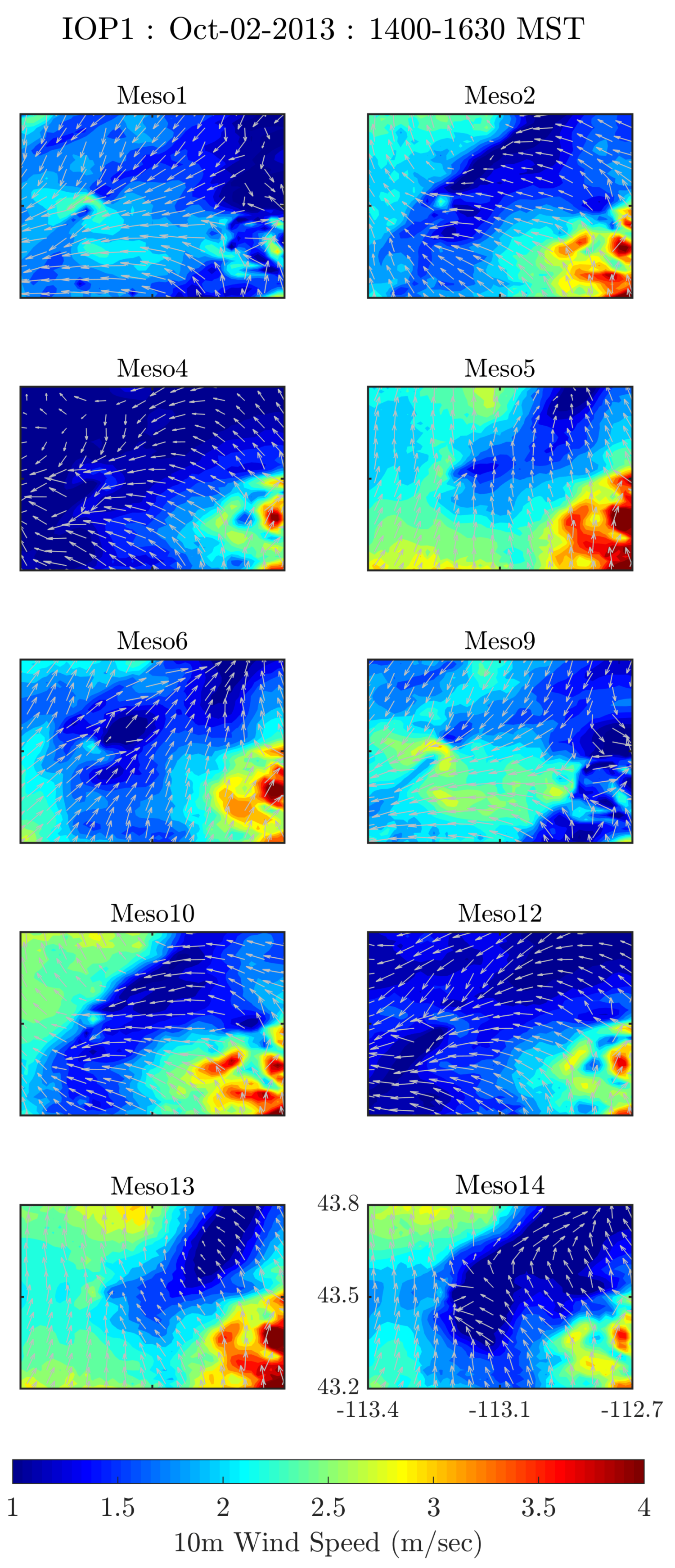
Of all combinations tested, the first 15 cases (i.e., Meso1–Meso15) were used to identify the model parameters that yield lowest errors during IOP1 and the last five were used to re-evaluate the schemes that performed best during the first 15 cases. The reason for this additional test was because of very low wind speeds during IOP1 while IOPs 2,4 and 5 have moderate wind speeds. In addition, wind directions during IOP1 were more dynamic and inhomogeneous in horizontal [29]. As shown in Table A1, Table A2 and Table A3, runs initialized with NARR dataset gave the least errors and highest index of agreement. Simulation Meso12 gave the lowest MB (−0.7 ${}^{\circ }$C), RMSE (1.56 ${}^{\circ }$C) and MAE (1.51 ${}^{\circ }$C) while Meso15 provided the lowest RMSE (1.56 ${}^{\circ }$C) and highest IOA (0.88) when 2-m temperatures were compared. All the WRF simulations (Meso1–Meso15 and Meso16–Meso20) underestimated the 2-m temperature, meaning that WRF model has cold-bias, which is consistent with other studies (e.g., [38,39]). For 10-m wind speeds, all parameterizations consistently overestimated the wind speed with Meso12 having the lowest MB (0.22-ms${}^{-1}$), MAE (0.48-ms${}^{-1}$) and highest IOA (0.82). Meso15 has the lowest RMSE (0.61-ms${}^{-1}$) for 10-m winds. For 10-m wind direction, Meso12 performed better with the lowest MB (−14.52${}^{\circ }$), MAE (28.38${}^{\circ }$) and RMSE (31.54${}^{\circ }$). Meso15 has the highest IOA (0.78). The most sensitive control variable in WRF simulations is the IBC dataset, after which PBL scheme gives the most variations in the results. Comparing simulations Meso1 with Meso4 or Meso9 with Meso12 showed that M2M microphysics scheme performed better keeping all other options the same. The effect of surface layer scheme is seen for mesoscale simulations during IOP2. Meso16, Meso17 and Meso18 were tested with same PBL scheme but with three different surface layer schemes (RMO, MOJ and MYNN). Out of the three surface layer schemes tested, MYNN PBL scheme performed best with MYNN surface layer scheme. The effect of PBL scheme was studied by comparing the simulations Meso8, Meso12 and Meso15. As shown in Table A1, Table A2 and Table A3, all three PBL schemes performed similarly, with either YSU scheme or MYJ scheme giving the lowest errors and highest index of agreement. This was observed for IOP2 simulations as well, where Meso18, Meso19 and Meso20 performed better than Meso16 and Meso17. The spatial distribution of wind speed across the domain was also dependent on the parameterization used. Figure 2 shows the 2.5-h time-averaged surface wind contours with wind direction barbs drawn at every other third grid point for selective meso cases during IOP1. Runs initialized with NAM datasets showed the most variability in 10-m wind speed across the domain, while runs initialized with NARR datasets showed the least variability. The wind directions differed largely based on the IBC used for meso runs. NAM runs have the wind blowing from the south. NARR runs have the winds blowing from the east and northeast. RAP runs have the 10-m winds blowing to the west and northwest.

3.1.2. PBL Heights

WRF simulated PBL heights were compared against the values observed from the radiosonde launches during IOP1 and IOP2. Radiosonde balloons were launched before the release of tracer and after the end of last sampling period [29]. Runs initialized with NARR dataset could simulate the PBL height reasonably as seen from Figure 3. The effects of other parameterizations such as surface layer scheme and microphysics scheme on the development of PBL height were not significant.

In all simulations, WRF model underestimated the PBL height with runs Meso7, Meso8, Meso12 and Meso15 giving the difference of around 200 m with the observed PBL height. The highest difference of >600 m was observed in PBL height for simulations with YSU PBL scheme and Kessler microphysics scheme (Figure 3a). During IOP2 (Figure 3b), the difference in PBL height was around 150–200 m for all simulations (Meso16–Meso20).

3.1.3. Meteorological Conditions without Nudging

To know the effect of OA, five simulations were performed without nudging the boundary conditions. The cases selected for these simulations were Meso4, Meso7, Meso8, Meso12 and Meso15 as they were initialized with NARR dataset and used M2M micro-physiscs scheme, which gave better performance, as shown in Table A1, Table A2 and Table A3 and Figure 3. The performance metrics presented in Section 3.1.3 were used to estimate the model performance for cases with no nudging performed and the results are presented in

Table A4. Statistical measures for 2-m temperature in mesoscale simulations performed without nudging.

Case	UDir${}_{10\mathit{m}}$
	MB (${}^{\circ }$)	RMSE (${}^{\circ }$)	IOA	MAE (${}^{\circ }$)
Meso4-No-OA	−1.69	2.13	0.72	2.10
Meso7-No-OA	−1.28	1.82	0.73	1.91
Meso8-No-OA	−1.73	2.21	0.76	2.11
Meso12-No-OA	−1.17	1.91	0.80	1.70
Meso15-No-OA	−0.85	1.92	0.79	1.88

,

Table A5. Statistical measures for 10-m wind speed in mesoscale simulations performed without nudging.

Case	UDir${}_{10\mathit{m}}$
	MB (${}^{\circ }$)	RMSE (${}^{\circ }$)	IOA	MAE (${}^{\circ }$)
Meso4-No-OA	0.37	0.78	0.48	0.74
Meso7-No-OA	0.92	1.15	0.64	0.91
Meso8-No-OA	0.39	0.92	0.71	0.42
Meso12-No-OA	0.31	0.72	0.76	0.65
Meso15-No-OA	0.33	0.82	0.75	0.72

and

Table A6. Statistical measures for 10-m wind direction in mesoscale simulations performed without nudging.

Case	UDir${}_{10\mathit{m}}$
	MB (${}^{\circ }$)	RMSE (${}^{\circ }$)	IOA	MAE (${}^{\circ }$)
Meso4-No-OA	−30.81	71.32	0.65	41.70
Meso7-No-OA	−40.72	61.25	0.56	51.42
Meso8-No-OA	−28.57	46.72	0.59	41.51
Meso12-No-OA	−30.33	41.82	0.68	39.84
Meso15-No-OA	−35.07	50.12	0.63	43.29

. Overall, the model performance improved in terms of increase in IOA, and decrease in MB, RMSE and MAE, as shown in Table A1, Table A2, Table A3, Table A4, Table A5 and Table A6. OA improved the IOA by 7–11% for T${}_{2m}$, 8–15% for U${}_{10m}$, and 11–19% for UDir${}_{10m}$. Similar improvements in IOA for temperature and wind speed, after performing OA, were observed by Li et al. [28] who simulated the meteorological conditions during the 2013 Deriving Information on Surface conditions from Column and Vertically Resolved Observations Relevant to Air Quality Texas campaign; and by Ngan et al. [24] who simulated the meteorological conditions during the Air Quality Study campaign in Texas in 2006. In addition, the PBL height predictions improved (not shown) for the nudged cases especially towards the end of IOP. Based on these results and from the studies mentioned above, performing OA is recommended to improve model performance especially if the model fields are intended to be used for studies, such as transport and dispersion.

Following the sensitivity analysis of surface meteorological variables and PBL height, Meso12 and Meso15 were considered as the best ensemble of WRF parameterizations. Subsequent LES runs made in this study were based on the boundary conditions from mesoscale parameterizations used in Meso12 case.

3.2. LES Simulation Results

After finalizing the mesoscale parameterizations, mesoscale simulations were carried out for remaining IOPs 4 and 5. LES runs were initialized 2 h before the actual tracer release during individual IOPs and the simulations were run for 6 h. Thus, IOP1 was initialized at 1200 MST, while IOPs 2 and 5 were initialized at 1030 MST and IOP4 was initialized at 1130 MST. Two sensitivity tests were performed on the innermost LES domain. The first test varied the vertical resolution of the model for IOPs 1,2 and 4. The second test was conducted for IOP5 to see the effect of SGS models used in WRF-LES.

3.2.1. Effect of Vertical Resolution

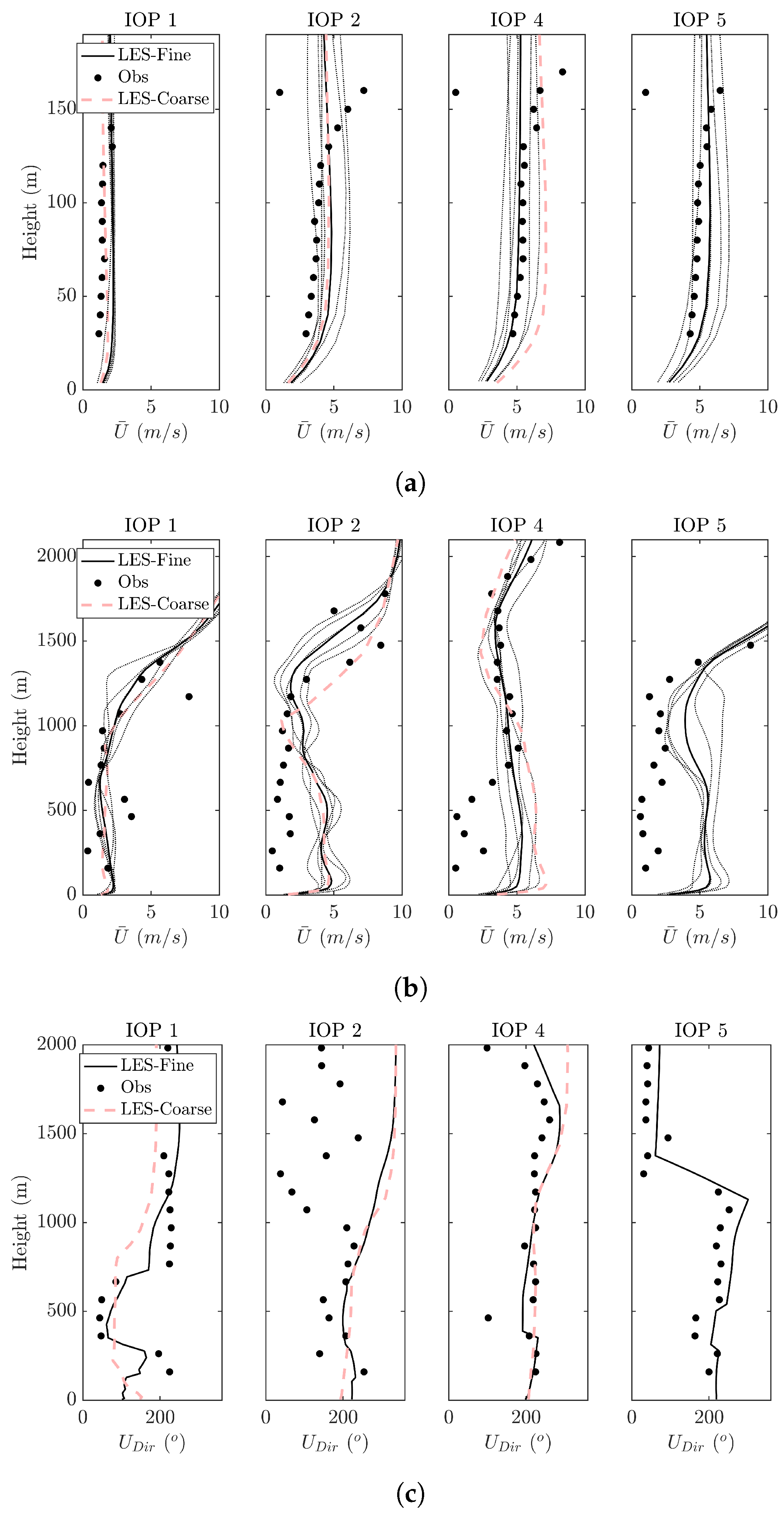
The ability of WRF model to accurately predict the profiles inside the CBL depends on the vertical resolution and number of levels inside the boundary layer [11]. Thus, two vertical resolutions were tested in this study for the LES runs during IOPs 1, 2 and 4. The Coarser-LES has a total of 69 levels in the tropopause with 22 levels below 1300 m. The fine-LES had a total of 99 levels with 40 levels below 1300 m. The first grid point in both coarse-LES and Fine-LES was at 3.65 m from ground. The vertical resolution change with height and the difference between coarse-LES and fine-LES vertical resolution is shown in Figure 1c. Vertical profiles of 2.5-h time-averaged horizontal wind speed from coarse- and fine-LES were compared against the measured profiles from Atmospheric Research and Technology (ART) Radio Acoustic Sounding System (RASS) wind profiler and Atmospheric Systems Corporation (ASC) SOnic Detection And Ranging (SODAR) located inside the tracer sampling network. Figure 4a,b shows the comparison between the horizontal wind speed profile from coarse and fine-LES runs with that of measured profiles from SODAR and RASS profiler. As shown in Figure 4a, the effect of vertical resolution is minimum during IOP1 and IOP2, while the coarse-LES winds during IOP4 are larger than the fine-LES winds. Both coarse- and fine-LES were unable to capture the subtle shear observed between 125 m to 160 m. In addition, there is a discrepancy among the SODAR and RASS profiler readings near 160 m. For all IOPs, the first level measurement of RASS profiler at 160 m was significantly less than the SODAR readings at almost the same height. This was attributed to the fact that RASS profiler readings less than 5 ms${}^{-1}$ are suspect [29]. Figure 4c shows the comparison between the wind directions simulated by coarse- and fine-LES and measured values from RASS profiler. Although RASS profiler wind speed values are suspect below 5 ms${}^{-1}$, the wind directions measured by RASS were in general agreement with those measured by other sensors like SODAR. Wind direction results varied significantly based on the vertical resolution for IOP1 (Figure 4). This difference, although small, exists in IOP2 and IOP4. As shown in Figure 4c, wind direction change near 200 m and again at 700 m during IOP1 was well captured by LES. During IOP2, observed wind directions from RASS profiler were poorly organized above 1000 m, while the LES simulated winds were nearly constant.

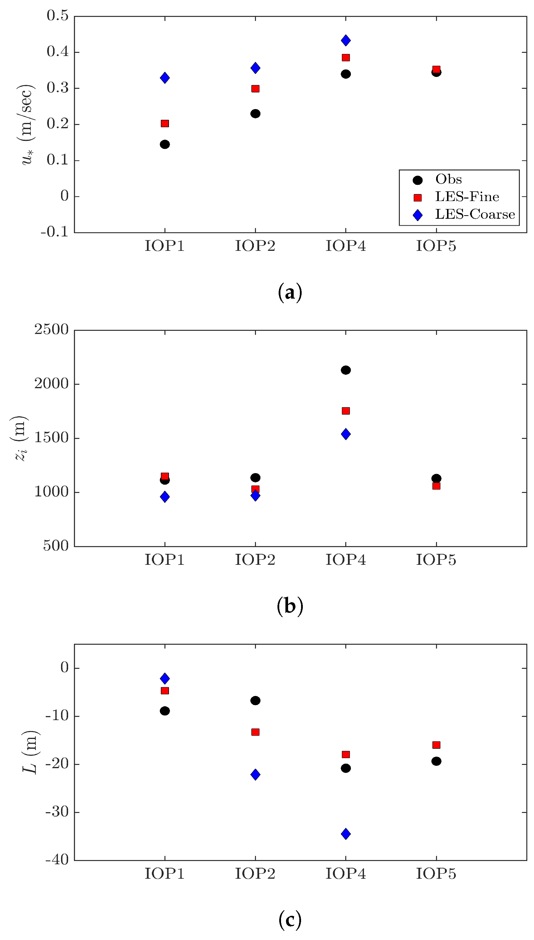
To know the effect of vertical resolution, friction velocity ($u_{\ast }$), planetary boundary layer height ($z_i$) and Monin–Obukhov length (L) were calculated and compared against the observed values (Figure 5). “$z_i$ observed” was estimated as the average between the values obtained from the two radiosonde launches, one before the tracer release and another after the tracer release, during each experiment [29]. “$z_i$ simulated” was estimated as the location of maximum vertical gradient of potential temperature [40]. $u_{\ast }$ in WRF was estimated by the surface layer scheme as:

$$u_{\ast }=\frac{\kappa U}{ln\left(\frac{z}{z_0}\right)-{\psi }_m(\frac{z}{L},\frac{z_0}{L})}$$

(1)

where $\kappa$ is von-Karaman constant, U is the wind speed at the lowest model level, z is the height of the lowest model level, $z_0$ is the roughness height, and L is the Monin–Obukhov Length scale calculated as:

$$L=\frac{-{\rho }_a{c}_p{u}_{\ast }^{3}T}{\kappa g{Q}_o}$$

(2)

where ${\rho }_a,c_p,T$ are density, specific heat and surface temperature of air, g is the gravitational constant and $Q_o$ is the vertical heat flux. As shown in Figure 5, the difference among $u_{\ast }$, $z_i$ and L simulated was reduced in fine resolution LES.

3.2.2. Effect of SGS Mixing Parameters

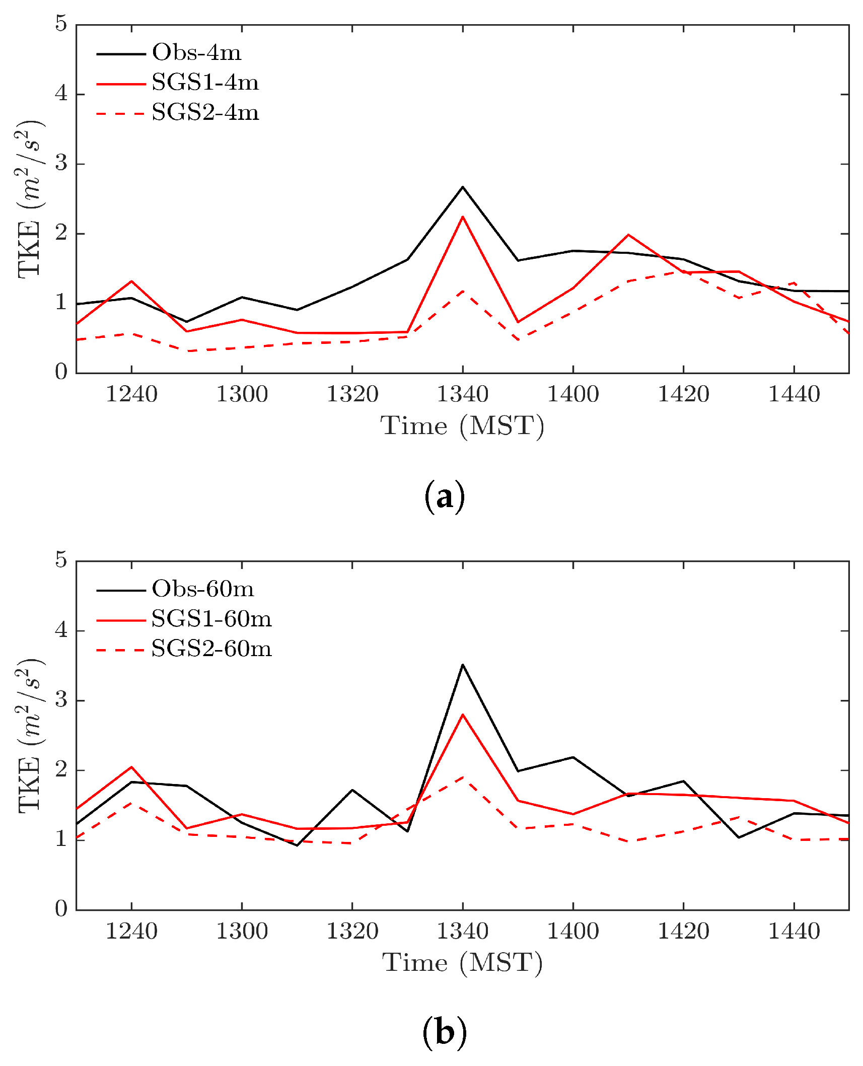
As mentioned above, the SGS model used in LES dictates the amount of turbulence that is resolved. WRF-LES has two eddy-viscosity based SGS models: a 3-D TKE-based model (SGS1) that uses a prognostic equation for TKE and a 3-D Smagorinsky model (SGS2) that uses the standard Smagorinsky approach. The SGS viscosity in WRF is dependent on a diffusion constant, which is related to the TKE coefficient ($c_k$) in SGS1 and Smagorinsky coefficient ($c_s$) in SGS2, respectively. Keeping in mind the limited computational resources, two additional cases were run for IOP5 with both SGS models using the default values for corresponding SGS coefficients (i.e., $c_k$ = 0.15 and $c_s$ = 0.25). Mirocha et al. [9] and Mirocha et al. [20] have showed that use of Non-linear Backscatter Analysis (NBA [41]) yields results for coarser LES runs that are similar to high resolution LESs. While NBA model accounts for momentum fluxes, SGS models in WRF provide the scalar fluxes. Although computationally expensive, NBA accounts for the reverse cascade of energy from smaller to larger eddies and thus is useful when running LES at resolutions greater than 100 m. Not many studies exist that have used NBA in real-world convective conditions with either of the SGS models in WRF. Green and Zhang [42] has used NBA for the first time to model the Hurricane Katrina, which includes both shear and buoyancy effects. They were able to simulate the turbulence structures at a resolution of 333.33 m. Recently, Mirocha et al. [43] has used the NBA accompanied by 3-D TKE SGS model to test the sensitivities of WRF-LES for idealized neutral and convective conditions. The 10-min time averaged TKE values observed at 4- and 60-m were compared against the two SGS models simulated in the study. Figure 6a,b shows the time variation of TKE evaluated at 3.65 and 62 m in LES. TKE from SGS2 run at 4 m was almost half of the observed value for most of the time (1230–1400 MST). TKE from SGS1 run was underestimated closer to the surface but was in good agreement at 60 m. The peak magnitude of TKE at 4 m (=2.67 m${}^2$s${}^{-2}$) and 60 m (=3.51 m${}^2$s${}^{-2}$) during IOP5 was observed around 1330–1340 MST. SGS1 model TKE at 4 m and 60 m for the 10-min average from 1330 to 1340 MST were 1.17 m${}^2$s${}^{-2}$ and 1.91 m${}^2$s${}^{-2}$, respectively. SGS2 model TKE at 4 m and 60 m for the 10-min average from 1330 to 1340 MST were 2.24 m${}^2$s${}^{-2}$ and 2.8 m${}^2$s${}^{-2}$, respectively. Overall, SGS1 performed better relative to SGS2.

3.2.3. Surface Meteorology

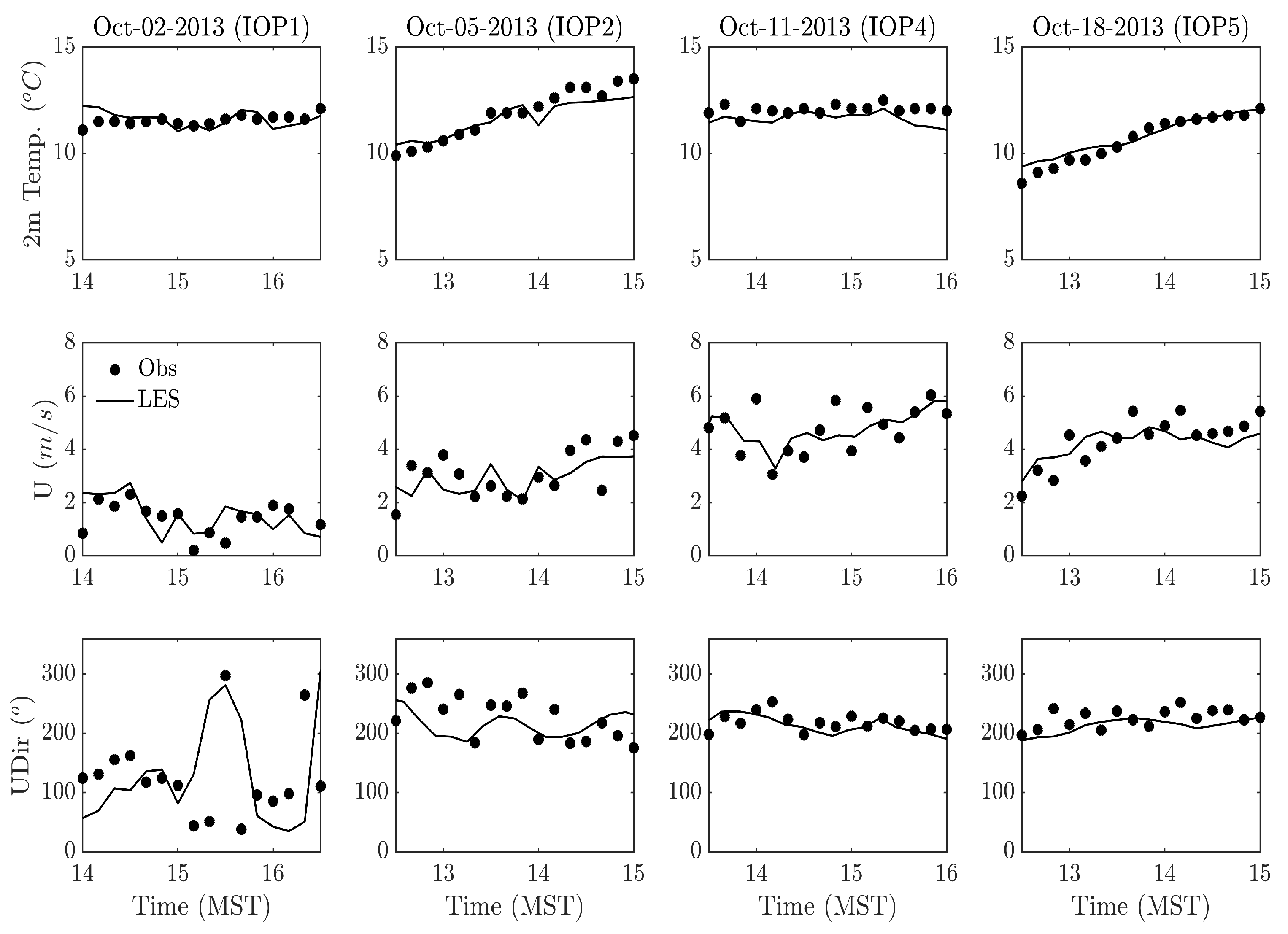
The 10-min averaged temperature at 2-m, horizontal wind speed and direction at 10-m near the GRI Tower were compared against the respective area averaged values from WRF-LES simulations. Figure 7 shows the temporal variation of the surface meteorological variables during the 2.5 h of individual IOPs conducted. IOP1 winds are low (<2 ms${}^{-1}$) and are not aligned in the direction of the tracer sampling network. WRF-LES was able to simulate the variations in wind speed and wind direction, especially from 1500 to 1600 MST during IOP1.

IOPs 2 and 5 have moderate winds with values ranging from 2-ms${}^{-1}$ to 4-ms${}^{-1}$ from both LES and measured values. LES underestimated the wind directions by 20${}^{\circ }$ during IOP2 but performed better during IOPs 4 and 5. There is no significant difference between the LES 2-m temperature and the observed values in all IOPs simulated. Figure 8 gives the wind rose comparison between the observed and LES simulated 15-m horizontal winds averaged over the Mesonet stations available within 16-km (≈10-mi) radius from the tracer release location. Distributed nature of wind directions during IOP1 shows the horizontal inhomogeneity [29], which was captured by the LES, although LES simulated winds were more towards south-southwest, while the observed wind directions were from southwest. In addition, the observed direction of maximum wind speed during IOP1 was from southwest, while the LES simulated the maximum winds from the east. Wind directions and magnitudes simulated in IOPs 2,4 and 5 were well captured by LES, as shown in Figure 7 and Figure 8.

3.2.4. Stability and Turbulence Statistics

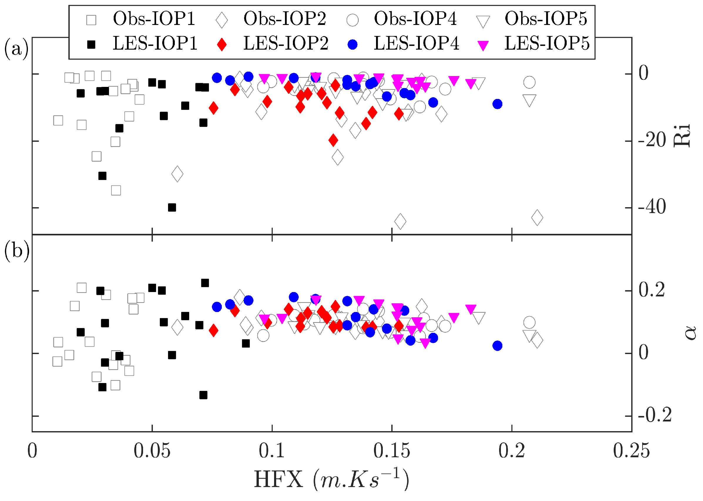
Atmospheric stability during PSB1 was estimated based on Richardson number ($Ri$) and shear exponent ($\alpha$) (estimated as in [19]) that were calculated from the 10-min averaged LES wind speed and temperatures at 8- and 60-m heights. $Ri$ evaluates the buoyant and shear tendencies inside the ABL making it a suitable parameter to estimate the stability. $Ri$ becomes 0 for neutral, >0 for stable and <0 for unstable atmosphere. In the case of highly unstable atmosphere, due to the strong mixing within the ABL, wind speed profiles are well-mixed making $\alpha$ very small. $Ri$ and $\alpha$ together gives the strength of unstable atmosphere. Figure 9 shows the comparison of $Ri$ and $\alpha$ between the LES simulations and observed values. For all IOPs simulated, $Ri$ was negative meaning that the atmosphere was unstable. $\alpha$ was used to further identify the degree of atmospheric instability. Stability during PSB1 varied from unstable to weakly unstable for IOPs considered in the study. $Ri$ during IOP1 and IOP2 varied between −0.5 and −40, while the values during IOP4 and IOP5 varied between −4 and −10. $\alpha$ during IOP1 varied greatly, from +0.2 to −0.2 while the values for remaining IOPs were between 0.2 and 0. Considering $Ri$ and $\alpha$ values, the stability during IOP1 and IOP2 was varied between unstable to weakly unstable, while for IOP4 and IOP5 the stability was consistently weakly unstable. Similar values of $\alpha$ were simulated in our previous study [19], where the shear and buoyancy dominated unstable atmosphere had $\alpha$ values ranging from 0.12 to 0.04. Shear-buoyancy convective conditions studied in [19] were similar to IOPs 4 and 5 in the present study. While IOPs 1 and 2 resemble the $\alpha$ values simulated for pure buoyant convective atmosphere, meaning the atmospheric stability was unstable to highly unstable. The stability criteria mentioned by us gave the same conclusions as Finn et al. [29] and Finn et al. [30] who used Pasquill–Gifford wind direction standard deviation method to estimate stability during PSB1.

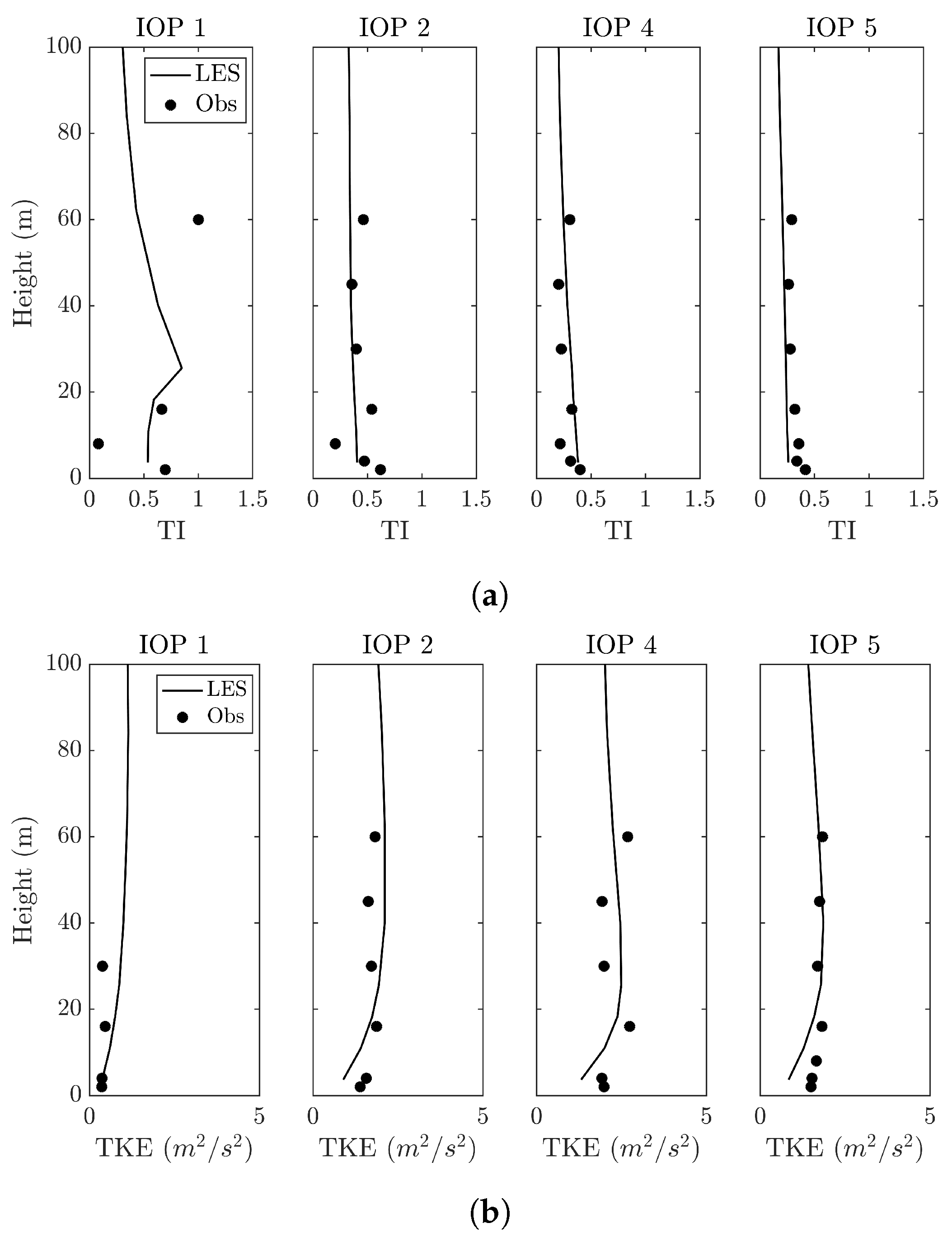
Figure 9 also shows the variations of surface sensible heat flux (HFX) during the IOPs. HFX during IOP1 was weak and varied from 0.06 to 0.01 mKs${}^{-1}$. HFX during IOPs 2, 4 and 5 was greater than IOP1 and varied between 0.06 to 0.2 mKs${}^{-1}$. Profiles of time averaged Turbulence Intensity ($TI={\sigma }_v/U$) and $TKE$ were evaluated at GRI tower location in LES and were compared against the observed values from 3D sonic-anemometers (Figure 10a,b). $TI$ from LES was almost constant from surface for IOPs 2, 4 and 5, while an increase in $TI$ at around 30-m was simulated during IOP1. During IOP1, at 60 m the $TI$ observed was greater than the near-surface values and was not captured by LES, meaning the modeled fluctuations in horizontal wind speed were underestimated. However, this was not the case during rest of the IOPs, where the $TI$ modeled was in good agreement with the observed values with a small difference near the surface. Similar to $TI$ (except for IOP1), $TKE$ profiles from the LES model were well mixed above 40 m. As shown in Figure 6, $TKE$ near the surface was underestimated by LES during IOPs 2, 4 and 5.

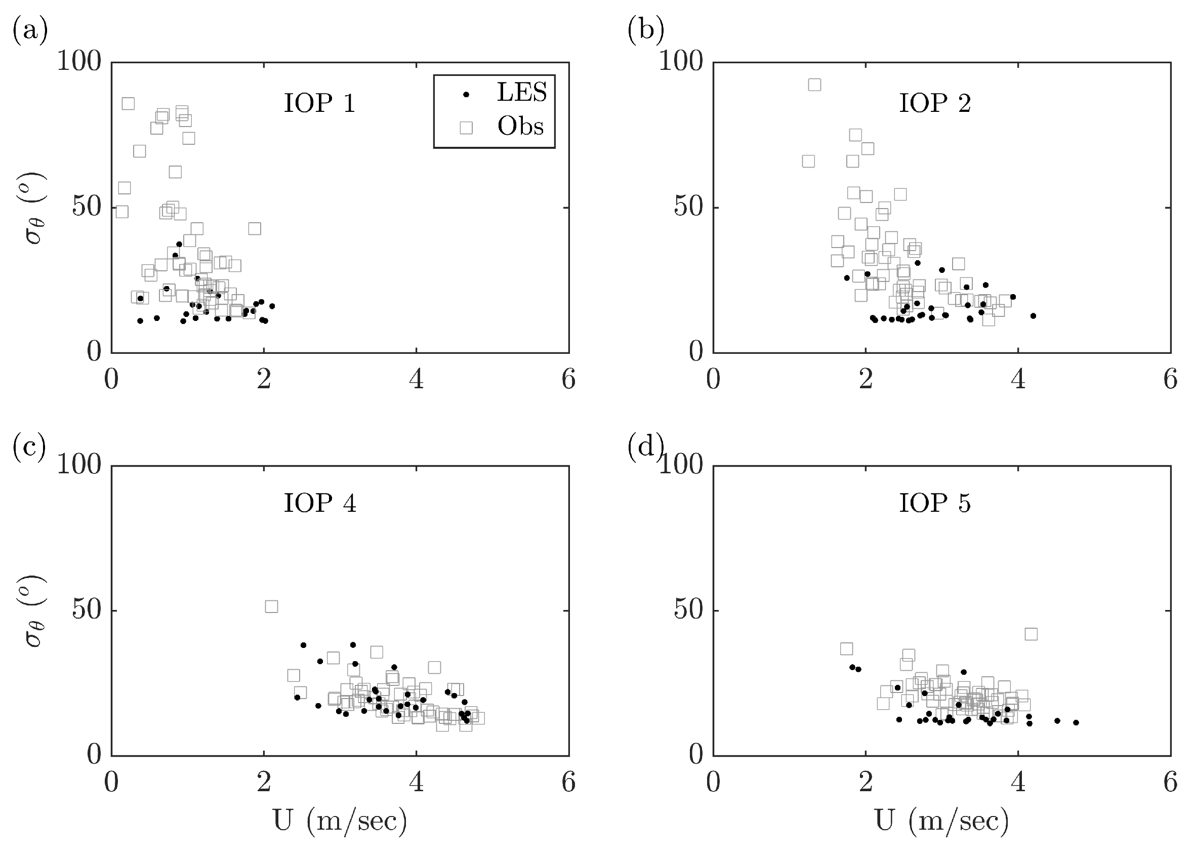
Standard deviations from the mean wind direction (${\sigma }_{\theta }$) are critical for dispersion applications as the horizontal spread of the pollutants or tracers depends on it [44]. Wind direction standard deviations estimated from 10-min averaged winds were compared against the observed values from GRI tower (Figure 11). Observed standard deviations during IOP1 and IOP2 were high compared to IOP4 and IOP5. LES simulated ${\sigma }_{\theta }$ were underestimated for wind speeds less than 3 ms${}^{-1}$, as shown in Figure 11a,b. For wind speed greater than 3 ms${}^{-1}$, as was the case during IOP4 and IOP5, LES simulated ${\sigma }_{\theta }$ were within the range of the observed values for IOP4 and were underestimated by approximately 10${}^{\circ }$ during IOP5.

3.2.5. Stability Parameter Scaling and Convective Features

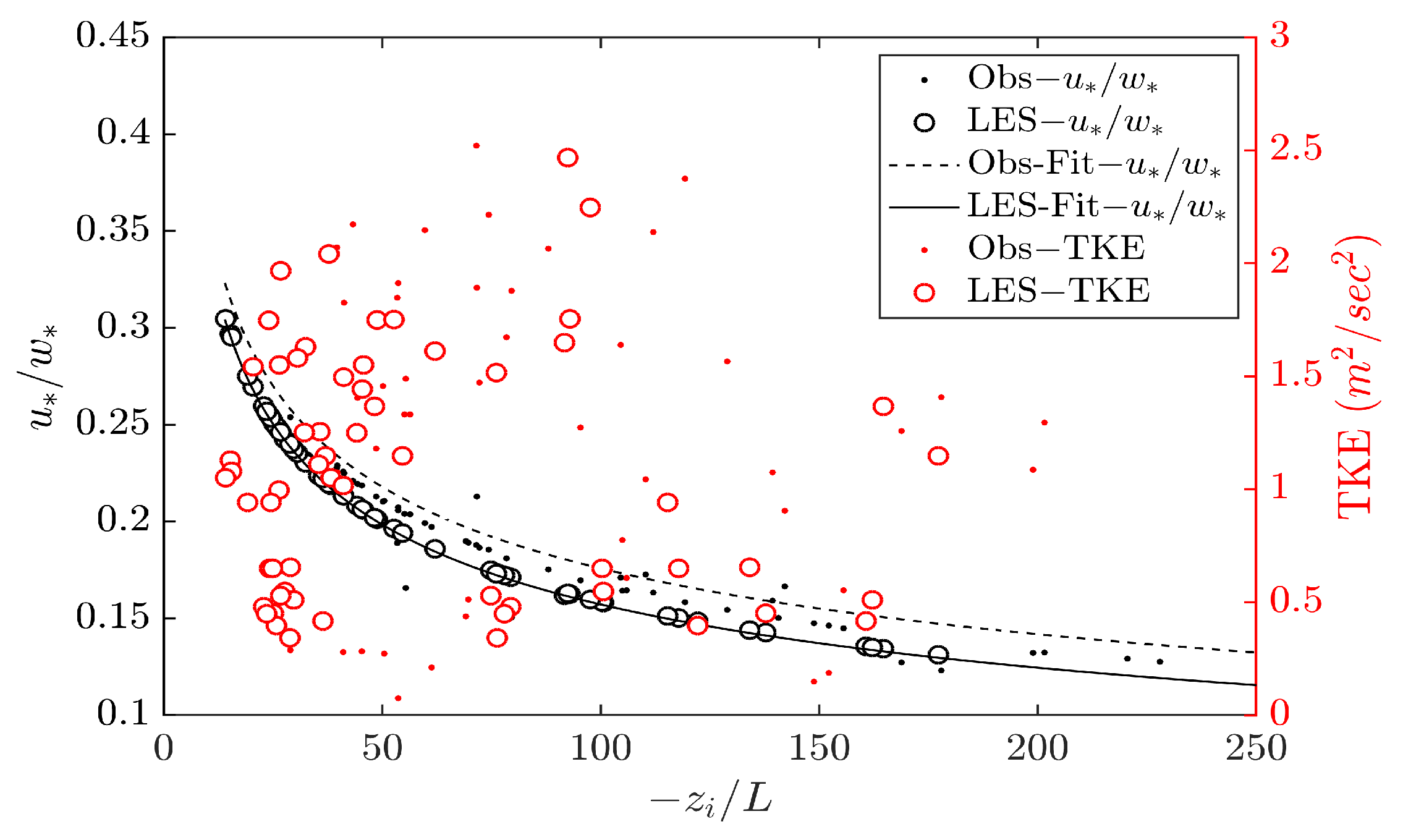
Monin and Obukhov [45] has developed a similarity theory in which the atmospheric stability can be determined by a non-dimensional stability parameter, $\zeta =z/L$. z is the vertical altitude above ground and L is the Monin–Obukhov length scale. The Obukhov length is positive for stable stratification, negative for unstable stratification and zero for neutral stratification. L represents the height beyond which buoyancy forces dominate the mechanical (shear) forces. The shear and buoyant productions of turbulent kinetic energy in the boundary layer can be compared from the ratio of friction velocity ($u_{\ast }$) to convective velocity scale ($w_{\ast }$ estimated as in [19]). Thus, the 10-min averaged turbulence velocity scale ratio ($u_{\ast }/w_{\ast }$) was studied against the stability parameter, as shown in Figure 12.

Both the observed and simulated data followed the scaling between the stability parameter and turbulence velocity scale ratio. There was little to no scatter in the data from the LES simulations, which can be attributed to the fact that the surface layer scheme used in WRF was the Revised Monin–Obukhov scheme. The 10-min averaged TKE was also studied against the stability parameter (Figure 12). While no scaling was observed between the TKE and stability parameter, the interplay between the buoyant and mechanical productions was in such a way that the total TKE (which is the sum of buoyant and mechanical productions) varied largely between 0.2 and 2.5 m${}^2$s${}^{-2}$. The fact that no scaling exists between TKE and stability parameter makes it impractical to use TKE alone for classifying the atmospheric stability. Wharton and Lundquist [46] have used TKE ranges together with parameters like $Ri$ and $\alpha$ to identify the atmospheric stability and to further classify the unstable atmospheric conditions. From TKE values observed at 80 m, Wharton and Lundquist [46] have proposed that moderately unstable conditions were characterized by TKE in the range of 1.0–1.4 m${}^2$s${}^{-2}$, and strongly unstable conditions exists when TKE >1.4-m${}^2$s${}^{-2}$. The 10-min averaged TKE values observed during IOP1 of PSB1 and respective LES simulated values were less than 0.5-m${}^2$s${}^{-2}$, yet the atmospheric state for IOP1 was characterized earlier as unstable based on Ri and values, as discussed in Section 3.2.1. Finn et al. [29] also concluded that the stability during IOP1 was unstable based on values observed. TKE values for remaining IOPs were in the range of 0.8–2.5 m${}^2$s${}^{-2}$. The stability classification discussed for IOPs 2-,4- and 5 in this study is in good agreement with that of Finn et al. [29], but contradicts the stability classification in [46]. One possible reason for this difference could be that the study area considered in [46] has an elevation of near-sea level with rolling-grassland type land cover and experiences some marine boundary layer influences, whereas the study region for PSB1 has an elevation of approximately 1500 m above sea-level with most of the land covered with sagebrush and grass. Site characteristics such as that of PSB1 were present in the work of St Martin et al. [47], who studied the performance of wind turbines based on the atmospheric stability and turbulence conditions. The 74-m observed TKE values in [47] range from 1 to 15 m${}^2$s${}^{-2}$ and the authors classified the atmosphere as stable for TKE < 3.0 m${}^2$s${}^{-2}$. Based on these studies, TKE ranges that can be used to classify the atmospheric stability appear to be site-specific. Thus, using metrics such as $u_{\ast }/w_{\ast }$, $Ri$, $\alpha$ or $-z_i/L$ to understand the atmospheric stability increases the robustness of analysis.

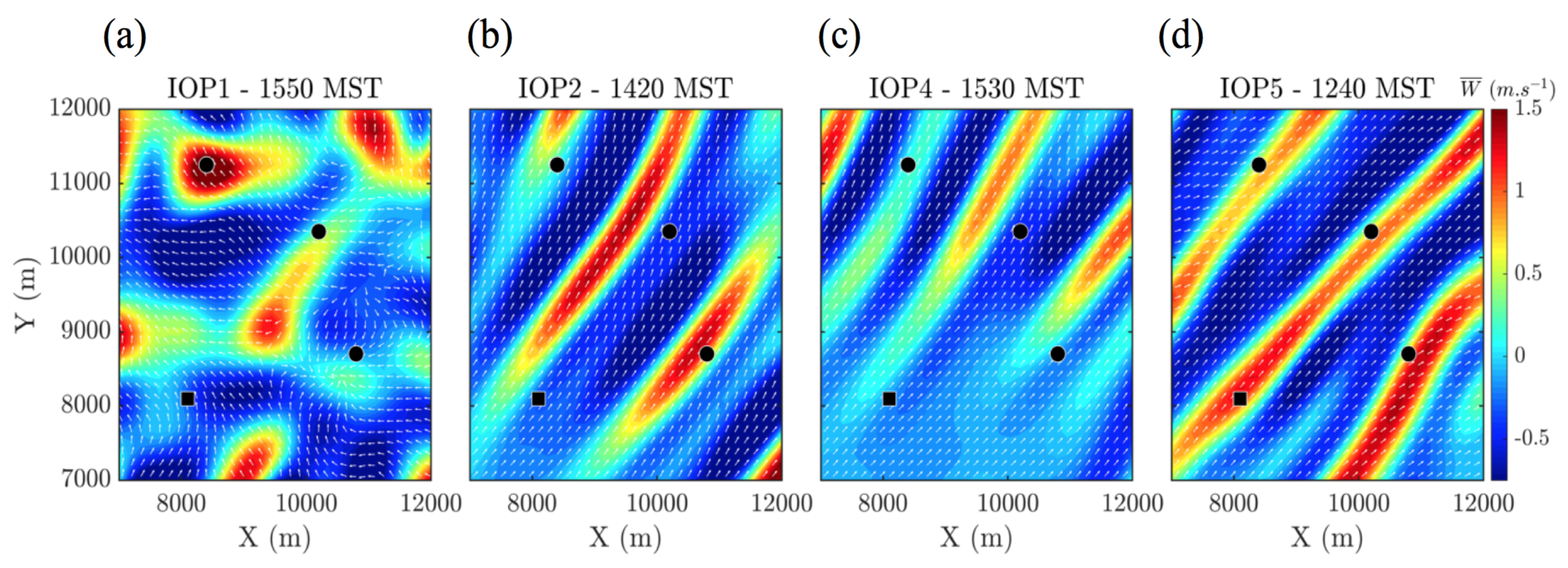
After evaluating the atmospheric stability in the boundary layer, knowledge of large-scale turbulent motions (organized convective features) will help in understanding the vertical transport of fluxes and scalars within the boundary layer [48]. In addition, presence of horizontally organized convective rolls may induce a meandering effect on plumes released in atmosphere [49,50,51]. Figure 13 shows the 10-min averaged vertical velocity contours overlapped with 10-min averaged wind vectors with wind speed normalized. The black square represents the release location and the black circles represent the 3-D sonic anemometers located at 3200-m arc radius during PSB1.

Studies (e.g., [49,52,53]) have shown that convective rolls can form in the boundary layer under combined conditions of moderate to strong sensible heat flux and winds. Such conditions were simulated during IOPs 2, 4 and 5 of PSB1. As shown in Figure 13b–d, organized roll-like structures were present at the study area of PSB1 during IOPs 2, 4 and 5, while convective cell type structures were present during PSB1. These results are consistent with findings of Lemone [49] and LeMone et al. [54] and observations reported by Weckwerth et al. [55], who suggested that convective roll formation occurs with the mean wind speed in the CBL greater than 3 ms${}^{-1}$, which was the case for the IOPs 2, 4 and 5 from the LES model. As for IOP1, larger stability parameter and low wind speeds in the CBL did not favor the formation of roll features; instead, convective cell type structures were observed from the vertical velocity contours, as shown in Figure 13a.

4. Summary and Conclusions

ABL conditions during Sagebrush tracer experiment were simulated at LES spatial and temporal scales using dynamic downscaling methodology in WRF. Five nested-mesoscale domains with grid resolutions ranging from 24 km to 1.3 km and two nested-LES domains with grid resolutions of 450 m and 150 m were simulated. Further reduction of grid resolution was not deemed necessary as the region covered is mostly flatland and does not have any features that can impact the wind field. Output from the mesoscale simulations was used to drive the LES. Sensitivity of WRF model performance to the initial and lateral boundary conditions, physics schemes and sub-grid scale models was evaluated. Mesoscale simulations were conducted with multiple PBL schemes, microphysics and surface layer schemes (Table 2). Sensitivity analysis following the metrics explained in Section 3.1 showed that NARR dataset with YSU PBL scheme coupled with Revised Monin–Obukhov surface layer scheme and Morrison-2nd-moment microphysics performed best. Model performance was improved with nudging the boundary fields through OA. Significant improvement was observed in wind direction predictions after the nudging (Table A3).

Although there exists no “thumb-rule” to use either mesoscale or LES at “terra-incognita” resolutions, we used LES at a grid resolution of 450-m, thus the turbulence started building up before the finest LES domain of 150-m resolution. Two vertical resolutions were tested inside the LES domains. Wind speed and wind direction profiles were compared against the observed values from SODAR and RASS during PSB1. Having 44 levels inside the boundary layer improved the model performance, especially with wind direction profiles (Figure 4c). Two SGS models (3D TKE and Smagorinsky) with NBA turned “on” were tested inside the LES domains. Comparing the time variation of TKE near surface (4-m) and at 60-m with the observed values during 2.5-h of PSB1 showed that both SGS models in WRF underestimated the TKE at 4-m. This might be avoided by using a dynamic sub-grid model, as suggested in previous studies [20].When using LES framework for dispersion applications, it is crucial to capture the mixing and stability conditions inside ABL. We compared the friction velocity, PBL height and Monin–Obukhov length against the measured values. Stability during the IOPs was estimated from Richardson number and shear exponent evaluated based on wind speed and temperatures between 4- and 60-m. IOPs 1 and 2 were unstable to weakly unstable, while IOPs 4 and 5 were consistently weakly unstable. Turbulence intensity and TKE profiles were well mixed 40-m above ground. Although rare, standard deviation of wind speed directions in the range of 70${}^{\circ }$–100${}^{\circ }$ were observed during IOPs 1 and 2 for wind speeds less than 3-ms${}^{-1}$ and in the range of 10${}^{\circ }$–40${}^{\circ }$ for IOPs 4 and 5. LES simulated wind direction standard deviations were underestimated for wind speeds less than 3-ms${}^{-1}$ and were in good agreement during IOPs 4 and 5. Wang and Jin [56] also observed the not-so-satisfactory performance of WRF model for wind speeds smaller than 2.5-ms${}^{-1}$ in their mesoscale runs.

In summary, this study shows the use of multiple nested domains to downscale the real boundary conditions from mesoscale resolutions to LES scales. A detailed description of ABL conditions during Sagebrush tracer experiment are given including the parameters that are critical for tracer dispersion studies. With proper selection of parameterizations, WRF model can be used to deliver the necessary initial and boundary conditions required for LES runs. Future study will be performed to validate the tracer dispersion properties from the experiments using the meteorological fields obtained from the ABL simulations.

References

1. Deardorff, J.W. Preliminary results from numerical integrations of the unstable planetary boundary layer. J. Atmos. Sci. 1970, 27, 1209–1211. [Google Scholar] [CrossRef]
2. Deardorff, J.W. Numerical investigation of neutral and unstable planetary boundary layers. J. Atmos. Sci. 1972, 29, 91–115. [Google Scholar] [CrossRef]
3. Deardorff, J.W. Three-dimensional numerical study of turbulence in an entraining mixed layer. Bound.-Layer Meteorol. 1974, 7, 199–226. [Google Scholar] [CrossRef]
4. Deardorff, J.W. Stratocumulus-capped mixed layers derived from a three-dimensional model. Bound.-Layer Meteorol. 1980, 18, 495–527. [Google Scholar] [CrossRef]
5. Moeng, C.H. A large-eddy-simulation model for the study of planetary boundary-layer turbulence. J. Atmos. Sci. 1984, 41, 2052–2062. [Google Scholar] [CrossRef]
6. Nieuwstadt, F.T.; Mason, P.J.; Moeng, C.H.; Schumann, U. Large-eddy simulation of the convective boundary layer: A comparison of four computer codes. In Turbulent Shear Flows 8; Springer: Berlin, Germany, 1993; pp. 343–367. [Google Scholar]
7. Moeng, C.; Dudhia, J.; Klemp, J.; Sullivan, P. Examining two-way grid nesting for large eddy simulation of the PBL using the WRF model. Mon. Weather Rev. 2007, 135, 2295–2311. [Google Scholar] [CrossRef]
8. Skamarock, W.C.; Klemp, J.B. A time-split nonhydrostatic atmospheric model for weather research and forecasting applications. J. Computat. Phys. 2008, 227, 3465–3485. [Google Scholar] [CrossRef]
9. Mirocha, J.; Lundquist, J.; Kosović, B. Implementation of a nonlinear subfilter turbulence stress model for large-eddy simulation in the Advanced Research WRF model. Mon. Weather Rev. 2010, 138, 4212–4228. [Google Scholar] [CrossRef]
10. Kirkil, G.; Mirocha, J.; Bou-Zeid, E.; Chow, F.K.; Kosović, B. Implementation and evaluation of dynamic subfilter-scale stress models for large-eddy simulation using WRF. Mon. Weather Rev. 2012, 140, 266–284. [Google Scholar] [CrossRef]
11. Talbot, C.; Bou-Zeid, E.; Smith, J. Nested mesoscale large-eddy simulations with WRF: Performance in real test cases. J. Hydrometeorol. 2012, 13, 1421–1441. [Google Scholar] [CrossRef]
12. Chu, X.; Xue, L.; Geerts, B.; Rasmussen, R.; Breed, D. A case study of radar observations and WRF LES simulations of the impact of ground-based glaciogenic seeding on orographic clouds and precipitation. Part I: Observations and model validations. J. Appl. Meteorol. Climatol. 2014, 53, 2264–2286. [Google Scholar] [CrossRef]
13. Cuchiara, G.; Rappenglück, B. Performance analysis of WRF and LES in describing the evolution and structure of the planetary boundary layer. Environ. Fluid Mech. 2018, 18, 1257–1273. [Google Scholar] [CrossRef]
14. Liu, Y.; Warner, T.; Liu, Y.; Vincent, C.; Wu, W.; Mahoney, B.; Swerdlin, S.; Parks, K.; Boehnert, J. Simultaneous nested modeling from the synoptic scale to the LES scale for wind energy applications. J. Wind Eng. Ind. Aerodyn. 2011, 99, 308–319. [Google Scholar] [CrossRef] [Green Version]
15. Ito, J.; Niino, H.; Nakanishi, M.; Moeng, C.H. An extension of the Mellor–Yamada model to the terra incognita zone for dry convective mixed layers in the free convection regime. Bound.-Layer Meteorol. 2015, 157, 23–43. [Google Scholar] [CrossRef]
16. Shin, H.H.; Hong, S.Y. Representation of the subgrid-scale turbulent transport in convective boundary layers at gray-zone resolutions. Mon. Weather Rev. 2015, 143, 250–271. [Google Scholar] [CrossRef]
17. Wyngaard, J.C. Toward numerical modeling in the “Terra Incognita”. J. Atmos. Sci. 2004, 61, 1816–1826. [Google Scholar] [CrossRef]
18. Bhaganagar, K.; Bhimireddy, S.R. Assessment of the plume dispersion due to chemical attack on April 4, 2017, in Syria. Nat. Hazards 2017, 88, 1893–1901. [Google Scholar] [CrossRef]
19. Bhimireddy, S.R.; Bhaganagar, K. Short-term passive tracer plume dispersion in convective boundary layer using a high-resolution WRF-ARW model. Atmos. Pollut. Res. 2018, 99, 901–911. [Google Scholar] [CrossRef]
20. Mirocha, J.; Kosović, B.; Kirkil, G. Resolved turbulence characteristics in large-eddy simulations nested within mesoscale simulations using the Weather Research and Forecasting Model. Mon. Weather Rev. 2014, 142, 806–831. [Google Scholar] [CrossRef]
21. Deng, A.; Stauffer, D.; Gaudet, B.; Dudhia, J.; Hacker, J.; Bruyere, C.; Wu, W.; Vandenberghe, F.; Liu, Y.; Bourgeois, A. 1.9 Update on WRF-ARW End-to-End Multi-Scale FDDA System; WRF Users’ Workshop: Boulder, CO, USA, 2009. [Google Scholar]
22. Lo, J.C.F.; Yang, Z.L.; Pielke, R.A. Assessment of three dynamical climate downscaling methods using the Weather Research and Forecasting (WRF) model. J. Geophys. Res. Atmos. 2008, 113. [Google Scholar] [CrossRef] [Green Version]
23. Otte, T.L. The impact of nudging in the meteorological model for retrospective air quality simulations. Part I: Evaluation against national observation networks. J. Appl. Meteorol. Climatol. 2008, 47, 1853–1867. [Google Scholar] [CrossRef]
24. Ngan, F.; Byun, D.; Kim, H.; Lee, D.; Rappenglück, B.; Pour-Biazar, A. Performance assessment of retrospective meteorological inputs for use in air quality modeling during TexAQS 2006. Atmos. Environ. 2012, 54, 86–96. [Google Scholar] [CrossRef]
25. Gilliam, R.C.; Godowitch, J.M.; Rao, S.T. Improving the horizontal transport in the lower troposphere with four dimensional data assimilation. Atmos. Environ. 2012, 53, 186–201. [Google Scholar] [CrossRef]
26. Rogers, R.E.; Deng, A.; Stauffer, D.R.; Gaudet, B.J.; Jia, Y.; Soong, S.T.; Tanrikulu, S. Application of the Weather Research and Forecasting model for air quality modeling in the San Francisco Bay area. J. Appl. Meteorol. Climatol. 2013, 52, 1953–1973. [Google Scholar] [CrossRef]
27. Ngan, F.; Cohen, M.; Luke, W.; Ren, X.; Draxler, R. Meteorological modeling using the WRF-ARW model for Grand Bay intensive studies of atmospheric mercury. Atmosphere 2015, 6, 209–233. [Google Scholar] [CrossRef]
28. Li, X.; Choi, Y.; Czader, B.; Roy, A.; Kim, H.; Lefer, B.; Pan, S. The impact of observation nudging on simulated meteorology and ozone concentrations during DISCOVER-AQ 2013 Texas campaign. Atmos. Chem. Phys 2016, 16, 3127–3144. [Google Scholar] [CrossRef] [Green Version]
29. Finn, D.D.; Clawson, K.; Eckman, R.M.; Carter, R.G.; Rich, J.D.; Strong, T.W.; Beard, S.A.; Reese, B.R.; Davis, D.; Liu, H.; et al. Project Sagebrush Phase 1; Technical Report; Air Resource Laboratory: Idaho Falls, ID, USA, 2015.
30. Finn, D.; Clawson, K.; Eckman, R.; Liu, H.; Russell, E.; Gao, Z.; Brooks, S. Project Sagebrush: Revisiting the value of the horizontal plume spread parameter σ y. J. Appl. Meteorol. Climatol. 2016, 55, 1305–1322. [Google Scholar] [CrossRef]
31. Ngan, F.; Stein, A.; Finn, D.; Eckman, R. Dispersion simulations using HYSPLIT for the Sagebrush Tracer Experiment. Atmos. Environ. 2018, 186, 18–31. [Google Scholar] [CrossRef]
32. Stein, A.; Draxler, R.R.; Rolph, G.D.; Stunder, B.J.; Cohen, M.; Ngan, F. NOAA’s HYSPLIT atmospheric transport and dispersion modeling system. Bull. Am. Meteorol. Soc. 2015, 96, 2059–2077. [Google Scholar] [CrossRef]
33. Hong, S.Y.; Noh, Y.; Dudhia, J. A new vertical diffusion package with an explicit treatment of entrainment processes. Mon. Weather Rev. 2006, 134, 2318–2341. [Google Scholar] [CrossRef]
34. Nakanishi, M.; Niino, H. An improved Mellor–Yamada level-3 model with condensation physics: Its design and verification. Bound.-Layer Meteorol. 2004, 112, 1–31. [Google Scholar] [CrossRef]
35. Janić, Z.I. Nonsingular Implementation of the Mellor-Yamada Level 2.5 Scheme in the NCEP Meso Model; US Department of Commerce, National Oceanic and Atmospheric Administration, National Weather Service, National Centers for Environmental Prediction: Washington, DC, USA, 2001.
36. Kessler, E. On the continuity and distribution of water substance in atmospheric circulations. Atmos. Res. 1995, 38, 109–145. [Google Scholar] [CrossRef]
37. Morrison, H.; Thompson, G.; Tatarskii, V. Impact of cloud microphysics on the development of trailing stratiform precipitation in a simulated squall line: Comparison of one-and two-moment schemes. Mon. Weather Rev. 2009, 137, 991–1007. [Google Scholar] [CrossRef]
38. Hu, X.M.; Nielsen-Gammon, J.W.; Zhang, F. Evaluation of three planetary boundary layer schemes in the WRF model. J. Appl. Meteorol. Climatol. 2010, 49, 1831–1844. [Google Scholar] [CrossRef]
39. Banks, R.F.; Tiana-Alsina, J.; Rocadenbosch, F.; Baldasano, J.M. Performance evaluation of the boundary-layer height from lidar and the Weather Research and Forecasting model at an urban coastal site in the north-east Iberian Peninsula. Bound.-Layer Meteorol. 2015, 157, 265–292. [Google Scholar] [CrossRef]
40. Stull, R.B. An Introduction to Boundary Layer Meteorology; Springer Science & Business Media: Berlin, Germany, 2012; Volume 13. [Google Scholar]
41. Kosović, B. Subgrid-scale modelling for the large-eddy simulation of high-Reynolds-number boundary layers. J. Fluid Mech. 1997, 336, 151–182. [Google Scholar] [CrossRef]
42. Green, B.W.; Zhang, F. Numerical simulations of Hurricane Katrina (2005) in the turbulent gray zone. J. Adv. Model. Earth Syst. 2015, 7, 142–161. [Google Scholar] [CrossRef] [Green Version]
43. Mirocha, J.D.; Churchfield, M.J.; Muñoz Esparza, D.; Rai, R.K.; Feng, Y.; Kosović, B.; Haupt, S.E.; Brown, B.; Ennis, B.L.; Draxl, C.; et al. Large-eddy simulation sensitivities to variations of configuration and forcing parameters in canonical boundary-layer flows for wind energy applications. Wind Energy Sci. 2018, 3, 589–613. [Google Scholar] [CrossRef]
44. Irwin, J. Estimating plume dispersion-a recommended generalized scheme. In Proceedings of the 4th Symposium on Turbulence, Diffusion, and Air Pollution, Reno, NV, USA, 15–18 January 1979. [Google Scholar]
45. Monin, A.; Obukhov, A. Basic laws of turbulent mixing in the surface layer of the atmosphere. Contrib. Geophys. Inst. Acad. Sci. USSR 1954, 151, e187. [Google Scholar]
46. Wharton, S.; Lundquist, J.K. Atmospheric stability affects wind turbine power collection. Environ. Res. Lett. 2012, 7, 014005. [Google Scholar] [CrossRef] [Green Version]
47. St Martin, C.M.; Lundquist, J.K.; Clifton, A.; Poulos, G.S.; Schreck, S.J. Wind turbine power production and annual energy production depend on atmospheric stability and turbulence. Wind Energy Sci. (Online) 2016, 1. [Google Scholar] [CrossRef]
48. Etling, D.; Brown, R. Roll vortices in the planetary boundary layer: A review. Bound.-Layer Meteorol. 1993, 65, 215–248. [Google Scholar] [CrossRef]
49. Lemone, M.A. The structure and dynamics of horizontal roll vortices in the planetary boundary layer. J. Atmos. Sci. 1973, 30, 1077–1091. [Google Scholar] [CrossRef]
50. Miao, S.; Chen, F.; LeMone, M.A.; Tewari, M.; Li, Q.; Wang, Y. An observational and modeling study of characteristics of urban heat island and boundary layer structures in Beijing. J. Appl. Meteorol. Climatol. 2009, 48, 484–501. [Google Scholar] [CrossRef]
51. Sandeepan, B.; Rakesh, P.; Venkatesan, R. Numerical simulation of observed submesoscale plume meandering under nocturnal drainage flow. Atmos. Environ. 2013, 69, 29–36. [Google Scholar] [CrossRef]
52. Sykes, R.; Henn, D. Large-eddy simulation of turbulent sheared convection. J. Atmos. Sci. 1989, 46, 1106–1118. [Google Scholar] [CrossRef]
53. Kim, S.W.; Park, S.U.; Moeng, C.H. Entrainment processes in the convective boundary layer with varying wind shear. Bound.-Layer Meteorol. 2003, 108, 221–245. [Google Scholar] [CrossRef]
54. LeMone, M.A.; Chen, F.; Tewari, M.; Dudhia, J.; Geerts, B.; Miao, Q.; Coulter, R.L.; Grossman, R.L. Simulating the IHOP_2002 fair-weather CBL with the WRF-ARW–Noah modeling system. Part II: Structures from a few kilometers to 100 km across. Mon. Weather Rev. 2010, 138, 745–764. [Google Scholar] [CrossRef]
55. Weckwerth, T.M.; Wilson, J.W.; Wakimoto, R.M.; Crook, N.A. Horizontal convective rolls: Determining the environmental conditions supporting their existence and characteristics. Mon. Weather Rev. 1997, 125, 505–526. [Google Scholar] [CrossRef]
56. Wang, C.; Jin, S. Error features and their possible causes in simulated low-level winds by WRF at a wind farm. Wind Energy 2014, 17, 1315–1325. [Google Scholar] [CrossRef]
Figure 1. (a) Mesoscale simulation domains configured in WRF, the innermost domain is D05. (b) LES domains configured in WRF, the innermost domain is D06. The black arcs shown in innermost domain in (b) represent the SF 6 tracer sampling network and the red square represent the release location. (c) Vertical resolution of coarse and fine LES runs simulated in this study. (d) Part of domain D06 showing the locations of Wind profilers, Grid 3 Tower (GRI) and Release location during PSB1. The blue dots represent the 3D sonic anemometers used at a radial distance of 3200 m from release location.
Atmosphere 09 00505 g001
Figure 2. The 10-m horizontal wind speed contours over the domain D04 for selective mesoscale cases during IOP1. Gray arrows represent normalized wind vectors drawn at every other third grid point.
Atmosphere 09 00505 g002
Figure 3. PBL height simulated by WRF mesoscale runs during: (a) IOP1; and (b) IOP2. The observed values correspond to the mixing heights estimated from the radiosonde launches during IOP1 and IOP2.
Atmosphere 09 00505 g003
Figure 4. Horizontal Wind Speed profiles of 2.5-h time-averaged from coarse- (red-dash) and fine-LES (solid) runs compared against: the SODAR readings (a); and RASS wind profiler (b). (c) Wind direction profiles of 2.5-h time-averaged compared against the RASS wind profiler. The black dotted lines represent the 30-min averaged wind profiles.
Atmosphere 09 00505 g004
Figure 5. Comparison of 2.5-h averaged (a) friction velocity ( u ), (b) PBL height ( z i ), and (c) Monin–Obukhov length (L) between the observed values and values calculated from coarse- and fine-LES at GRI tower. The PBL height observed values were averaged from the before and after radiosonde balloon flights released during the experiments; for more information on Radiosonde launches refer to [29].
Atmosphere 09 00505 g005
Figure 6. The 10-min averaged (a) 4-m and (b) 60-m TKE calculated from LES run using 3D TKE SGS model (SGS1) and Smagorinsky SGS model (SGS2), compared against the 3D Sonic anemometer measurements.
Atmosphere 09 00505 g006
Figure 7. Variation of 2-m temperature (2m Temp, top row), 10-m wind speed (U, middle row) and direction (UDir, bottom row) during 2.5 h of individual IOPs of PSB1.
Atmosphere 09 00505 g007
Figure 8. Wind Rose comparison between (a) observed and (b) LES simulated 15-m wind directions. From left to right: IOP1, IOP2, IOP4 and IOP5.
Atmosphere 09 00505 g008
Figure 9. The 10-min averaged (a) Richardson number ( R i ) and (b) Shear exponent ( α ) calculated based on the wind and temperature readings at 8 and 60 m.
Atmosphere 09 00505 g009
Figure 10. The 2.5 h time averaged: (a) turbulence intensity profile up to 100 m; and (b) T K E profile up to 100 m during IOPs 1, 2, 4 and 5. Black dots represent the observed values from 3D sonic-anemometers positioned on the GRI tower during PSB1.
Atmosphere 09 00505 g010
Figure 11. Comparison of wind direction standard deviation with wind speed during: (a) IOP1; (b) IOP2; (c) IOP4; and (d) IOP5. White boxes represent the observed values from GRI and COC towers during PSB1 and black dots represents the LES values.
Atmosphere 09 00505 g011
Figure 12. Ratio of friction velocity and convective velocity (left axis, black) and TKE (right axis, red) plotted against the stability parameter for all IOPs simulated. Solid dots indicate observed values of (black) and (red). White circles indicate LES simulated (black) and TKE (red). Dashed line is the power law fit between and observed, solid line is the power law fit from LES data.
Atmosphere 09 00505 g012
Figure 13. The 10-min averaged vertical velocity contours at 0.5 z i during (from left): (a) IOP1; (b) IOP2; (c) IOP4; and (d) IOP5. Normalized wind vectors show the 10-min averaged wind direction across the PSB1 site. Start time for the 10-min average period is given on top of each sub-figure. Black square represents the tracer release location during PSB1 and the black circles represent the sonic anemometers on the 3200-m arc radius from release location.
Atmosphere 09 00505 g013