Article

Identifying Key Potential Source Areas for Ambient Methyl Mercaptan Pollution Based on Long-Term Environmental Monitoring Data in an Industrial Park

1
Department of Environmental Science and Engineering, Fudan University, Shanghai 200438, China
2
Big Data Institute for Carbon Emission and Environmental Pollution, Fudan University, Shanghai 200433, China
*
Author to whom correspondence should be addressed.
Atmosphere 2018, 9(12), 501; https://doi.org/10.3390/atmos9120501
Submission received: 22 October 2018 / Revised: 26 November 2018 / Accepted: 6 December 2018 / Published: 17 December 2018
(This article belongs to the Section Air Quality)

Abstract

:
Precise source identification for ambient pollution incidents in industrial parks were often difficult due to limited measurements. Source area analysis method was one of the applicable source identification methods, which could provide potential source areas under these circumstances. However, a source area usually covered several sources and the method was unable to identify the real one. This article introduces a case study on the statistical source identification of methyl mercaptan based on the long-term measurements, in 2014, in an industrial park. A procedure for statistical source area analysis was established, which contains independent pollution episode extraction, source area calculation scenario definition, meteorological data selection, and source area statistical analysis. A total of 414 violation records were detected by five monitors inside the park. Three kinds of calculation scenarios were found and, finally, three key source areas were revealed. The typical scenarios of source area calculations were described in detail. The characteristics of the statistical source areas for all pollution episodes were examined. Finally, the applicability of the method, as well as the source of uncertainties, was discussed. This study shows that more concentrated source areas can be identified through the statistical source area method if several excessive emission sources exist in an industrial park.

1. Introduction

Locating emission sources of an ambient pollution episode is a critical step for air pollution control. Back-calculation of source parameters based on ambient concentration monitoring is one of the popular methods for locating emission sources, and has attracted increasing attention from researchers and environmental protection authorities [1,2,3,4].
Measurements from a monitoring network with a proper scale are fundamental for precise back-calculation of source parameters. The required scale for a monitoring network depends on the number of unknown parameters. Increased monitoring sites might improve the obtained result. Penenko V et al. addressed the data from 10 monitors to obtain the probability distribution density function of radionuclide emission sources [5]; Rude et al. indicated that at least 4 monitors on the ground were necessary to evaluate source location and source strength of a constant ground source by means of the inverse framework method [6]; Cantelli et al. applied 25 monitors to retrieve 3 different pollution sources using the genetic algorithm inverse model (GAIM) successfully [1].
This article presents a case study on the backtracking of organic ambient pollution sources in a chemical industrial park. Concentration measurements were provided by the ambient air quality monitoring network. There were five monitoring stations inside, however, only 1–2 of them could observe abnormal measurements in an air pollution episode in general. Obviously, the scale of this monitoring network was insufficient for the precise backtracking of pollution sources like those in the literature. Taking the positioning of emission sources as an example, the obtained solution domain was infinite if no prior information was available, or only measurements from 1–2 stations were given. The results obtained from source area analysis method shows that a fan-shaped source area in the upper wind of the monitors could be determined based on measurements from one monitor [7], and the source area became narrower when measurements from two monitors were given. Significantly, source areas in the latter case were still not small enough to precisely detect the real source. Consequently, the backtracking of an ambient pollution incident was only able to determine the distribution of source location, rather than the precise source location in our study. We found that source areas from different pollution incidents in numerous cases might overlap under certain weather conditions. Such overlaps indicated that excessive emissions from a source might lead to concentration exceedances at different monitoring stations and different time. Therefore, we decided to examine source area characteristics for a series of pollution incidents during a long period and aimed to backtrack the potential emission source areas from violation records in a year.
Back-calculation methods in the literature were investigated to find a proper method for our case study. Many inverse methods have been reported in the literature for the determination of pollution source parameters, such as genetic algorithms [1,8,9], simulated annealing algorithms [2,10], pattern search method [11], least square method [4,12], and probability modeling methods, including Markov chain Monte Carlo [3,7], and Sequential Monte Carlo [13]. These algorithms were used to find an optimal result of unknown parameters by looping over their solution domain, although they were with heavy computational loads. Finally, the method for source area analysis proposed by Huang et al. was adopted in this study, due to the relatively higher computational efficiency compared with other methods [7]. In this method, solution domain for source location was gridded where the center of each grid was regarded as a hypothetical source position. After that, an inverse method was applied to the optimization of other source parameters.
The dispersion of pollutants played an important role in source area analysis. A dispersion model was needed to simulate concentration distributions of pollutants. There were many candidate models, such as the Gaussian dispersion model, Lagrangian stochastic model, and computational fluid dynamics (CFD) model. Gaussian dispersion models, especially Gaussian plume model [13,14,15] and Gaussian puff model [7,16] were widely used as the forward dispersion simulation of air pollutants. Najafi and Gilbert and Annunzio et al. employed the Lagrangian puff models as the forward models [17,18]. A CFD model was used by Chow et al. in [19] and Kovalets IV et al. in [20]. Each model has its applicable conditions. In this study, Gaussian puff model was adopted. In theory, the Gaussian puff model is not the most suitable model for simulating the dispersion of organic air pollutants, like methyl mercaptan, which is the subject of this study. Precise dispersion models, like CFD, are preferable for exquisite simulation of the airflow and pollutant dispersion under complex terrain or surface, which is universal in industrial parks [21]. Gaussian puff model was finally used as a forward model in this study for the following considerations. On one hand, Gaussian puff model is a simple diffusion model with more mature applications and more available input parameters. A host of detailed parameters and accurate modeling about underlying surface are required in high-resolution simulation. On the other hand, the use of precise models can also cause errors and it is uncertain whether high-resolution models are more accurate than Gaussian puff model in the absence of accurate information on prior information of source emission parameters and environmental conditions [22]. To sum up, the inversion method combining Gaussian puff model with source area analysis was selected in this study.
In fact, there are very few cases like the ones in this article in practice. Studies about local pollution source identification in industrial parks are not enough to build a mature method system, and more studies are still in process. However, this article presented the research process and results from real cases. A statistical source identification method was developed successfully based on long-term monitoring data and plenty of violation records, in an industrial park with a huge number and widespread distribution of potential sources and insufficient source information. Under such situations, the statistical source area analysis method provides a guide to more direct information for daily emission source control, and can be used as a preliminary screening approach for pollution sources in an industrial park. Source location analysis of methylene mercaptan pollution episodes in a chemical industrial park in 2014 were addressed. Concentrations and meteorological measurements were analyzed, first, to develop a procedure for identifying independent pollution episodes and calculation scenarios. Then, the method to back-calculate source location distribution, as mentioned above, was applied repeatedly to find the potential source area for each independent episode. Finally, source area frequencies were summarized for all independent episodes to see whether there is some key suspected source area with high frequencies. The current work is organized as follows. The background of this study was described in Section 2, including the characteristics of the long-term meteorological data and concentration observations. The specific procedure taken in this case study on the industrial source backtracking, as well as the method of source area analysis, were presented in Section 3. Results were displayed in three parts in Section 4. Firstly, the output of independent pollution episodes was summarized. Subsequently, the characteristics of the obtained source areas from typical independent pollution episodes were introduced. The comprehensive statistical results of the source area frequencies, along with some investigations, were analyzed on the third part. Finally, conclusions and discussions were given in Section 5.

2. Case Description

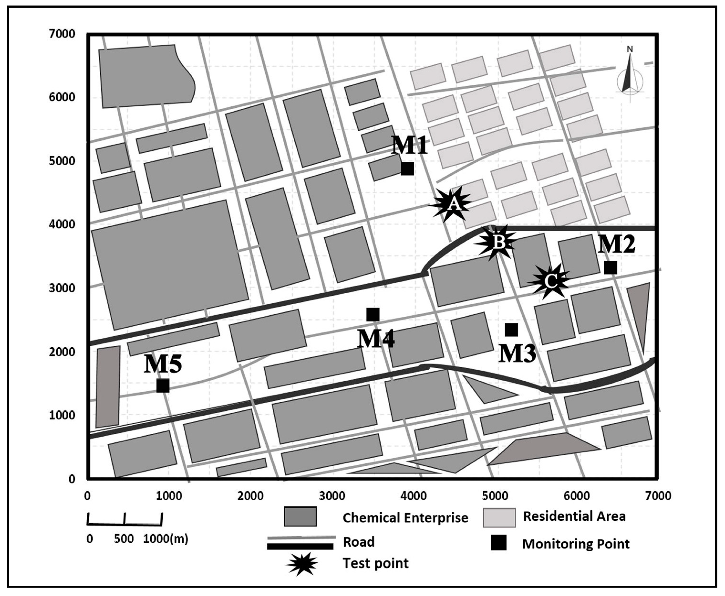
The studied case is a chemical industrial park about 22.5 km2 (Figure 1), in which there are lots of chemical industries specialized in petrochemicals, paints, inks, pigments, synthetic materials, medicines, pesticides, and several sewage treatments, etc. There are over 70 odor sources in this study region and there are few sources out of the study region. The source density in the northern part of this park was about 2–6 companies per square kilometer, while its southern counterpart was about 0.5–1.5 companies per square kilometer. Source heights range from 15 to 85 m. There are five fixed ambient air quality monitoring stations (M1–M5) and their surrounding conditions were described in 
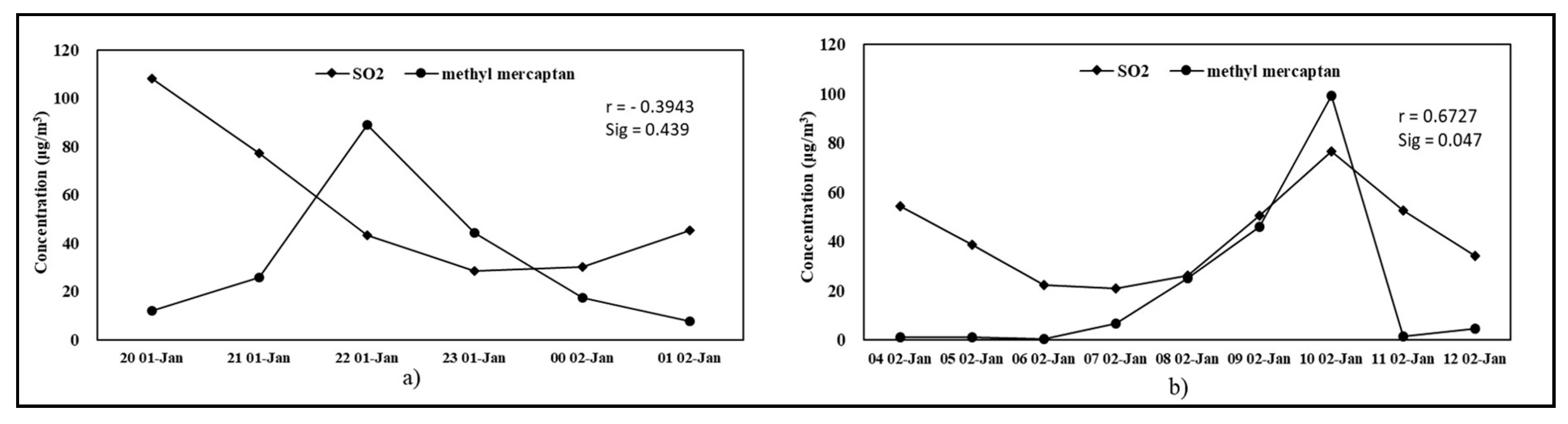
Table 1. Hourly measurements of wind and methyl mercaptan concentration, as well as SO2 concentration observations, in 2014, were collected in this study.
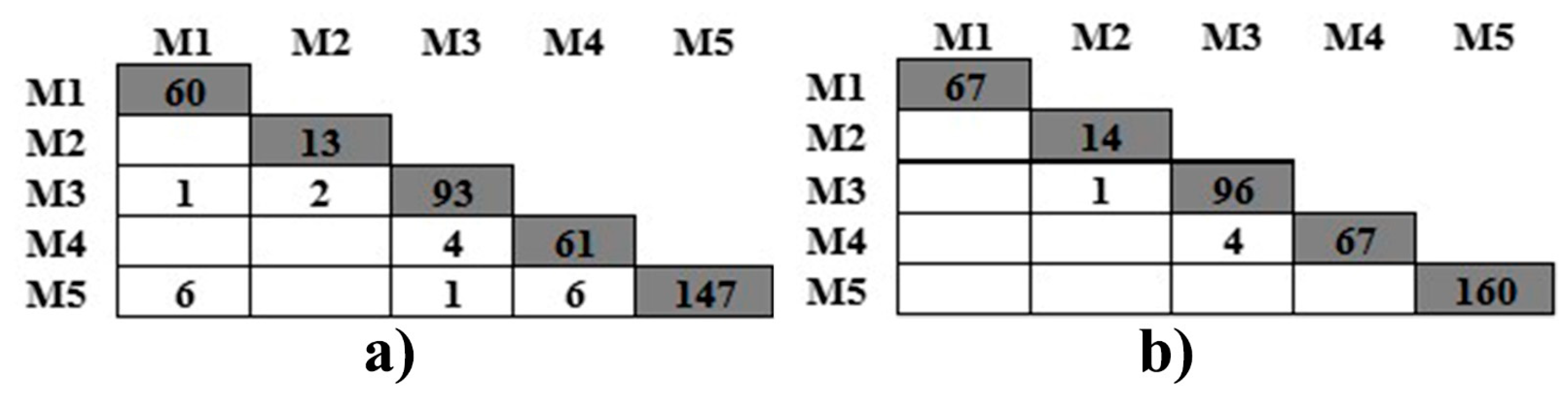
The number of effective records about methyl mercaptan concentrations at M1–M5 was 8130, 8324, 887, 8617, and 8478, respectively. A lack of data was due to instrument failures. The threshold for methyl mercaptan concentration, set in the alarm system, was 0.007 mg/m3 according to MEEPRC (1993) [23]. There were 67, 15, 101, 71, and 160 violation records at M1–M5, respectively. The highest concentration of methyl mercaptan was 0.618 mg/m3, which was observed at M5. It could be presumed that the industrial park was the main pollution source area from the wind direction statistical results of pollution events, and a few pollution incidents might be from out of the study region, as shown in Figure 2, which meant sources in residential areas outside the industrial park had few contributions to methyl mercaptan pollution. Most pollution episodes at M1 occurred under wind from east-southeast (ESE), south-southwest (SSW), and west-southwest (WSW) directions. As can be seen from 
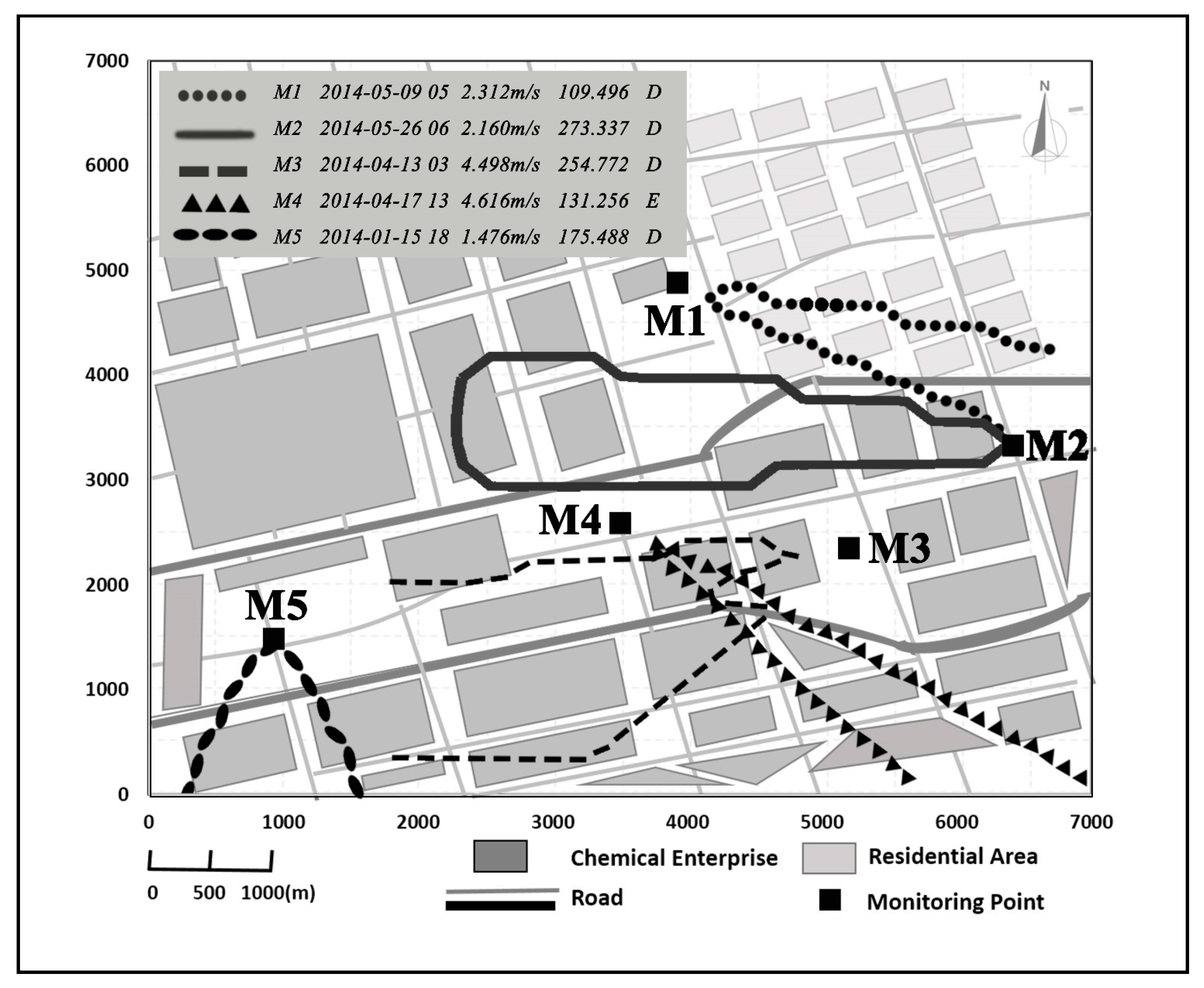
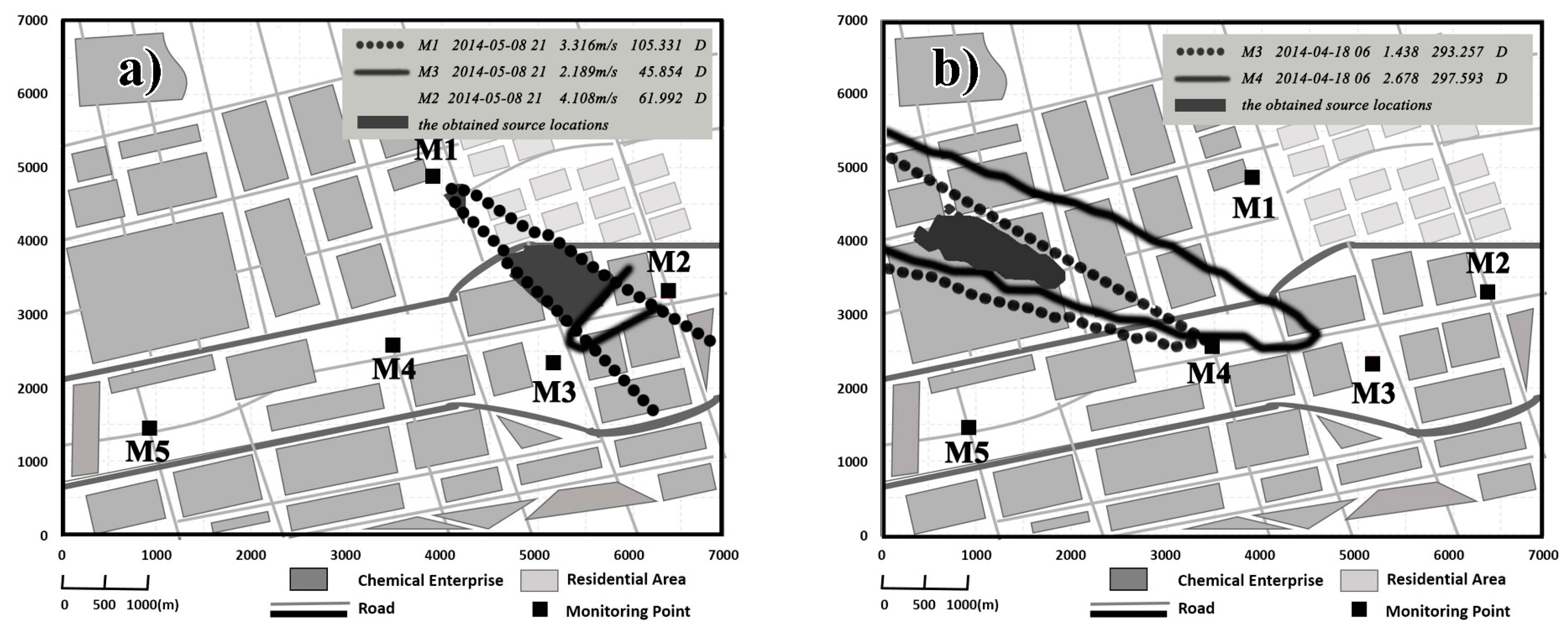
Figure 2, the exceedances at M2 were mainly related to the westward wind. The main wind directions were WSW, east (E), ESE, and west-northwest (WNW) for exceedances at M3; northwest (NW), ESE, and southeast (SE) for exceedances at M4; and south-southeast (SSE) and south (S) for exceedances at M5. It seems that the main sources for pollution episodes at M5 are independent of the episodes at other sites. Similarly, the sources with wind direction of WSW at M1, and with wind direction of E at M3, are also independent of the sources at other sites. However, there might be some links among some pollution episodes. For example, a certain consistency might be discovered between the sources responsible for the episodes at M3 with wind direction of WNW, and the sources related to the episodes at M4 with wind direction of ESE due to their relative positions. These are preliminary diagnoses only, based on the relationships between site distributions and wind directions. Further evaluation on the possibility of those pollution episodes from the same sources would be carried out via source area analysis, which addresses the impacts of wind speed and atmospheric stability in addition to that of wind direction.
Besides, the differences in wind speed and other wind direction characteristics could not be ignored. More than 80% of meteorological conditions were with wind speed of 1–4 m/s and with the atmospheric stability of D–F in this study, as shown in Figure 3. The real-time wind speed difference between the contaminated station and other stations was between 0.001 m/s and 6.414 m/s, and the real-time wind direction difference was in the range of 0°–178.457° at the same time. As can be seen in Table 2, the highest wind speed difference appeared between M1 and M4, with a maximum of 2.421 m/s. The wind speed values at M1 were generally lower than values at other stations. By contrast, the wind speed values at M4 were higher than those at other stations. The largest wind direction difference occurred in M3 and M5, with a maximum of 40.364°.
It can be seen that the local wind flow in this region is very complicated. As demonstrated in the literature, the complexity of wind field in industrial parks results from the complex underlying surface factors, such as terrain, plant canopy, various buildings, and equipment [21,24,
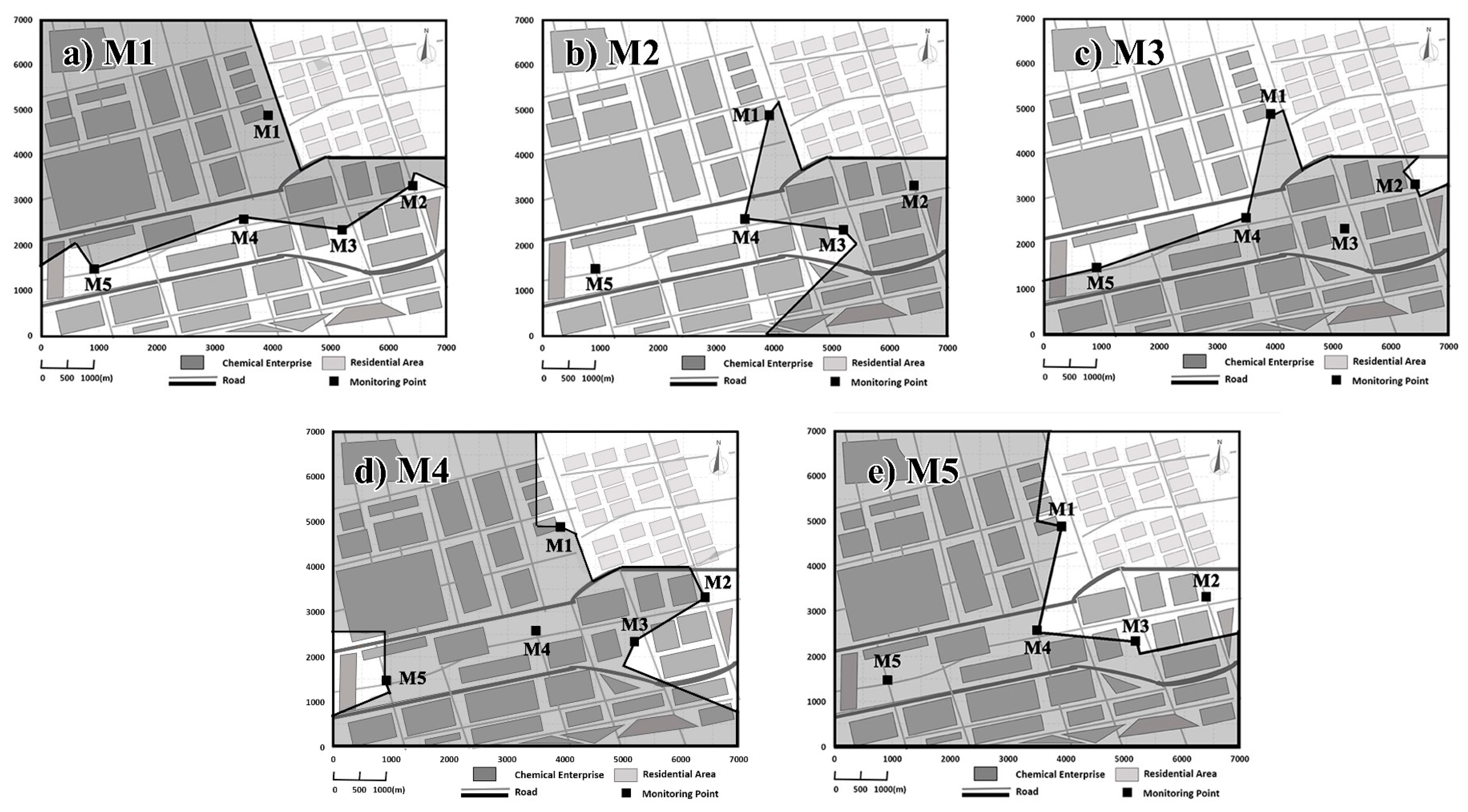
25]. With complex processes at microscales and limited information, the high-precision models, like CFD, are inapplicable. In this study, actual meteorological data were directly used in the calculation for source identification. Although they were probably not the true wind value in local environment, they were more suitable to describe the characteristics of the regional flows than the observations from the meteorological station which is located several kilometers to the east of M2. Representative regions were defined for each site to avoid misjudgment of the remote-distant pollution sources considering the strong wind differences.

3. Method

3.1. Analysis Process for Source Identification

We outlined the process of statistical source area analysis method to obtain the spatial frequency distribution of the key potential source locations (summarized in Figure 4). There were two important pre-processing steps: screening out violation records and defining the representative regions for each station, starting from the long-term meteorological and concentration measurements, which were then input into the procedure, and independent pollution episodes, as well as calculation scenarios, were identified. Next, source area analysis method was employed to back-calculate source area results for each independent pollution episode. Finally, the frequencies of grid cells as potential source locations were summarized to obtain the spatial frequency distributions of the key potential source locations for each station and the study region. The detailed procedure was organized as follows.

3.1.1. Representative Regions for Each Monitoring Station

A representative region was defined for each site to avoid misjudgment of the remote distant pollution sources, considering the strongly inhomogeneous wind distribution. Wind monitoring site A was taken to represent the whole computation area with a wind direction, if no other sites exist in its upwind or if the wind direction was consistent or adjacent with that at A; otherwise, the representative region was set to be bordered by the upwind sites. The latter case was much more common in this case study. The representative regions were defined according to the actual wind directions at each pollution incident. The smallest representative regions of each station were shown in Figure 5. The residential area on the east of M1 and the north of M2 was excluded from the representative regions, considering there were no emission sources there.

3.1.2. Recognition of Independent Pollution Episodes

A pollution event would be recorded by the monitoring system if the concentration of an ambient pollutant exceeds the alarm limit. The time interval of concentration records was set to one hour, and pollution incidents lasting over an hour were considered as two or more pollution events to make sure that the frequency statistics of the source area could represent the frequency of ambient pollution.
The pollution episodes that resulted from adverse meteorological conditions were excluded first. This was done as per the concentration change of SO2 and methyl mercaptan. SO2 emission sources were mainly fossil fuel combustion sources, which were irrelevant to emission sources of methyl mercaptan. Bad weather would be considered as the cause of the elevated methyl mercaptan concentrations if their concentration variations were in good consistency. Time series analysis by means of the statistical Pearson correlation was employed to evaluate their consistency in the concentration variations [26]. The time period before and after the pollution incident was selected, and it was needed to ensure that the pollution event happened in the middle of the selected time period as much as possible. Examples on consistency judgment were shown in Figure 6.
Independent pollution episodes were identified, and were then divided into different calculation scenarios for source area analysis through semi-empirical judgments and mistake trials. Primary judgments were based on the site distribution and wind directions at the concerned sites. Each independent pollution episode was an ambient pollution episode related to only one source which would be simulated, as required, by source area analysis method. If concentration elevations occurred at only one site, they would be directly treated as independent episodes. When multiple sites detected with a synchronous increase in concentration, a primary judgment as to whether they have the possibility to share the same sources was operated, according to the consistency between their relative locations and their wind directions. Further judgments, by means of source area analysis method, were required to ensure they were caused by the same source. Source area analysis method would provide an empty solution set if the pollutions at two or more sites were caused from various sources. Hence, if there were more than one site with excessive concentrations, site distribution and wind directions at the concerned sites would be reviewed to make a primary judgment on whether they were independent pollution episodes. If they were in good consistency, the pollution episodes at different sites would be considered as one independent episode. If the output of source area analysis method was empty, the pollution episodes at these sites did not share the source, and their source areas must be recalculated individually for each site.
Calculation scenarios of source area analysis were classified by the site number with concentration elevations and the site number involved in one run of source area analysis method. In most source identification scenarios, at a certain hour, only one site with violation records was used in the calculation, although one or two sites detected violation records. In other cases, multiple sites at a certain hour were involved in the calculation. Sometimes all violation sites were used for calculation. Sometimes non-violation sites were also added into the calculation to avoid misjudgment of potential source locations when they were just located in the upwind of the concerned violation sites. If emission from the grid source in the potential source locations would cause the concentration increase of auxiliary monitors in certain conditions, the grid would be removed from the potential source area.

3.1.3. Analysis and Statistics for Source Area Results

Source area analysis method was utilized to estimate source area distribution for each pollution episode. The industrial park was meshed, and the center of each grid cell was viewed as a virtual point source. The grid cells out of the representative regions for a monitoring site were excluded in the calculation. The rationality that these virtual sources might be the contributors to the concentration elevations was elevated one by one. A multiple run of source area analysis method provided a collection of potential sources. After obtaining source area results of all pollution events, the frequencies of each grid cell as a potential source were summarized.

3.2. Calculation Method

3.2.1. Source Area Analysis Method

Source area analysis method, proposed by Huang et al., is developed for estimating the distribution of possible source locations where there is not enough input data for explicit back-calculation of source data [7]. This method is especially suitable for source identification from lots of similar emission sources with only limited observations on the spatial concentration distribution and little prior information on sources.
Some assumptions are established as follows: (1) There is only a single emission source in each pollution incident. (2) All emission sources are point sources. (3) Concentration changes in the monitoring stations with time are mainly related to the changes of source strengths and meteorological conditions.
The basic input data required by source area analysis method are the concentration and wind measurements at monitoring sites. Optimal input data includes source parameters like source location, source height, start and end time of emission, emission rate etc. Default ranges of values would be used if no data are provided. In this case study, the whole production area of the industrial park was taken as the solution domain. The study domain was divided into a 13 × 13 grid. The grid size was 500 m × 500 m. A virtual point source was set at each grid center with 269 grid points. Feasible combinations of source parameters, mentioned above, were then searched in the given range of parameters values. According to the investigation, the source height in this case study ranged from 15–85 m. The source emission was assumed to last for one hour considering that the pollution episodes were in hourly records, and the start of source emission ranged from one minute to three hours before the time of a pollution episode. The range of emission rate was from 0 to 37 kg/h. The upper limit of the start time was set by trial runs of dispersion models, to ensure that the emission from the far end of the park was considered under low wind. The upper limit of source emission rate was also set by trial calculations. The emission of 37 kg/h, from a source at the far end of the park, could make the observed concentration rise to a hundred times of the concentration limit of methyl mercaptan under the good conditions. The prediction error of the feasible solution is defined as follows [7]:
e r r = 10 | l o g C s C m | ,
where C s and C m are the simulated and observed concentrations, respectively. In the back-calculation process, the simulated concentrations and the observed concentrations are matched at the same moment of the observation data [7]. Besides, the prediction error of the obtained source area by source area analysis method is also below this limit. Actually, the prediction error in Equation (1) is a composite indicator of the observation error, and it is hard to separate each source term error and others. When a set of variable values was within a small prediction error, they would be accepted as a feasible solution. Once a feasible solution was found for a source location, the source location would be accepted into the output source area. Err = 4 was adopted as the prediction error limit in this study [7]. It can be realized that the uncertainty of errors and parameters have been fully considered in this approach. It demonstrates all possible source regions are involved in results in all hypothetical situations. The synthetic and conservative optimization results, rather than optimal results, are obtained.

3.2.2. Gaussian Puff Model

Gaussian puff model was employed to the diffusion process simulation after the release of methyl mercaptan in source area analysis method. The simulated concentration is given by
c i ( x , y , z , t ) = Q i ( 2 π ) 3 2 σ x σ y σ z e x p [ ( x x i ) 2 2 σ x 2 ] e x p [ ( y y i ) 2 2 σ y 2 ] { e x p [ ( z z i ) 2 2 σ z 2 ] + e x p [ ( z + H i ) 2 2 σ z 2 ] ) ,
where c i ( x , y , z , t ) is the contaminant concentration at the site ( x , y , z ) downwind from puff i at ( x i , y i , H i ) , Q i is the total emission mass of the pollutant in a puff, t is the release time, H i os the effective emission height, and ( σ x , σ y , σ z ) are the dispersion coefficients in the horizontal, crosswind, and vertical directions. These coefficients were calculated as the functions of the dispersion distance based on [27]. Besides, the calculation process of power function wind speed profile mode and vertical wind speed correction were provided in the guideline [27].
The concentration contribution of all puffs at ( x , y , z ) in the downwind at time t was calculated according to
c ( x , y , z , t ) = i = 1 n c i ( x , y , z , t ) ,
where n means the number of the puffs.
The actual observations of wind speed and wind direction were employed in the calculation process. Atmospheric stability classifications were determined by means of temperature gradient—wind speed method (ΔT/U). Inside, the detailed standard was shown in the Table “Standard of stability classification using temperature difference—wind speed method” [28]. The temperature gradients were calculated by sounding data, which were provided by University of Wyoming for the Shanghai radio-sounding stations (http://weather.uwyo.edu/upperair/sounding.html, Site No. 58362) [29]. Besides, the data were obtained for two times per day (08:00 and 20:00 CCT). Thus, the stabilities at 0800 were also employed for the calculation of pollution events at 02:00 to 14:00, and those at 2000 were employed for the calculation at 14:00 to 02:00.

4. Result

4.1. Statistical Results of Independent Pollution Episodes

A total of 414 violation records were indexed by the alarm system in 2014. Some of them appeared simultaneously. Figure 7a presented the frequencies of violation records at different sites. The diagonal values in the lower triangular matrix displayed the frequencies of violation records at a single site, and the others were the frequencies of simultaneous violation records at two sites. It could be seen from Figure 7a that 414 violation records, only, shared 394 h. Forty violations occurred simultaneously at two sites and covered 20 h. Only one violation record appeared at M1 and M3 simultaneously, and the same with the frequency at M3 and M5; six violation records simultaneously appeared at M1 and M5, which was the same as at M4 and M5; the violation records at M2 shared four hours with those at M3.
Thirty-five independent pollution episodes were determined for these forty violation records. Only five independent pollution episodes involving two sites were found in the statistic frequencies of independent pollution episodes shown in Figure 7b. It also indicated that M2 and M3 were involved in an independent episode once and M3 and M4 were involved in an independent episode four times. According to the method for determining independent pollution episodes in Section 3.1.2, other violation records were treated as independent pollution episodes of a single site. No record involving three or more violation monitoring sites was found in this case.
In sum, 404 violation records were considered as independent pollution episodes of a single site (diagonal values in Figure 7b) and another 10 were considered as five independent pollution episodes of two sites (off-diagonal values in Figure 7b). In addition, there was only one case where the concentration data of a nearby site was involved in source area analysis to kick out misjudged source locations, since it was below the alarm limit.
Finally, independent pollution episodes were classified into three types of typical scenarios for source identification calculation: (i) scenarios where only one violation site was involved; (ii) scenarios where two violation sites were used for identifying source locations; (iii) scenarios where multiple sites were involved for identifying source locations, but there was only one site with abnormally elevated concentrations.

4.2. Source Area Results of Typical Scenarios

4.2.1. Scenarios with a Single Violation Site

Most scenarios in this study were those where the data of only one single violation site were used for identifying source locations. Inside, most of them were the situations where only one single site had abnormally elevated concentrations. There were a few instances of two violation sites occurring at the same time. The typical source area of pollution incidents at each site, under their own dominant winds as examples, are provided in Figure 8.
The presented results in Figure 8 happened at various times at M1–M5. Most pollution episodes at M1 occurred with wind direction of ESE, SSW, and WSW (Figure 2), including a small area in the northeast of the industrial park. The case of M1 happened at 05:00 on 9 May 2014, with a wind direction of 109.5°. Meanwhile, the wind direction of M2 and M3, which are located in the upwind region of M1, were 79.0° and 198.8°, respectively. As a result, their wind directions were inconsistent with those of M1. The calculation domain range of M1 was limited to the M2 and M3 cutoffs, avoiding the misjudgment of source locations.
Source areas of most pollution episodes at M3 and M4 appeared in the WSW regions of M3 and the southeast regions of M4. There were no other sites in their upwind directions, different with the example at M1. Thus, the whole regions upwind of their high-frequency wind directions were adopted into the search domain. The obtained source locations are shown in Figure 8. Obviously, much larger source area was searched compared with the results of M1. In the pollution episode at 03:00 on 13 April 2014, the wind direction at M3 was 254.772° (WSW), one of its dominant wind directions, while the wind direction at M5, which located in the upwind region of M3, was 307° (NW). With the inconsistent wind directions, the source area at M3 with wind direction of WSW ended at M5.
As illustrated in Figure 8, the southern regions of M5 represents its typical source area. This station was located in the southern boundary of this industrial park with small search range, which contained a much smaller number of pollutant sources than the other sites. As a result, the range of the obtained feasible solutions could be concentrated in a small region in the south, due to the smaller search range. Cases like this were the most advantageous situations using a single site’s data for source identification. Unfortunately, it is not realistic to expect all episodes under idealized situation. For example, interference sources around the real source could not be ruled out in calculation processes of M2/M3/M4 because of limited information and larger search ranges, although only one emission source was responsible for the elevated concentration.
It is also presented in Figure 8 that wind direction played an important role for source area results. Also, wind speed and atmospheric stability also had significant impacts on source area results. The results under different meteorological conditions at one site are summarized in Figure 9. To make it clear, two cases in different wind speeds were selected as examples. Actually, source locations were mainly related to meteorological conditions rather than pollutant concentration in single-site scenarios. Therefore, the characteristics of source area results were the same no matter which site was selected. The results in terms of low-wind-speed and high-wind-speed are shown in Figure 9a,b. Here, the high-wind-speed condition is greater than 1.5 m/s. Figure 9 indicates that the lateral width of obtained source areas would be smaller with the increment of atmospheric stability independent of the wind speed, and it also indicates that the lateral width of source areas obtained in low-wind-speed was relatively larger compared with that in higher-wind-speed under the same atmospheric stability. The different transport and diffusion abilities of pollutant in different meteorological conditions were explained by Arya S P [30]. We can conclude that it is more favorable for source identification under windy and stable weather conditions if there is only a single violation source.

4.2.2. Scenarios with Multiple Sites

Source area results at M1 from the pollution episode at 21:00 on 8 May 2014 are shown in Figure 10a. Concentration measurements at M1 had been over the alarm limit for twenty hours, while concentrations of other sites were below the limit. During the period, the dominant wind direction of M1 was 105.331° (SSE). Meanwhile, those of M2 and M3 were 62° (east-northeast, ENE) and 45° (northeast, NE), respectively. Theoretically, both M2 and M3 could be used for source identification as assistant monitoring sites. In fact, only M3 could be used as an assistant monitoring site because if M2 recorded a pollution episode, the determined source locations were no overlap with those of M1. In such a strategy, the determined source area of M1, in this case, was found in the distance of 2.4–3.2 km above its upwind direction, as shown in Figure 10a.
The results for the scenario at 06:00 on 18 April 2014 are presented in Figure 10b, where M3 and M4 were with abnormally elevated concentrations simultaneously. There were no abnormal concentration changes of methyl mercaptan at other sites and no consistent changes of SO2 at these two sites at that time. M3 was with wind direction of 293° (WNW) and M4 was with wind direction of 296° (WNW). They had consistent wind directions and there was a large overlap in their upper wind directions. Thus, they were analyzed as an independent pollution episode with a homologous source at first, and the obtained source area was shown in the shaded region. The common source area lay in the upper wind direction of M4 with the distance of 0.8–2 km, based on the above assumption. Besides, the source area results of M3 and M4 calculated as two independent pollution episodes were also displayed in Figure 10b. It can be seen two source area results are overlapped partially, indicating that they might be caused by the same source. The overlapping region between the presented source areas of M3 and M4 are larger than the shaded source area. The reason is that solutions of other parameters during the overlapping region, such as source height and emission time, might be different when two source location solutions at M3 and M4 are searched. In contrast, all source parameters are the same, and errors are below the error limit simultaneously during the calculation process of the shaded source area.

4.3. Spatial Frequency Distribution of Source Areas

The total frequency results of obtained source locations from all pollution records are shown in Figure 11. The statistical results for all scenarios where only a single site was used for source identification are displayed in Figure 11a–e. Figure 11f shows the frequency results of all obtained source locations, including scenarios where a single site and multiple sites were used for source identification. It could be concluded that (1) the high-frequency source area at M1 is located in its eastern region; (2) the high-frequency source area at M2 is not obvious, due to its few violation records; (3) the high-frequency source area at M3 is the regions of east and west-southwest directions; (4) the high-frequency source area at M4 is in the northwest direction; (5) the regions in the south of M5 are the high-frequency source areas. The high-frequency source locations in the study region distributes on the southern regions of M5, and slightly eastern regions of the plot after superimposing all the frequency results (Figure 11f). Comparing Figure 11c,e with Figure 11f, it is easy to conclude that the key potential source locations are mainly related to the pollution episodes of M5, and are slightly affected by the pollution episodes of M3. The contribution from the latter is much smaller than the former. According to the on-site investigations from environmental protection departments, there is a set of oily wastewater treatment equipment in the high-frequency source regions, which does, indeed, have the possibility of methyl mercaptan emissions.
There is another high-frequency region appeared between M3 and M4. The frequency of source locations in this region is lower than that in the southern region of M5 (Figure 11f). The overlapping source locations for M3 and M4 revealed the possibility of the high-frequency source region. Emissions from this region might improve the concentration measurements at M4 with wind direction of SE and, meanwhile, concentrations at M3 have increased with the wind direction of WNW. Therefore, there is a small probability that a constant source emission from this region would elevate the concentrations at M3 and M4 simultaneously, due to their positions relative to the high-frequency source locations. There was no such case in 2014. There is an important odor pollution area in this high-frequency region, but it is not certain whether it is indeed a source of methyl mercaptan pollution according to the on-site investigations. In addition, the region in the northwest of M4 is also a high-frequency area in Figure 11f. It is mainly related to the pollution events of M4, M1, and M5. Based on their relative orientations and distances, the possibility is very small that three monitors had the elevated concentration, at the same time, when the emission was from this region. According to the investigations, there is a coating company in this area, which indeed has the possibility of methyl mercaptan emissions.
Figure 11a presents two regions around M1 with more than 14 frequencies traced by back-calculation of pollution episodes. The frequency of these two regions accounted for 53.70% of the total frequency of independent episodes at M1 from Figure 2 and Figure 7b. Similarly, the areas located in two high-frequency wind directions of M3 in Figure 11c have more frequencies to be traced, making up a 55.21% share of the total frequencies of the independent episodes at M3. Figure 11d illustrates that the northwest and southeast regions of M4 belong to high-frequency source areas. In the pictures above, it is clear that the high-frequency region around M2 is not obvious, due to having the fewest violation records and its unstable wind. M5 had the most violation records, and its pollution wind directions were concentrated in the southeast and south directions, as shown in Figure 2. Therefore, the obtained source areas were concentrated on their upwind regions, and the cumulative frequency in these wind directions accounted for 59.38% of the total frequencies of M5. As displayed in Figure 11e, the frequency around M5 is gradually reduced from the intermediate maximum value to both sides. Two reasons can explain the regular frequency distribution: one is the overlay of obtained diverse resolutions under different atmospheric stabilities with the same dominant wind direction; the other is the overlay with the adjacent wind directions. Concentration observations at M5 would be easily elevated under both of the two wind directions.

5. Conclusions and Discussion

This work presents source identification cases based on long-term abnormal concentration measurements of methyl mercaptan in an industrial park with five fixed monitoring sites. There is a little possibility that an excessive emission caused the abnormal concentration changes of multiple sites at the same time or over several hours, due to the large area of the park and the sparse distribution of monitoring sites. In the case of all violation records, most are pollution episodes where abnormal concentrations were only observed at a single site. A few were episodes where two sites had simultaneous violations, and there were no episodes where three sites reached the alarm limit simultaneously. Source identification process mainly relies on ambient observations, including meteorological and concentration data. The huge number of long-term observations in 2014 were addressed for source identification analysis in the current study. Fortunately, they inspired us to develop a statistical method for source identification.
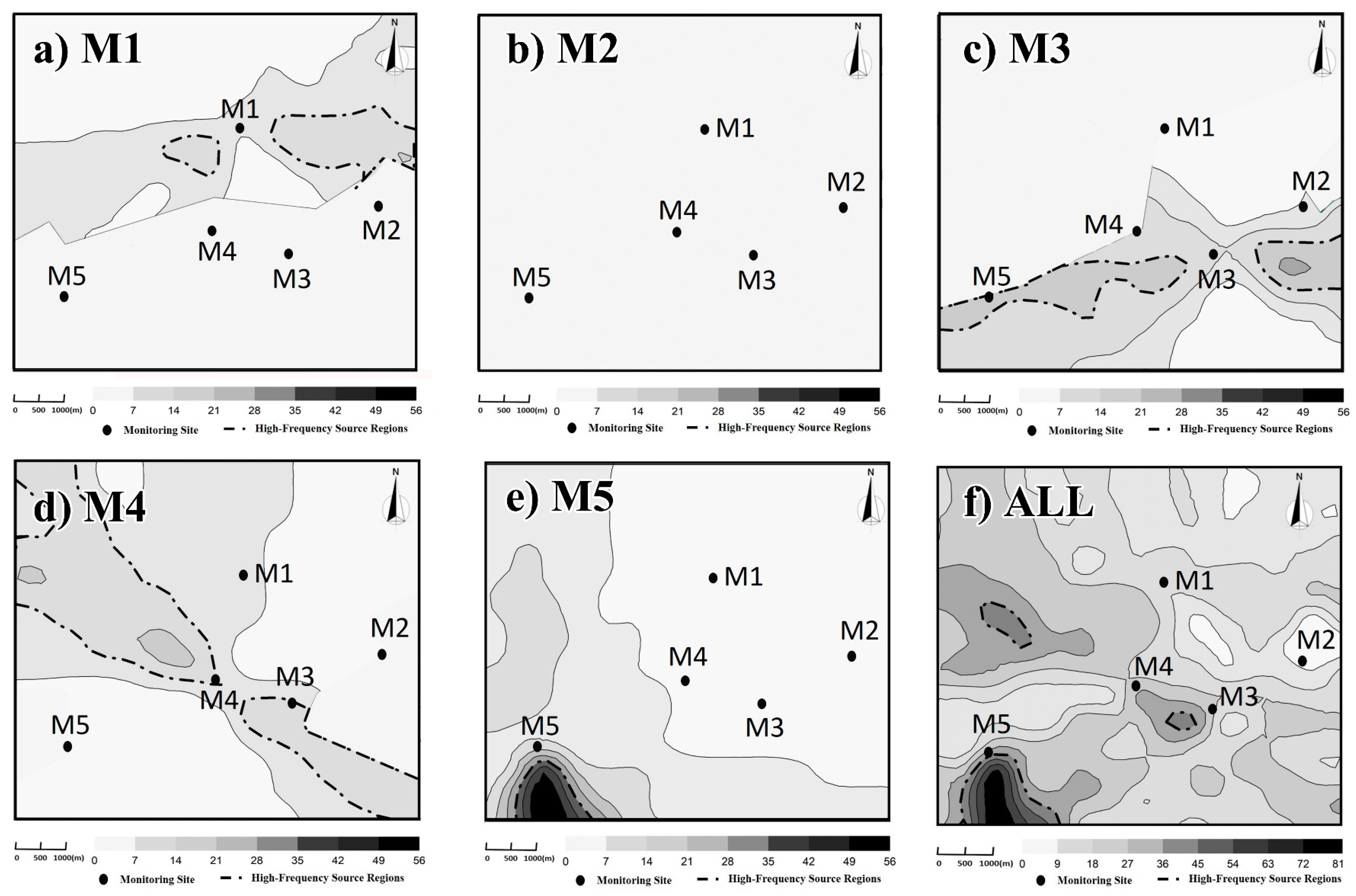
A statistical approach for source identification by means of long-term monitoring data is provided, including the selection of representative regions, the determination of independent pollution episodes and calculation scenarios, the back-calculation of the source area, and the statistical analysis of the obtained results. In the end, the spatial frequency distributions of the key suspected source locations are obtained. From the perspective of the high-frequency source regions, there is little possibility that pollutant emissions located in these regions can bring about multiple sites’ concentration changes simultaneously. This is consistent with the characteristics of a monitoring network for pollution events which are reflected by the observation data of each pollution incident. Under such a monitoring network, the source area obtained by one running calculation of a single site did not have a strong guide. By contrast, the spatial-temporal frequency statistical overlay analysis of the obtained source locations provides more direct information for pollution control.
A prerequisite for getting more accurate source information through spatial-temporal overlay analysis is, possibly, that potential common source areas are discovered from independent episodes at different monitors and different times. If some sources release pollutant regularly, pollution incidents at different sites and times will point at the actual emission sources. High-frequency source areas, in this paper, mainly appeared in two situations. Most of them appeared in the regions with a high-frequency wind direction of pollution incidents at every single site. If the high-frequency wind directions of pollution incidents at a certain site are adjacent, just like the ones of M5, its contribution to the high-frequency source region is more obvious after the overlay. In another situation, the high-frequency source area appeared due to the overlays of potential source areas from pollution incidents of multiple sites. As per the sparse monitoring network, few suspected cases appeared where a source emission caused the increased concentrations of multiples sites. In this study, the overlapping source area from M3 and M4, as well as the overlapping source area from M3, M1, and M5, belongs to this kind of situation. Emissions from the regions might lead to the concentration increase of one or several sites, at different times and under different conditions.
Admittedly, the uncertainties in source area results mainly come from the limited basic information of the studied case. There are many uncertainties in this methodology, due to limited monitoring site information. Also, absent prior information on the source adds difficulties to accurate source identification. Source area analysis method is expected to be a good approach to find meaning from limited information and uncertain factors. The uncertainties of source parameters had been considered partially, and all feasible solutions are obtained through the optimal solution for the uncertain source parameters (described at length in Section 3.2.1).
In addition to above factors, the representative error of meteorological data also has a significant impact on the obtained source area results. Further study will be intended to develop the simulation technologies for the local subgrid complex flow field, due to large spatial uniformity and complexities of the meteorological flow in this study area. The simulation technique, in this paper, takes meteorological data of every single site for calculation, rather than using the refined technique for complex flow field. The representative region of each site is determined according to real-time meteorological conditions, to avoid the misjudgment of feasible solutions caused by the uncertainties of the remote flow field. Such simplification might inevitably result in a lower statistical frequency of source locations in the far regions in some cases. There is still a certain error within the representative regions. The meteorological observation analysis in Table 2 indicates that the real-time wind direction difference among five stations might be between 0°–178.457°, and the real-time wind speed difference might be between 0.001–6.414 m/s. It is very difficult to estimate the representation errors accurately, due to the unavailable real wind values. Thus inverse distance weighted (IDW , power = 2, [25]) is selected to calculate the real wind reference value, then compared with the uniform meteorological measurements within the representative regions, to assess the spatial nonuniformity level. A, B, and C, surrounded by M1–M3, are defined as test points for analysis, as plotted in Figure 1. The distances to M1 from A, B, and C are 800, 1600, 2400 m, respectively. This region is the most appropriate area for interpolation analysis throughout the total computational domain because there are three monitoring stations surrounded. There are twelve pollution incidents with wind direction of ESE where three test points are located in its upwind direction of M1. In these records, the average pollution wind speed of M1 is 2.098 m/s, and the average pollution wind direction is 108°. The interpolated average wind speeds of A, B, and C are 2.154, 2.360, and 2.595 m/s, respectively, and the interpolated average wind directions are 106°, 101°, and 100°, respectively. It could be concluded that the closer it is to M1, the slighter the error in wind speed is. This also applies to wind direction. From the view of wind direction, a certain deviation existed between the interpolated wind directions of A, B, C, and the observed wind direction of M1. However, the error level is acceptable because the interpolated wind directions are near ESE. In general, the representative error of meteorological data is still a problem worth further research. Besides, the influence of buildings and other obstacles in canopy layer on vertical wind shear, wind measurements, and atmospheric turbulence also deserve more exploration. Refined simulation techniques are required to be developed for such local complex regions in future research, especially in industrial parks with plenty of production equipment and dense underlying surface, which are also the technical basis for the refined source identification results. Attempts to couple the urban canopy model in the weather research and forecasting model (WRF) with CFD, and the explicit explorations of atmospheric stability levels, might be considered for further study in meteorological perspectives.

Author Contributions

Y.L. calculated the data and wrote this paper; Q.Y. reviewed the general idea in this paper; Z.H. provided constructive discussions; W.M. and Y.Z. made some suggestions for this the paper.

Funding

This study was supported by the project of Science and Technology Commission of Shanghai Municipality (No. 15DZ1205303).

Conflicts of Interest

The authors declare no conflict of interest.

Abbreviations

The following abbreviations were used in this manuscript:
ESEEast-southeast
SSWSouth-southwest
WSWWest-southwest
EEast
WNWWest-northwest
NWNorthwest
SESoutheast
SSESouth-southeast
SSouth
ENEEast-northeast
NENortheast

References

  1. Cantelli, A.; D’Orta, F.; Cattini, A.; Sebastianelli, F.; Cedola, L. Application of genetic algorithm for the simultaneous identification of atmospheric pollution sources. Atmos. Environ. 2015, 115, 36–46. [Google Scholar] [CrossRef]
  2. Thomson, L.C.; Hirst, B.; Gibson, G.; Gillespie, S.; Jonathan, P.; Skeldon, K.D.; Padgett, M.J. An improved algorithm for locating a gas source using inverse methods. Atmos. Environ. 2007, 41, 1128–1134. [Google Scholar] [CrossRef]
  3. Keats, A.; Yee, E.; Lien, F.S. Bayesian inference for source determination with applications to a complex urban environment. Atmos. Environ. 2007, 41, 465–479. [Google Scholar] [CrossRef]
  4. Sharan, M.; Singh, S.K.; Issartel, J.P. Least Square Data Assimilation for Identification of the Point Source Emissions. Pure Appl. Geophys. 2012, 169, 483–497. [Google Scholar] [CrossRef]
  5. Penenko, V.; Baklanov, A.; Tsvetova, E. Methods of sensitivity theory and inverse modeling for estimation of source parameters. Future Gener. Comput. Syst. 2002, 18, 661–671. [Google Scholar] [CrossRef]
  6. Rudd, A.C.; Robins, A.G.; Lepley, J.J.; Belcher, S.E. An Inverse Method for Determining Source Characteristics for Emergency Response Applications. Bound.-Layer Meteorol. 2012, 144, 1–20. [Google Scholar] [CrossRef]
  7. Huang, Z.; Wang, Y.; Yu, Q.; Ma, W.; Zhang, Y.; Chen, L. Source area identification with observation from limited monitor sites for air pollution episodes in industrial parks. Atmos. Environ. 2015, 122, 1–9. [Google Scholar] [CrossRef]
  8. Haupt, S.E. A demonstration of coupled receptor/dispersion modeling with a genetic algorithm. Atmos. Environ. 2005, 39, 7181–7189. [Google Scholar] [CrossRef]
  9. Haupt, S.E.; Young, G.S.; Allen, C.T. A Genetic Algorithm Method to Assimilate Sensor Data for a Toxic Contaminant Release. J. Comput. 2007, 2. [Google Scholar] [CrossRef]
  10. Yee, E. Inverse Dispersion for an Unknown Number of Sources: Model Selection and Uncertainty Analysis. ISRN Appl. Math. 2012, 2012, 1–20. [Google Scholar] [CrossRef]
  11. Zheng, X.; Chen, Z. Back-calculation of the strength and location of hazardous materials releases using the pattern search method. J. Hazard. Mater. 2010, 183, 474–481. [Google Scholar] [CrossRef] [PubMed]
  12. Singh, S.K.; Sharan, M.; Issartel, J.P. Inverse Modelling for Identification of Multiple-Point Releases from Atmospheric Concentration Measurements. Bound.-Layer Meteorol. 2013, 146, 277–295. [Google Scholar] [CrossRef]
  13. Wawrzynczak, A.; Kopka, P.; Borysiewicz, M. Sequential Monte Carlo in Bayesian Assessment of Contaminant Source Localization Based on the Sensors Concentration Measurements. In Proceedings of the International Conference on Parallel Processing and Applied Mathematics, Warsaw, Poland, 8–11 September 2013; Springer: Berlin/Heidelberg, Germany, 2013; pp. 407–417. [Google Scholar]
  14. Allen, C.; Young, G.; Haupt, S. Improving pollutant source characterization by better estimating wind direction with a genetic algorithm. Atmos. Environ. 2007, 41, 2283–2289. [Google Scholar] [CrossRef]
  15. Hosseini, B.; Stockie, J.M. Bayesian estimation of airborne fugitive emissions using a Gaussian plume model. Atmos. Environ. 2016, 141, 122–138. [Google Scholar] [CrossRef] [Green Version]
  16. Haupt, S.E.; Beyer-Lout, A.; Long, K.J.; Young, G.S. Assimilating concentration observations for transport and dispersion modeling in a meandering wind field. Atmos. Environ. 2009, 43, 1329–1338. [Google Scholar] [CrossRef]
  17. Annunzio, A.J.; Young, G.S.; Haupt, S.E. Utilizing state estimation to determine the source location for a contaminant. Atmos. Environ. 2012, 46, 580–589. [Google Scholar] [CrossRef]
  18. Khajeh Najafi, S.; Gilbert, E. Use of real-time measurements for estimating release rate. In Proceedings of the Hazards XVII. Process Safety—Fulfilling Our Responsibilities: Institution of Chemical Engineers Symposium Series, Manchester, UK, 25–27 March 2003; pp. 155–171. [Google Scholar]
  19. Chow, F.K.; Kosović, B.; Chan, S. Source Inversion for Contaminant Plume Dispersion in Urban Environments Using Building-Resolving Simulations. J. Appl. Meteorol. Climatol. 2008, 47, 1553–1572. [Google Scholar] [CrossRef] [Green Version]
  20. Kovalets, I.V.; Andronopoulos, S.; Venetsanos, A.G.; Bartzis, J.G. Identification of strength and location of stationary point source of atmospheric pollutant in urban conditions using computational fluid dynamics model. Math. Comput. Simul. 2011, 82, 244–257. [Google Scholar] [CrossRef]
  21. Ma, X.; Zhong, W.; Feng, W.; Li, G. Modelling of pollutant dispersion with atmospheric instabilities in an industrial park. Powder Technol. 2017, 314, 577–588. [Google Scholar] [CrossRef]
  22. Mei, D.; Xing, F. Numerical analysis of pollutant dispersion from the industry stacks: Effects of Schmidt number and wind velocity. In Proceedings of the International Conference on Remote Sensing, Environment and Transportation Engineering, Nanjing, China, 24–26 June 2011; pp. 5107–5110. [Google Scholar]
  23. MEEPRC (Ministry of Ecology and Environment of the People’s Republic of China). Emission Standards for Odor Pollutants (GB14554-93). 1993. Available online: http://www.mee.gov.cn/image20010518/5303.pdf (accessed on 22 October 2018).
  24. Abdul-Wahab, S.A. Evaluation of the Industrial Source Complex Short-Term Model: Dispersion over Terrain. J. Air Waste Manag. Assoc. 2012, 54, 396–408. [Google Scholar] [CrossRef]
  25. Dehghani, M.; Taghizadeh, M.M.; Hashemi, H.; Rastgoo, E. A preliminary assessment of dispersion level of SO2 in Fars industrial region, south of Iran, by GIS. J. Environ. Public Health 2013, 2013, 1–6. [Google Scholar] [CrossRef]
  26. Kruskal, W.H. Ordinal Measures of Association. J. Am. Stat. Assoc. 1958, 53, 814–861. [Google Scholar] [CrossRef]
  27. MEEPRC (Ministry of Ecology and Environment of the People’s Republic of China). Technical Methods for Making Local Emission Standards of Air Pollutants (GB/T3840-91). 1991. Available online: http://www.mee.gov.cn/image20010518/5332.pdf (accessed on 22 October 2018).
  28. Jiang, W. Air Pollution Meteorology; Nanjing University Press: Nanjing, China, 2003; pp. 124–125. [Google Scholar]
  29. Petty, G.W. A First Course in Atmospheric Thermodynamics; Sundog Pub.: Madison, WI, USA, 2008; p. 337. [Google Scholar]
  30. Arya, S.P. Air Pollution Meteorology and Dispersion; Oxford University Press: New York, NY, USA, 1999; Volume 310. [Google Scholar]
Figure 1. Locations of monitoring stations and test points.
Atmosphere 09 00501 g001
Figure 2. Pollution wind roses at each monitoring stations.
Atmosphere 09 00501 g002
Figure 3. Comprehensive meteorological statistics in wind speed and atmospheric stability for pollution episodes.
Atmosphere 09 00501 g003
Figure 4. Flow diagram of the statistical source area analysis method.
Atmosphere 09 00501 g004
Figure 5. The smallest representative regions for M1–M5: (a) the smallest representative regions of M1; (b) the smallest representative regions of M2; (c) the smallest representative regions of M3; (d) the smallest representative regions of M4; (e) the smallest representative regions of M5.
Atmosphere 09 00501 g005
Figure 6. Examples of consistency judgment: (a) an example of the inconsistency, r = −0.3943, Sig = 0.439; (b) an example of the strong consistency, r = 0.6727, Sig = 0.047. r is the Pearson correlation coefficient in the range [–1, 1]. The sign indicates the direction of the relationship, while the magnitude indicates the strength of the relationship. Sig represents the significance test, in which 0.05 is set for statistical significance in general. A value of 0.06727 means strong correlation, −0.3943 means negative weak correlation. 0.01 < Sig < 0.05, a statistical significance; 0.001 < Sig < 0.05, highly statistically significant.
Atmosphere 09 00501 g006
Figure 7. Frequencies of violation records at monitoring sites and the corresponding frequencies of independent pollution episodes: (a) frequencies of violation records; (b) frequencies of independent pollution episodes. The diagonal values are statistical results for single-site cases and the non-diagonal values are results for two-site cases.
Atmosphere 09 00501 g007
Figure 8. Typical source area results at each monitoring site.
Atmosphere 09 00501 g008
Figure 9. Source locations under different meteorological conditions: (a) typical source area results in low-wind-speed with different atmospheric stabilities; (b) typical source area results in high-wind-speed with different atmospheric stabilities.
Atmosphere 09 00501 g009
Figure 10. Source area results of the typical scenarios with multiple sites used for source identification: (a) the results of the scenario of multiple sites for source identification, but with only one site with the abnormally elevated concentration; (b) the results of the scenario of two violation sites’ measurements used for source identification.
Atmosphere 09 00501 g010
Figure 11. The spatial frequency results of obtained source locations for various monitoring sites: (a) spatial frequency results at M1; (b) spatial frequency results at M2; (c) spatial frequency results at M3; (d) spatial frequency results at M4; (e) spatial frequency results at M5; (f) total frequency results for five monitoring sites. The numbers in the figures were the statistical frequency which represented the times that the position was counted as the suspected source locations.
Atmosphere 09 00501 g011
Table 1. Conditions of each monitoring station.
StationHeight of the SensorSurrounding Conditions
M115 mIt is placed on a three-floor building.
The sampling port is over 1 m away from the roof.
No pollution source within the range of 50 m.
M222.8 mIt is placed on a five-floor building.
The sampling port is over 1 m away from the roof.
No pollution source within the range of 50 m.
M39 mIt is placed on a low building.
The sampling port is over 1 m away from the roof.
No pollution source within the range of 50 m.
M412.5 mIt is located on a three-floor building.
The sampling port is over 1 away from the roof.
No pollution source within the range of 50 m.
M56 mA building dedicated to monitoring, which is supported by four pillars with a height of 2.5 m and a device room about 2 m in height is built above.
The sampling point is 1.5 m away from the roof.
No pollution source within the range of 50 m.
Table 2. Real-time wind speed and wind direction error for pollution episodes at each station.
Contaminated StationFrequency of Violation RecordsWind Speed Difference 1 (m/s)Wind Direction Difference 2 (°)
M1M2M3M4M5M1M2M3M4M5
M167-1.2680.6202.5750.557-−5.995−30.234−6.47316.558
M215−0.929-0.4961.790−0.522−2.409-−10.787−7.1928.468
M3101−0.7310.811-2.1230.24527.00726.999-23.20740.364
M471−2.421-0.600−1.967-−1.9249.5738.783−11.793-8.360
M5160−0.3280.6560.1781.537-6.307−9.959−37.645−8.516-
1 Wind speed difference is the average value of wind speed differences at each pollution episode. 2 Wind direction difference is the average value of wind direction differences at each pollution episode. ”-“ means that there was no difference in wind speed or wind direction.

