Abstract
Consistent streamflow forecasts play a fundamental part in flood risk mitigation. Population increase and water cycle intensification are extending not only globally but also among Pakistan’s water resources. The frequency of floods has increased in the last few decades in the country, which emphasizes the importance of efficient practices needed to adopt for various aspects of water resource management such as reservoir scheduling, water sustainability, and water supply. The purpose of this study is to develop a novel hybrid model for streamflow forecasting and validate its efficiency at the upper Indus basin (UIB), Pakistan. Maximum streamflow in the River Indus from its upper mountain basin results from melting snow or glaciers and climatic unevenness of both precipitation and temperature inputs, which will, therefore, affect rural livelihoods at both a local and a regional scale through effects on runoff in the Upper Indus basin (UIB). This indicates that basins receive the bulk of snowfall input to sustain the glacier system. The present study will help find the runoff from high altitude catchments and estimated flood occurrence for the proposed and constructed hydropower projects of the Upper Indus basin (UIB). Due to climate variability, the upper Indus basin (UIB) was further divided into three zone named as sub-zones, zone one (z1), zone two (z2), and zone three (z3). The hybrid models are designed by incorporating artificial intelligence (AI) models, which includes Feedforward backpropagation (FFBP) and Radial basis function (RBF) with decomposition methods. This includes a discrete wavelet transform (DWT) and ensemble empirical mode decomposition (EEMD). On the basis of the autocorrelation function and the cross-correlation function of streamflow, precipitation and temperature inputs are selected for all developed models. Data have been analyzed by comparing the simulation outputs of the models with a correlation coefficient (R), root mean square errors (RMSE), Nash-Sutcliffe Efficiency (NSE), mean absolute percentage error (MAPE), and mean absolute errors (MAE). The proposed hybrid models have been applied to monthly streamflow observations from three hydrological stations and 17 meteorological stations in the UIB. The results show that the prediction accuracy of the decomposition-based models is usually better than those of AI-based models. Among the DWT and EEMD based hybrid model, EEMD has performed significantly well when compared to all other hybrid and individual AI models. The peak value analysis is also performed to confirm the results’ precision rate during the flood season (May-October). The detailed comparative analysis showed that the RBFNN integrated with EEMD has better forecasting capabilities as compared to other developed models and EEMD-RBF can capture the nonlinear characteristics of the streamflow time series during the flood season with more precision.
1. Introduction
The raising population is enhancing the demand for freshwater, which results in the need for optimal water resource management [1,2]. According to Penman (1961) [3], hydrology is the science that tries to respond to the query ‘what happens to the rain’? One of the main features of this query and its response lies in the conversion of rainfall into the streamflow [4]. The rainfall and streamflow bond rests multifaceted because of spatial and temporal unevenness of watersheds, precipitation, evaporation, runoff yield and confluence, topography, and human activities. Streamflow forecasting states with the systematic evaluation of upcoming streamflow based on historical hydro-meteorological data [5,6,7] and precise streamflow forecasting assists pre-arranged preparation and managing water resources. They also caution and mitigate the natural disaster such as droughts and floods. Therefore, a proficient method to help understand the nature of such a phenomenon is necessary [8,9,10].
Over the past few decades, many researchers have proposed numerous forecasting methods to address the scarcity of the runoff data [11,12,13]. Generally, they are divided into two major categories: process-driven and data-driven methods [14,15,16]. Process-driven models like conceptual rainfall-runoff try to explain the underlying physical processes of the watershed system [17]. Data-driven models often used to make short-term predictions using simple mathematical methods and intelligent algorithms via the statistical characteristics that avoid analyzing the physical processes and instead build a “black-box” to forecast the future streamflow [18]. Data-driven methods have gained popularity in the recent past for streamflow forecasting due to obtaining the gauging data, increasing computational command, the improvement in progressive modeling theory and software, and holding off clarifying the multifarious core physical processes of the watershed system [19,20,21,22].
Most commonly used time series models are Autoregressive (AR), AR moving average (ARMA), and AR integrated moving average (ARIMA) [23]. Non-linearity is the characteristic of streamflow time series, particularly under climate and land use changes that makes AR, ARMA, ARIMA, and other linear regression models inappropriate for streamflow forecasting [24,25,26,27,28,29,30].
In hydrologic modeling, on the other hand, artificial neural networks (ANNs) introduction in the 1990s can be considered as a benchmark [31,32]. The ANNs have seemed as influential black-box models among data-driven models and acknowledged an excessive responsiveness throughout the last 20 years [33,34]. With little available data, ANN models can deliver an approach to disclose the properties of hydrological developments, which will support us to better understand the effect of environmental variations on the hydrological processes in permafrost areas [35,36]. Many scholars have used ANN models to simulate and predict runoff fluctuations because artificial intelligence models, e.g., artificial neural network (ANN) are capable to report non-stationary and nonlinearity related with streamflow prediction [37,38,39,40,41,42,43,44].
Even though ANNs in the modeling of non-linear hydrological interactions are carrying out well, these models might not be capable to manage non-stationary data if pre-processing of input and/or output data is not executed [45]. Hybridization of the artificial intelligence techniques with decomposition is the recent trend for data-driven streamflow forecasting is to preprocessing for the purpose of additional refining forecasting exactness [16,46,47,48]. Combining different models into an ensemble has been explored in many hydrological studies. The researchers have declared this approach very effective and accurate and the key idea behind combining the outputs from different models depend on the element that different models hold different characteristics of the data. Therefore, combinations of these characteristics would produce improved predictions than those produced by any one of the single models used in combination. This methodology is applied in former education since combining forecasts of different models are either linear or non-linear combination methods [49,50,51,52,53,54,55,56].
Application of WT-based methods has been found better in dealing with this issue of non-stationary data [57]. One of the widely used decomposition techniques is a discrete wavelet transform (DWT), which is very useful for non-stationary and arbitrary processes. By simultaneously considering both the spectral and the temporal information contained in the data, the DWT improves the performance of hydrological models [58]. It decomposes the main time series data into its sub-components [59]. Therefore, the hybrid wavelet data-driven models, which use multi scale-input data, result in better performance by taking valuable material hidden inside the main time series data [60]. In recent times, numerous hydrological studies productively applied DWT to raise forecasting competence of neural network models. Moreover, in the field of hydrologic forecasting, the capability of the DWT in revealing hidden temporal and spectral information contained in time series data in its raw form makes it popular [61]. The discrete wavelet coupled data-driven models are developed by applying DWT to raw non-stationary input data. These coupled data-driven models are being widely used as they lead to further enhancement of forecasting accuracy of the hydrological models in many studies [53,62,63,64,65,66,67,68,69,70,71,72]. In addition, some information such as the decomposition level and mother wavelets should be predetermined in WT [73,74].
Although WT provides high resolution in both the frequency domain and the time domain, certain limitations of this method may generate some false harmonic waves. Thus, the selection of the WT basis functions is critical and has a significant impact on the wavelet decomposition performance. Huang established a novel signal analysis method in 1998 named as empirical mode decomposition (EMD) in order to stimulate the development of multiple time-scale analysis methods [75]. Significant benefits of EMD over other decomposition approaches are its whole self-adaptiveness, empirical, instinctive, straight, and adaptive requiring no fixed basis functions [76]. An additional significant advantage of EMD is its very local capability both in physical and frequency space, which makes it particularly appropriate for nonlinear and nonstationary time series [77,78]. An advanced version based on the principle of ‘‘decomposition and ensemble,” EMD, named ensemble EMD (EEMD), are extensively integrated with data-driven forecast models for the runoff forecast [79,80,81,82], the rainfall forecast [83], and period identification of hydrologic time series [84].
The Upper Indus basin is selected as a case study in this research due to its complex climate variability and its impact on water resources. This feature of climate change has inspired this study where our objective is to measure the probable influence of climate variables including precipitation and temperature on related hydrological impacts for the Upper Indus Basin in Pakistan. This system is of high significance to the ecological water supply for residents in the lower Indus in Pakistan. It is also significant for the economic life of Pakistan, which depends to a considerable extent on the flow of this whole basin. The Indus basin supports huge zones of irrigated agriculture and a significant proportion of the installed power capacity of the country and more than 80% of the flow in the Indus. When it emerges onto the Punjab plains, it is derived from seasonal and permanent snowfields and glaciers. Such relations propose the prospect of better flood forecasting and water resources management on the Indus. They also demonstrate the susceptibility of Indus runoff to short-term fluctuations as well as to long-term climate change. To select the consistent and suitable hydrological model for the Upper Indus basin due to the wide variation in climate characteristics, the basin is divided into three distinct sub-zones known as the zone one (z:1) zone two (z:2), and zone two (z:3). Data have been analyzed by comparing the simulation outputs of the models with the correlation coefficient (R), root mean square errors (RMSE), Nash-Sutcliffe Efficiency (NSE), mean absolute percentage error (MAPE), and mean absolute errors (MAE). It is considered in this study that the proposed hybrid model can provide an effective modeling approach to capture the nonlinear characteristics of annual streamflow series and, therefore, provide more satisfactory forecasting results. Therefore, in this study, time series decomposition techniques DWT and EEMD are separately combined with the model of artificial neural networks. The effect of EEMD and DWT on streamflow forecasting is compared and the influence of high-frequency components on model performance is analyzed. Two basic kinds of models, i.e., DWT-ANN and EEMD-ANN, are developed. For the purpose of comparison, in addition to the decomposition-based models mentioned above, the stand-alone ANN model is also developed. Models are also developed on the basis of inputs. All results were also confirmed by the peak value analysis. The constructed models are evaluated for forecasting streamflow for one-month-lead-time in three hydrological stations and 17 meteorological stations at the upper Indus basin, Pakistan.
The remainder of this study is organized as follows. Our study area and data collection are explained in Section 2 and Section 3. The methodology applied and model development is detailed in Section 4. This is followed by a description of the data preprocessing technique, inputs selection, and the methods used for the evaluation of results. In Section 5, principal results are shown along with relevant discussions. The last section presents the main conclusions.
2. Study Area
The Indus River basin is considered the world’s biggest trans-boundary river basin with a total drainage area of about 1.08×10⁶ km2. Total drainage is shared by Pakistan, India, China, and Afghanistan with the percentage of (56%), (26.6%), (10.7%), and (6.7%), respectively [85]. That makes it a geopolitically complex region. The origin point of the Indus basin is from the Mansarovar Lake in the Tibetan Plateau and streams through Pakistan before flowing into the Arabian sea. The study area is in the north of Pakistan and it primarily focuses on the Pakistani part of the upper Indus basin [86]. The upper Indus River basin (UIRB) is situated inside the terrestrial range of 32.48° and 37.07° N and 67.33° and 81.83° E. The elevation in the upper Indus basin with an average elevation of 3750 m.a.s.l and varies from 200 m to 8500 m.a.s.l. and it covers the area of 289,000 km2 [87]. These ranges together host 11,000 glaciers, which make it one of the world’s most glaciated areas with roughly 22,000 km2 of the glacier surface area [88]. The study area was confined in catchment carrying in the Pakistan boundary due to unattainability of data in China, India, and Afghanistan and catchment of the Indus basin within the Pakistan boundary, which is shown in Figure 1. An understanding of the leading issues of yearly inconsistency in capacity and judgment of streams, humidity, and energy inputs are, therefore, important for water management in the region. The research area is considered as the prime source of fresh water for Pakistan and plays a vibrant role in the sustainable economic development of the country [89]. The main source of risk for floods and food security is climate change in the Hindu Kush, the Karakoram, and the Himalaya (HKH) mountain ranges. In addition, the economy of the Himalayan region trusts upon agriculture and, thus, is highly dependent on water availability and irrigation systems [90,91]. This study will help to find the flood magnitudes of different seasons at the proposed hydropower (Pattan Hydropower, Thakot Hydropower, Dasu Hydropower, Diamer-Basha Hydropower, Bunji Hydropower) of the upper Indus basin.
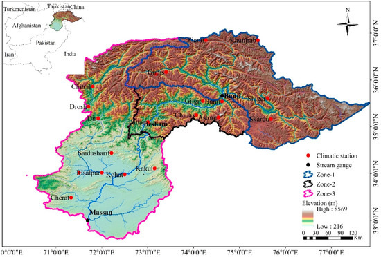
Figure 1.
Upper Indus basin.
3. Data Collection
The data of these stations were collected from Pakistan Surface-water Hydrology Project (SWHP), Water and Power Development Authority (WAPDA), and Pakistan Meteorological Department (PMD) for the period. Stream-flow measurement in UIB is of the WAPDA-SWHP project conceded starting in the 1960s with original records. All the hydrometric stations considered in this research are unregulated and reasonably free from land-use changes. Due to the wide variation in climate characteristics, the basin is divided into three distinct sub-zones known as the zone one (z1) having outlet Bunji, zone two (z2) having outlet Besham Qila, and zone three (z3) having outlet Massan. Three Hydraulic stations and 17 climatic stations (CS) were selected for the analysis. There are five climate and one hydrometric station in the z1, and three climate and one hydrometric stations in the z2, and nine climate and one hydrometric station in the z3 of the basin. The characteristics information of the selected is sites given in Table 1 and Table 2. The data of these sites were for period 1960 to 2012, 1969–2012, and 1972–2012, respectively, for zone 1, 2, and 3 (z1, z2, z3). There are five climate and one hydrometric station in the z1, three climate and one hydrometric stations in the z2, and nine climate and one hydrometric station in the z3 of the basin.

Table 1.
Hydrometric stations in UIB.
Table 2.
Climate stations in UIB.
As a norm with ANN and decomposition-based models, the whole data set is divided into training (weight adjustments) and testing (a different set of unseen data) to check the model applicability. In this study for zone one, out of a total of 50 years of data, the first 30 years (1960–1992, 60%) were used for model training and the remaining 20 years (1993–2012, 40%) for model testing. For zone two out of a total of 43 years of data, the first 26 years (1969–1995, 60%) were used for model training and the remaining 17 years (1996–2012, 40%) for model testing. Similarly, for zone three out of a total of 40 years of data, the first 24 years (1972–1996, 60%) were used for model training and the remaining 16 years (1997–2012, 40%) were used for model testing. Before going for a training phase, all datasets were normalized between 0 and 1 in order to equalize the relative significance of the inputs.
The following relationship was used to achieve the formula below.
4. Methodology
4.1. Artificial Neural Networks
4.1.1. Feed Forward Backpropagation
Up to now, artificial intelligence (AI) methods have been used and applied with a large number of achievements. One of the classic AI models is feed forward neural networks (FFNNs). Among other neural networks, the feed-forward neural network using error back propagation (BP) as a training algorithm has been recognized as the most famous AI model and is often applied in hydrological modeling. As a data-driven model, the three-layer BP neural networks have been proven that they do not require detail inherent information about the real system and can theoretically approximate any continuous nonlinear function producing high accuracy results under the condition of appropriate weight sets and a reasonable structure. Additionally, it has many superior features such as: self-learning, self-adaptability, highly robust, and fault tolerant [92]. Hence, BP is an acceptable and efficient approach for modeling complex input-output interactions in hydrological time series prediction.
The architecture of a general three-layer BP is shown in Figure 2. Since it can be seen from Figure 2, BP consists of one input layer, one output layer, and one hidden layer with numerous non-linear, random, and compact interconnected processing nodes called neurons. The establishment of the BP model includes two phases. The first is forward propagation in which the input vectors are propagated in the forward direction from the input to the output layer. The second is that the error propagated in the backward direction to update the weights for minimizing the global errors. These two phases repeat until the error between calculated output and the desired output is small enough.
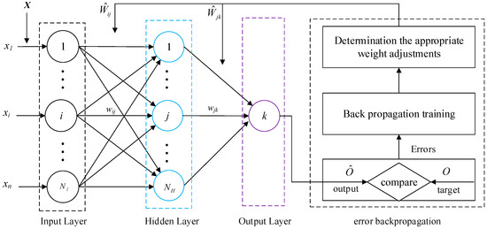
Figure 2.
The general structure of BP.
A brief procedure of the traditional BP is displayed below. More detail information can be found in Reference [93].
Phase 1: Forward Propagation
- (1)
- Calculate outputs for all hidden layer units using normalized input-output data pairs.where f is an activation function, which is usually a sigmoid function, indicates the connection weight from the i-th input node to the j-th hidden unit, represents the bias of the j-th neuron, and y is the calculated output.
- (2)
- Calculate output values of the BP neural network.where represents the output value of the network, stands for the connection weight from the j-th hidden node to the k-th output node, is the bias of the neuron, and is the activation function of the output layer node.
- (3)
- Compute the global error E of the output node.where O represents the real output value.
Phase 2: Back propagation. In this stage, the weight adjustment formula is expressed below.
where represents the modification value of the weight and the constant is the learning rate of the network.
The traditional BP explores the most speed gradient descent correction method to adjust the weights and threshold, which leads to a low learning speed and local convergence. Hence, in this study, a famous improved learning algorithm known as Levenberg-Marquardt (LM) is adopted to accelerate the training and convergence. Due to this, the algorithm combines the advantages of the gradient descent method and the Quasi-Newton method to ensure the locally fast convergence speed and maintain better overall performance.
4.1.2. Radial Basis Function Neural Network
Radial basis function neural networks were developed in Reference [94]. They are a special type of neural network that takes a radial basis function as its activation function. Unlike the commonly used artificial neural networks, RBFNN networks have fast learning speed and do not suffer problems like local minima. Hence, RBFNN networks have attracted considerable attention and have been widely applied in many other fields [95,96,97,98]. RBFNN is a classic three-layer feed forward propagated neural network. Its activation functions in the hidden layer are a set of radial symmetrical kernel functions. A general architecture of a three-layered RBFNN is shown in Figure 3. Clearly, it is generally composed of three layers: an input layer, a single hidden layer with several nonlinear processing units, and an output layer. For a set of the input vector , the output of RBFNN is calculated in terms of Equation (5).
where m is the dimension of input vectors, h is the number of hidden nodes, are the associate weights from the i-th node in the hidden layer to output layer, indicates the Euclidean norm, represents the RBF center vector in the input vector, and denotes the nonlinear activation function, which usually adopts a normalized Gaussian function. A normalized Gaussian function is defined in the following expression.
where represents the radius of the i-th unit.
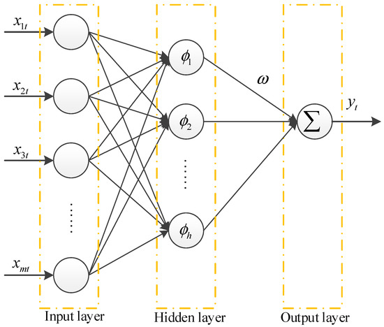
Figure 3.
The general structure of RBF.
The development of RBFNN includes determining the number of nodes in the hidden layer. Next, three parameters including center , radius , and weight need to be determined for each neuron in the hidden layer in order to obtain the desired output of RBFNN.
4.2. Discrete Wavelet Transform
The wavelet transform is a powerful mathematical tool for nonstationary time series analysis. It usually can be divided into two typical types: continuous wavelet transform (CWT) and discrete wavelet transform (DWT). The continuous wavelet for a time series is obtained through translation and expansion of a mother wavelet .
where factor a and b, respectively, represent the temporal scale and time translation and is the complex conjugate of the wavelet function . is a wavelet coefficient of the continuous wavelet. For the practical application in hydrology, the observed hydrological time series generally is non-linear, non-stationary discrete signals. Hence, the DWT, in which the wavelets are discretely sampled, is adopted and defined as the formula below.
where is a discrete wavelet coefficient with scale and location . N is an integer power of 2, i.e., .
During the DWT process, the original time series is passed through high-pass and low-pass filters and then decomposed into an approximation component A1 and a detail component D1 after the A1 is further decomposed into another approximation component A2 and a detail component D2. This procedure is stopped until it reached a suitable decomposition level (L). At the end of this decomposing procedure, the original time series x(t) can be expressed by several details (D) and one approximation (A) component.
4.3. Empirical Mode Decomposition and Ensemble Empirical Mode Decomposition
The empirical mode decomposition (EMD) is suitable for the analysis of nonlinear and non-stationary time series. It can decompose a given signal into several intrinsic mode functions (IMFs) and one residue. Every IMF must satisfy the following two conditions: the first one is that the number of extrema within the whole time series must equal to the number of zero crossings or differ at most by one. The other is that the average value of the upper and lower must be zero at any point. On the basis of the above conditions, a time series x(t) decomposing by the EMD method can be expressed as the equation below.
where stands for the IMFs, m is the number of IMF, and represents the residual series.
During the EMD procedure, the extreme points of the time series are first determined and then cubic spline interpolation is applied to construct the upper and lower envelopes with all the local maximum and minimum values, respectively. It has been proven that the selection of extremes is sensitive to abnormal points in the original data and consequently affects the calculation of the envelopes. Hence, the derived envelopes may be the mixtures of envelopes from the real signal and abnormal points. In this way, the mode mixing phenomenon occurs.
In order to eliminate the mode mixing problem, ensemble empirical mode decomposition (EEMD) has been developed [99]. The essence of EEMD method is adding white noise, which falls uniformly in the entire time-frequency space to assist the EMD method and facilitate a natural separation of the frequency scales as well as reduce the occurrence of mode mixing. The entire procedure of the EEMD approach can be briefly described as:
- (1)
- Initialize ensemble number En and the amplitude of the additional white noise.
- (2)
- Add a white noise series to the original time series and then a new time series can be obtained.
- (3)
- Decompose the new time series into several IMFs using a traditional EMD method.where and , respectively, stand for the j-th IMF and residual series during the i-th experiment.
- (4)
- Repeat steps (2) and (3) En times and add different white noise series at each time (In this work, En = 20 times).
- (5)
- Calculate the ensemble average values of all IMF components and residue components as the final result.
4.4. Decomposition of Original Data
4.4.1. Application of DWT
DWT is applied to decompose the original streamflow, precipitation, and temperature data for each zone 1, 2, and 3 and decomposed sub-series for each zone 1, 2, and 3 are shown in Figure 4, Figure 5 and Figure 6, respectively. The decomposition process is suggested by [100,101] and is used to obtain the subseries of two decomposition levels, which is recommended. Selecting an appropriate mother wavelet is critical to obtain a better wavelet hybrid model. For hydrological series, it is very difficult to obtain the best mother wavelet due to its non-linearity characteristic [102]. Hence, the Daubechies wavelet with three vanishing moments (db3), which is an irregular mother wavelet, has a very high number of vanishing moments for a given support width. Two decomposition levels series of approximations (A) and details (D) through the high-pass and low-pass filter coefficients of the chosen db3 are displayed in Figure 4, Figure 5 and Figure 6, respectively. Each subseries may represent a special level of the temporal characteristics of the original time series. It can be seen from Figure 4, Figure 5 and Figure 6 that the high-frequency decomposed component D1 is the most non-linear and disordered.
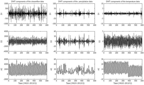
Figure 4.
Zone One: streamflow, precipitation, and temperature data are decomposed by DWT.
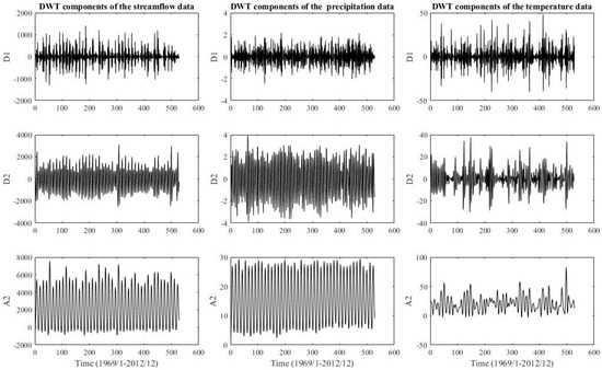
Figure 5.
Zone Two: streamflow, precipitation, and temperature data are decomposed by DWT.
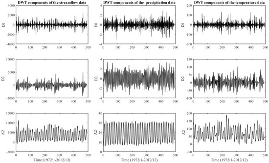
Figure 6.
Zone Three: streamflow, precipitation, and temperature data are decomposed by DWT.
4.4.2. Applying EEMD
The EEMD technique is applied to decompose all three zones of original streamflow, precipitation, and temperature into several independent IMFs and one residue, respectively. The IMF1, IMF2 IMF3, and IMF4 components are shown in Figure 7, Figure 8 and Figure 9. The original time series is decomposed into four independent IMF components in the order from the highest frequency to the lowest frequency and one residue component, respectively. The IMFs represent changing frequencies, amplitudes, and wavelengths, which can be seen in Figure 7, Figure 8 and Figure 9 and IMF4 is the minimum amplitude, lowest frequency, and the longest wavelength. The other IMF components increase in the amplitude and frequency and decrease in the wavelength. The last residue is a mode slowly changing the long-term average. The residue component indicates the overall trend of streamflow, precipitation, and temperature time series. Therefore, the EEMD decomposition characterizes a physically meaningful decomposition. Although the decomposition is made for each instant in the spatial dimension and is totally independent of the other instants, it is physically consistent with the decompositions at neighboring instants [103]. Therefore, the decomposition can be helpful to transform non-linear and non-stationary time series to stationary time series and can be useful to improve prediction performance [104].
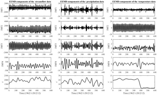
Figure 7.
Zone One: streamflow, precipitation, and temperature data are decomposed by EEMD.
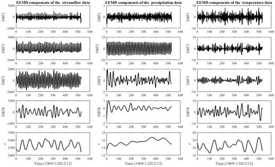
Figure 8.
Zone Two: streamflow, precipitation, and temperature data are decomposed by EEMD.
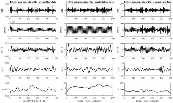
Figure 9.
Zone Three: streamflow, precipitation, and temperature data are decomposed by EEMD.
4.5. The Establishment of the Hybrid Artificial Neural Network
In this study, two decomposing methods (DWT and EEMD) and two types of neural networks (BP and RBF) are combined into four different hybrid models: DWT-BP, DWT-RBF, EEMD-BP, and EEMD-RBF. The establishment of DWT and EEMD based ANN models is as follows. The first appropriate input vector for hybrid models should be determined according to the auto-correlation function (ACF) and the cross-correlation function (PACF). On the basis of the autocorrelation function and the cross-correlation function of streamflow, temperature, and precipitation, the oriented results for each zone 1, 2, and 3 are shown in Figure 10, Figure 11 and Figure 12, respectively. Then each input factor is decomposed by DWT into L+1 subseries after the determination of a suitable decomposition level L and an appropriate mother wavelet. Afterward, all these subseries are taking as input for ANN to predict a monthly stream flow.
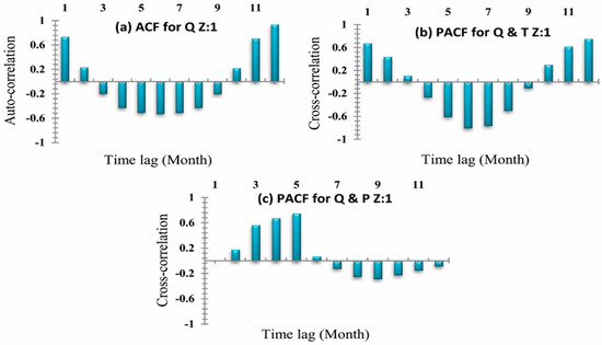
Figure 10.
Zone One (a) Auto-correlation coefficients for stream-flow. (b) Cross-correlation coefficient for stream-flow and temperature. (c) Cross-correlation coefficient for stream-flow and rainfall.
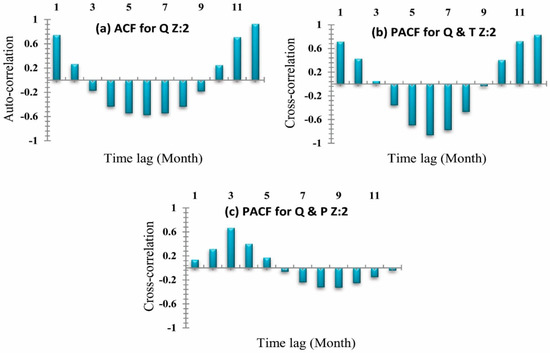
Figure 11.
Zone Two (a) Auto-correlation coefficients for stream-flow. (b) Cross-correlation coefficient for stream-flow and temperature. (c) Cross-correlation coefficient for stream-flow and rainfall.
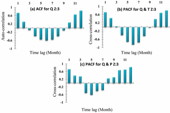
Figure 12.
Zone Three (a) Auto-correlation coefficients for stream-flow. (b) Cross-correlation coefficient for stream-flow and temperature. (c) Cross-correlation coefficient for stream-flow and rainfall.
Generally, the accuracy of DWT-based models is sensitive to the given mother wavelet. However, there is no specific method to determine a suitable mother wavelet. In the present study, an irregular mother wavelet, the Daubechies wavelet with three vanishing moments (db3), is used. The decomposition level L is calculated by the below equation.
where N is the total number of samples.
The EEMD-based ANN models are developed in combination with EEMD instead of DWT. After selecting a suitable set of input, an appropriate ensemble number En and white noise amplitude need to be determined. The subsequent steps are similar to the DWT-based ANN models. A flowchart of these four hybrid neural network models is presented in Figure 13.
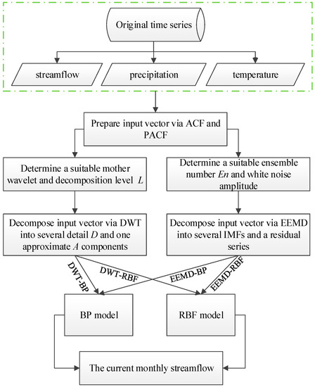
Figure 13.
The flowchart of the hybrid models.
5. Results and Discussions
This section may be divided by subheadings. It should provide a concise and precise description of the experimental results, their interpretation, and the experimental conclusions that can be drawn.
5.1. Model Development
In this research, at UIB, applied models such as FFBP, RBFNN, DWT-FFBP, DWT-RBFNN, EEMD-FFBP, and EEMD-RBFNN debated in Section 4 are assessed for predicting 1-month-ahead stream- flow. Using different input combinations, twelve models FFBP-Q, FFBP-QTP, RBFNN-Q, RBFNN-QTP, DWT-FFBP-Q, DWT-FFPB-QTP, DWT-RBFNN-Q, DWT-RBFNN-QTP, EEMD-FFBP-Q, EEMD-FFBP-QTP, EEMD-RBFNN-Q, and EEMD-RBFNN-QTP are developed in this research study. All developed models and their corresponding inputs for zone 1, 2, and 3 are given in Table 3, Table 4 and Table 5, respectively.
Table 3.
Models and their corresponding inputs for zone one.
Table 4.
Models and their corresponding inputs for zone two.
Table 5.
Models and their corresponding inputs for zone three.
5.2. Model Performance Evaluation
To qualitatively evaluate the forecast ability of all models, five main criteria are applied. These indices are correlation coefficient (R), root mean square errors (RMSE), Nash-Sutcliffe Efficiency (NSE), mean absolute percentage error (MAPE), and mean absolute errors (MAE). They are defined by using the equations below.
where and represent the observed and computed streamflow, is the average of the observed streamflow, and N is the total number of samples.
5.3. Results Analysis
The aim of this research was to find an appropriate model to predict discharge at UIB. This study will help find the flood magnitudes of different seasons at the proposed hydropower (Pattan Hydropower, Thakot Hydropower, Dasu Hydropower, Diamer-Basha Hydropower, Bunji Hydropower) of the upper Indus basin. The basin is divided into three distinct sub-zones such as zone one (z1), zone two (z2), and zone three (z3). The forecast stations for each zone were Bunji, Besham Qila, and Massan respectively. To predict the discharge at z1 monthly rainfall data and temperature data of 5 meteorological stations and monthly runoff data of 50 years (1960 to 2012) were collected from Bunji for z2 monthly rainfall data and temperature data of 3 meteorological stations and monthly runoff data of 43 years (1969–2012) were collected from Besham Qila hydrometric station and for z3 monthly rainfall data and temperature data of 9 meteorological stations and monthly runoff data of 40 years (1972–2012) were collected from Besham Qila hydrometric station and for z3. To reduce the model input data requirements and simplification, the average rainfall and temperature data of all the 5, 3, and 9 meteorological stations were used for each zone, respectively, as debated in Section 3. Two types of neural networks (BP and RBF) are coupled with two types of decomposition methods to form four different hybrid models: DWT-BP, DWT-RBF, EEMD-BP, and EEMD-RBF. By using the monthly average streamflow (Q), monthly average temperature (T), and monthly average precipitation (P) as inputs with four basic hybrid models give 12 new hybrid models: FFBP-Q, FFBP-QTP, RBFNN-Q, RBFNN-QTP, DWT-FFBP-Q, DWT-FFPB-QTP, DWT-RBFNN-Q, DWT-RBFNN-QTP, EEMD-FFBP-Q, EEMD-FFBP-QTP, EEMD-RBFNN-Q, and EEMD-RBFNN-QTP, which were applied at forecast stations Bunji, Besham Qila, and Massan, respectively. Results for this research can be described in three steps for each zone (z1, z2, and z3) simultaneously on the basis of applied performance indices which can be seen in Table 6, Table 7, Table 8, Table 9, Table 10 and Table 11 and flow the hydrograph between original and simulated time series including 1: on the basis of inputs, 2: comparison between AI based models, 3: comparison between Hybrid Models, 4: Inter-comparison of each applied models Table 6, Table 8 and Table 10 reports the performance of ANN-based models (BP and RBF) and hybrid models DWT-BP, DWT-RBF, EEMD-BP, and EEMD-RBF in each zone (z1, z2, and z3) for the calibration period while Table 7, Table 9 and Table 11 are reporting performances for the validation period, respectively. The correlation coefficient (R), root mean square errors (RMSE), Nash-Sutcliffe Efficiency (NSE), mean absolute percentage error (MAPE), and mean absolute errors (MAE) statistical criteria were selected to assess the predictive capability of all applied models. Performance evaluation criteria indicates that FFBP-QTP, RBFNN-QTP, DWT-FFPB-QTP, DWT-RBFNN-QTP, EEMD-FFBP-QTP, and EEMD-RBFNN-QTP models, which includes (Q, T, and P) as input, was the best as compared to FFBP-Q, RBFNN-Q, DWT-FFBP-Q, DWT-RBFNN-Q, EEMD-FFBP-Q, EEMD-RBFNN-Q in which only (Q) is used for each zone (z1, z2, and z3) shown in Table 6, Table 7, Table 8, Table 9, Table 10 and Table 11, respectively. Similar results are indicated in flow hydrographs that models which possess (Q, T, and P) simulate the observed time series much better as compared to only (Q) input models. It confirms that the use of precipitation and temperature can increase modeling accuracy for each zone (z1, z2, and z3) [105], as shown in Figure 14, Figure 15 and Figure 16, respectively.
Table 6.
Performance evaluation of the applied models for Zone One during the calibration period.
Table 7.
Performance evaluation of the applied models for zone one during the validation period.
Table 8.
Performance evaluation of the applied models for zone two during the calibration period.
Table 9.
Performance evaluation of the applied models for zone two during the validation period.
Table 10.
Performance evaluation of the applied models for zone three during the calibration period.
Table 11.
Performance evaluation of the applied models for zone three during the validation period.
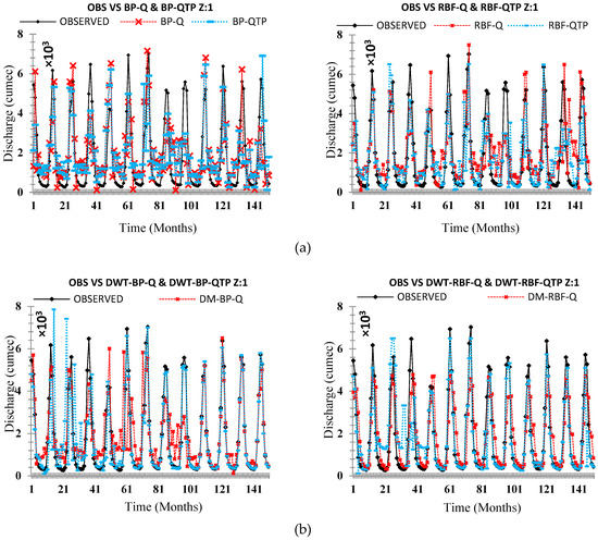
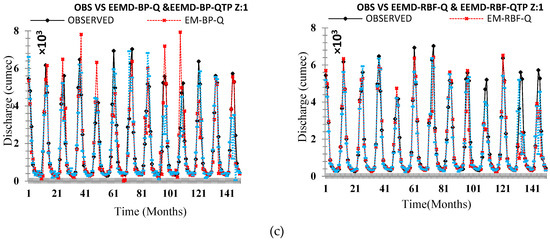
Figure 14.
Comparison of the originally observed streamflow and the simulated runoff hydrograph Zone One (a) OBS VS ANN (Q & QTP) Inputs, (b) OBS VS ANN-DWT (Q & QTP) Inputs, and (c) OBS VS ANN-EEMD (Q & QTP) Inputs.
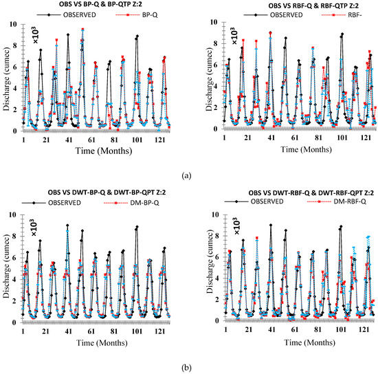
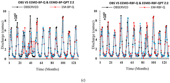
Figure 15.
Comparison of the originally observed streamflow and the simulated runoff hydrograph Zone Two (a) OBS VS ANN (Q & QTP) Inputs, (b) OBS VS ANN-DWT (Q & QTP) Inputs, and (c) OBS VS ANN-EEMD (Q & QTP) Inputs.
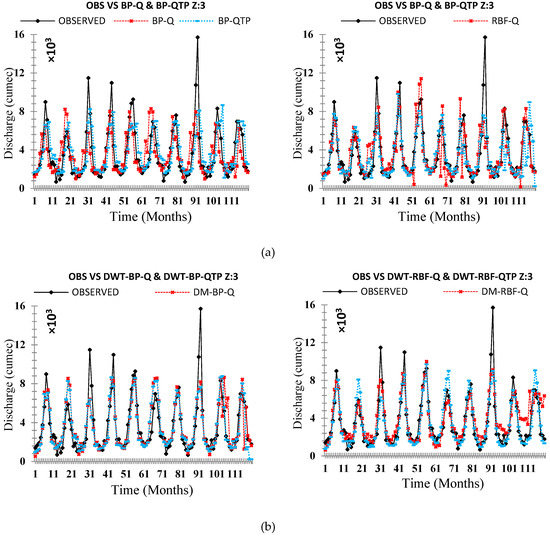
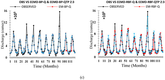
Figure 16.
Comparison of the originally observed streamflow and the simulated runoff hydrograph Zone Three (a) OBS VS ANN (Q & QTP) Inputs, (b) OBS VS ANN-DWT (Q & QTP) Inputs, and (c) OBS VS ANN-EEMD (Q & QTP) Inputs.
On an individual basis, applied neural networks (FFBP-NN, RBF-NN) led to significant results. The performance evaluation criteria indicate that the RBF neural network holds superiority on the FFBP neural network. All applied statistical indices (R), (RMSE), (NSE), (MAPE), and (MAE) shows better results for RBF neural networks for each zone (z1, z2, and z3) shown in Table 7, Table 9 and Table 11, respectively. The validation hydrograph for simulated (FFBP-NN, RBF-NN) versus observed time series shows RBF neural network was the best at picking the range of values for each zone (z1, z2, and z3), as shown in Figure 14, Figure 15 and Figure 16, respectively. However, back-propagation has potential aptitudes. It occurs from some problems that can lead to complications during calibration periods such as long, ambiguous training process, network paralysis, and local minima, which is shown in Table 6, Table 8 and Table 10, respectively, for each zone (z1, z2, and z3) that (FFBP-NN) has shown recessive outcomes as compared to (RBF-NN).
The original time series data were decomposed by DWT and EEMD methods to established four hybrid models: DWT-BP, DWT-RBF, EEMD-BP, and EEMD-RBF, which were applied in each zone (z1, z2, and z3). DWT and EEMD have significantly improved the results of individual AI-based models but, among DWT and EEMD methods, the models that are coupled with DWT such as DWT-FFBP and DWT-RBFNN were shown less significant models as compared to those which were coupled by EEMD such as EEMD-FFBP and EEMD-RBFNN. Results showed that, on an individual basis, the RBF neural network is performing better as compared to the FFBP neural network similarly to the hybrid model EEMD-RBFNN, which is performing better than DWT-FFBP, DWT-RBFNN, and EEMD-FFBP. Both performance indices and flow hydrographs are verifying that EEMD-based hybrid models are more powerful models to simulate the original time series of each zone (z1, z2, and z3), which is shown in Table 6, Table 7, Table 8, Table 9, Table 10 and Table 11 and Figure 14, Figure 15 and Figure 16, respectively.
To disclose the outcome of different decomposing methods on model precision, a complete analysis needs to be made based on Table 7, Table 9 and Table 11. Relate FFBP-QTP, RBFNN-QTP, DWT- DWT-FFPB-QTP, DWT-RBFNN-QTP, EEMD-FFBP-QTP, and EEMD-RBFNN-QTP in each zone (z1, z2, and z3). All of these are optimum models. Therefore, models coupled with decomposition techniques (DWT and EEMD) contribute with high precision than the single AI-based model. EEMD-RBF-QTP increases the accuracy of prediction further than DWT-FFPB-QTP, DWT-RBFNN-QTP, and EEMD-FFBP-QTP in validation periods. For that reason, application of decomposition techniques gives an improvement in non-linear time series forecasting. The decomposing technique EEMD is more suitable than DWT for monthly streamflow modeling for each zone (z1, z2, and z3) of UIB, as shown in Table 6, Table 7, Table 8, Table 9, Table 10 and Table 11 and Figure 14, Figure 15 and Figure 16, respectively.
5.4. Peak Value Analysis
To confirm the previous results stated in Section 5.3, all models: FFBP-Q, FFBP-QTP, RBFNN-Q, RBFNN-QTP, DWT-FFBP-Q, DWT-FFPB-QTP, DWT-RBFNN-Q, DWT-RBFNN-QTP, EEMD-FFBP-Q, EEMD-FFBP-QTP, EEMD-RBFNN-Q, and EEMD-RBFNN-QTP were applied to test the precision rate during the flood season (May–October). This is considered to be the flood season in UIB because, during this period, the temperature gets high and the melting glacier effects the discharge with a greater ability. In this study, 20% is considered as a reasonable and acceptable relative error and results of FFBP-Q, FFBP-QTP, RBFNN-Q, RBFNN-QTP, DWT-FFBP-Q, DWT-FFPB-QTP, DWT-RBFNN-Q, DWT-RBFNN-QTP, EEMD-FFBP-Q, EEMD-FFBP-QTP, EEMD-RBFNN-Q, and EEMD-RBFNN-QTP in the validation period are shown in Figure 17, Figure 18 and Figure 19 for each zone (z1, z2, and z3). DWT-FFPB-QTP, DWT-RBFNN-QTP, EEMD-FFBP-QTP, and EEMD-RBFNN-QTP approximate the observed streamflow better than single ANN models and hybrid models with only (Q) components. Percentage of standard forecasts (SF), which is known as an eligible rate (ER), is shown in Table 12, Table 13 and Table 14 for each zone (z1, z2, and z3), respectively. The results indicate that EEMD-RBFNN-QTP increases the eligible rate (ER) from 67% of DWT-RBFNN-QTP to 82% at zone one (z1). The zone increases from 85% to 91% and similarly for zone three (z3). EEMD-RBFNN-QTP dominates with 89% eligible rate (ER) to 76% of DWT-RBFNN-QTP. Therefore, EEMD-RBFNN-QTP attains the highest predicting capacity for the peak value streamflow.
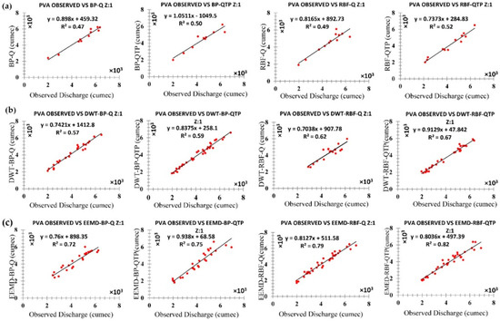
Figure 17.
Monthly streamflow estimations for peak values in the flood season Zone One (a) OBS VS ANN (Q & QTP) Inputs, (b) OBS VS ANN-DWT (Q & QTP) Inputs, and (c) OBS VS ANN-EEMD (Q & QTP) Inputs.
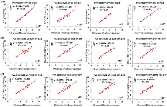
Figure 18.
Monthly streamflow estimations for peak values in the flood season Zone Two (a) OBS VS ANN (Q & QTP) Inputs, (b) OBS VS ANN-DWT (Q & QTP) Inputs, and (c) OBS VS ANN-EEMD (Q & QTP) Inputs.
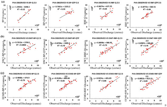
Figure 19.
Monthly streamflow estimations for peak values during the flood season Zone Three (a) OBS VS ANN (Q & QTP) Inputs, (b) OBS VS ANN-DWT (Q & QTP) Inputs and, (c) OBS VS ANN-EEMD (Q & QTP) Inputs.
Table 12.
An acceptable rate of forecasting for peak values during the flood season (May–October) for Zone One.
Table 13.
An acceptable rate of forecasting for peak values during the flood season (May–October) for Zone Two.
Table 14.
An acceptable rate of forecasting for peak values during the flood season (May–October) for Zone Three.
6. Conclusions
Enhancing the precision rate of hydrological forecasting is very important for UIB and an exact flood prediction along with the right lead time can provide future precautions of the forthcoming flood event. Complete safety is impossible, but, by timely and accurate predictions of flood crests, flood magnitude, and flood duration, huge amounts of money and countless lives can be saved. Bunji, Besham Qila, and Massan stations are the forecast station for this study located at the UIB. These indices are the correlation coefficient (R), root mean square errors (RMSE), Nash-Sutcliffe Efficiency (NSE), mean absolute percentage error (MAPE), and mean absolute errors (MAE), which are used as performance evaluation criteria. The results were also presented as flow hydrographs between observed and simulated time series for each zone (z1, z2, and z3).
The conclusion of this research is as follows:
- The results are improved by adding the temperature and precipitation to the model as input. All models that include (QTP) as input has performed with great accuracy. FFBP-QTP, RBFNN-QTP, DWT-FFPB-QTP, DWT-RBFNN-QTP, EEMD-FFBP-QTP, and EEMD-RBFNN-QTP are the best performing models based on inputs.
- Applied neural networks such as (FFBPNN and RBFNN), RBFNN has shown better results as compared to FFBBNN. Therefore, on an individual basis, RBFNN-QTP is considered to be a better model.
- Among applied decomposition methods (DWT and EEMD), EEMD has performed well in all cases. Both DWT and EEMD have significantly improved the results of individual-based neural network models.
- In comparison, it is revealed that, among FFBP-Q, FFBP-QTP, RBFNN-Q, RBFNN-QTP, DWT-FFBP-Q, DWT-FFPB-QTP, DWT-RBFNN-Q, DWT-RBFNN-QTP, EEMD-FFBP-Q, EEMD-FFBP-QTP, EEMD-RBFNN-Q, and EEMD-RBFNN-QTP EEMD-RBFNN-QTP gives the greatest accuracy.
- The EEMD method has the precision of monthly streamflow prediction. Meanwhile, it can be seen that EEMD-FFBP-QTP overtakes EEMD-RBF-QTP in terms of the performance indices and flow hydrograph.
- For peak value estimation during the flood season, EEMD-RBFNN-QTP increases the eligible rate (ER) from 67% of DWT-RBFNN-QTP to 82% at zone one (z1). For the zone two (z2) it increases from 85% to 91% and similarly for zone three (z3), EEMD-RBFNN-QTP dominates with an 89% eligible rate (ER) to 76% of DWT-RBFNN-QTP.
- Therefore, the optimum model for this research is EEMD-RBFNN-QTP and it attains the highest predicting capacity in all cases and all zones of UIB.
- Limitations and future directions: The quality and the quantity of data available are the success factors of an ANN application and this requirement cannot be easily met. Even though long historic records are accessible, we are not sure that circumstances stayed consistent over this period. Another major limitation of ANNs is the lack of physical concepts and relations. This makes the resulting ANN structure more complicated. Future investigations can be done on a large-deep foundation pit of a hydraulic structure rehabilitation program across the River Indus in the Punjab province of Pakistan. Construction and rehabilitation programs of hydraulic river structures invariably involve structural activities in the riverbed and efficient dewatering of construction sites always plays a crucial role for undisturbed structural works.
Author Contributions
M.T. and N.S. designed this experiment. M.T. wrote the whole paper. I.A. analyzed the data. X.D. reviewed drafts of the paper. J.Z. contributed reagents/materials/analysis tools. X.D. and M.T. designed the software and performed the computation work.
Funding
This study was supported by the State Key Program of National Natural Science of China (51239004), the National Natural Science Foundation of China (51309105, 40701024) and the application research of hydro-meteorological major key technology funded by the Power Construction Corporation of China (DJ-ZDZX-2016-02).
Acknowledgments
This study was supported by the State Key Program of National Natural Science of China (51239004), the National Natural Science Foundation of China (51309105, 40701024) and the application research of hydro-meteorological major key technology funded by the Power Construction Corporation of China (DJ-ZDZX-2016-02).
Conflicts of Interest
The authors declare no conflict of interest.
References
- Tayyab, M.; Zhou, J.; Zeng, X.; Chen, L.; Ye, L. Optimal application of conceptual rainfall-runoff hydrological models in the Jinshajiang River basin, China. Remote Sens. GIS Hydrol. Water Resour. 2015, 368, 227–232. [Google Scholar] [CrossRef]
- Fotovatikhah, F.; Herrera, M.; Shamshirband, S.; Chau, K.-W.; Ardabili, S.F.; Piran, M.J. Survey of computational intelligence as basis to big flood management: Challenges, research directions and future work. Eng. Appl. Comput. Fluid Mech. 2018, 12, 411–437. [Google Scholar] [CrossRef]
- Penman, H.L. Weather, plant and soil factors in hydrology. Weather 1961, 16, 207–219. [Google Scholar] [CrossRef]
- Dariane, A.B.; Karami, F. Deriving hedging rules of multi-reservoir system by online evolving neural networks. Water Resour. Manag. 2014, 28, 3651–3665. [Google Scholar] [CrossRef]
- Boughton, W.; Droop, O. Continuous simulation for design flood estimation—A review. Environ. Model. Softw. 2003, 18, 309–318. [Google Scholar] [CrossRef]
- Taormina, R.; Chau, K.W.; Sivakumar, B. Neural network river forecasting through baseflow separation and binary-coded swarm optimization. J. Hydrol. 2015, 529, 1788–1797. [Google Scholar] [CrossRef]
- Cheng, C.T.; Chau, K.W. Flood control management system for reservoirs. Environ. Model. Softw. 2004, 19, 1141–1150. [Google Scholar] [CrossRef]
- Bürger, C.M.; Kolditz, O.; Fowler, H.J.; Blenkinsop, S. Future climate scenarios and rainfall–runoff modelling in the Upper Gallego catchment (Spain). Environ. Pollut. 2007, 148, 842–854. [Google Scholar] [CrossRef] [PubMed]
- Chen, L.; Sun, N.; Zhou, C.; Zhou, J.; Zhou, Y.; Zhang, J.; Zhou, Q. Flood forecasting based on an improved extreme learning machine model combined with the backtracking search optimization algorithm. Water 2018, 10, 1362. [Google Scholar] [CrossRef]
- Zhou, C.; Sun, N.; Chen, L.; Ding, Y.; Zhou, J.; Zha, G.; Luo, G.; Dai, L.; Yang, X. Optimal operation of cascade reservoirs for flood control of multiple areas downstream: A case study in the Upper Yangtze River basin. Water 2018, 10, 1250. [Google Scholar] [CrossRef]
- Tayyab, M.; Zhou, J.; Dong, X.; Ahmad, I.; Sun, N. Rainfall-runoff modeling at Jinsha River basin by integrated neural network with discrete wavelet transform. Meteorol. Atmos. Phys. 2017, 1–11. [Google Scholar] [CrossRef]
- Seo, Y.; Kim, S.; Singh, V.P. Machine learning model coupled with variational mode decomposition: A new approach for modeling daily rainfall-runoff. Atmosphere 2018, 9, 251. [Google Scholar] [CrossRef]
- Wu, C.L.; Chau, K.W. Rainfall–runoff modeling using artificial neural network coupled with singular spectrum analysis. J. Hydrol. 2011, 399, 394–409. [Google Scholar] [CrossRef]
- Barge, J.T.; Sharif, H.O. An ensemble empirical mode decomposition, self-organizing map, and linear genetic programming approach for forecasting river streamflow. Water 2016, 8, 247. [Google Scholar] [CrossRef]
- Carlson, R.F.; Maccormick, A.J.A.; Watts, D.G. Application of linear random models to four annual streamflow series. Water Resour. Res. 1970, 6, 1070–1078. [Google Scholar] [CrossRef]
- Yu, X.; Zhang, X.; Qin, H. A data-driven model based on fourier transform and support vector regression for monthly reservoir inflow forecasting. J. Hydro-Environ. Res. 2017, 18, 12–24. [Google Scholar] [CrossRef]
- Sudheer, K.P.; Gosain, A.K.; Rangan, D.M.; Saheb, S.M. Modelling evaporation using an artificial neural network algorithm. Hydrol. Process. 2002, 16, 3189–3202. [Google Scholar] [CrossRef]
- Box, G.E.; Jenkins, G.M. Time Series Analysis: Forecasting and Control, Rev. ed; Holden-Day: San Francisco, CA, USA, 1976; Volume 31, pp. 238–242. [Google Scholar]
- Karami, F.; Dariane, A.B. Optimizing signal decomposition techniques in artificial neural network-based rainfall-runoff model. Int. J. River Basin Manag. 2017, 15, 1–8. [Google Scholar] [CrossRef]
- Ghorbani, M.A.; Kazempour, R.; Chau, K.-W.; Shamshirband, S.; Ghazvinei, P.T. Forecasting pan evaporation with an integrated artificial neural network quantum-behaved particle swarm optimization model: A case study in Talesh, Northern Iran. Eng. Appl. Comput. Fluid Mech. 2018, 12, 724–737. [Google Scholar] [CrossRef]
- Cheng, C.T.; Wu, X.Y.; Chau, K.W. Multiple criteria rainfall-runoff model calibration using a parallel genetic algorithm in a cluster of computers. Hydrol. Sci. J. 2005, 50, 1069–1087. [Google Scholar] [CrossRef]
- Chau, K.W. Use of meta-heuristic techniques in rainfall-runoff modelling. Water 2017, 9, 186. [Google Scholar] [CrossRef]
- Box, G.E.P.; Jenkins, G.M.; Reinsel, G.C. Time Series Analysis: Forecasting and Control, 4th ed.; John Wiley & Sons, Inc.: Hoboken, NJ, USA, 2008; p. 14. [Google Scholar]
- Chen, H.L.; Rao, A.R. Linearity analysis on stationary segments of hydrologic time series. J. Hydrol. 2003, 277, 89–99. [Google Scholar] [CrossRef]
- Gilroy, K.L.; Mccuen, R.H. A nonstationary flood frequency analysis method to adjust for future climate change and urbanization. J. Hydrol. 2012, 414, 40–48. [Google Scholar] [CrossRef]
- Zhang, Q.; Gu, X.; Singh, V.P.; Xiao, M.; Chen, X. Evaluation of flood frequency under non-stationarity resulting from climate indices and reservoir indices in the East River basin, China. J. Hydrol. 2015, 527, 565–575. [Google Scholar] [CrossRef]
- Milly, P.; Julio, B.; Malin, F.; Robert, M.H.; Zbigniew, W.K.; Dennis, P.L.; Ronald, J.S. Stationarity is dead. Science 2008, 319, 573–574. [Google Scholar] [CrossRef] [PubMed]
- Wang, W.C.; Chau, K.W.; Cheng, C.T.; Qiu, L. A comparison of performance of several artificial intelligence methods for forecasting monthly discharge time series. J. Hydrol. 2009, 374, 294–306. [Google Scholar] [CrossRef]
- Kisi, O. Streamflow forecasting and estimation using least square support vector regression and adaptive neuro-fuzzy embedded fuzzy c-means clustering. Water Resour. Manag. 2015, 29, 5109–5127. [Google Scholar] [CrossRef]
- Bai, Y.; Chen, Z.; Xie, J.; Li, C. Daily reservoir inflow forecasting using multiscale deep feature learning with hybrid models. J. Hydrol. 2016, 532, 193–206. [Google Scholar] [CrossRef]
- Dariane, A.B.; Farhani, M.; Azimi, S. Long term streamflow forecasting using a hybrid entropy model. Water Resour. Manag. 2018, 32, 1439–1451. [Google Scholar] [CrossRef]
- Abdellatif, M.E.; Osman, Y.Z.; Elkhidir, A.M. Comparison of artificial neural networks and autoregressive model for inflows forecasting of roseires reservoir for better prediction of irrigation water supply in Sudan. Int. J. River Basin Manag. 2015, 13, 203–214. [Google Scholar] [CrossRef]
- Lin, G.F.; Wu, M.C. An RBF network with a two-step learning algorithm for developing a reservoir inflow forecasting model. J. Hydrol. 2011, 405, 439–450. [Google Scholar] [CrossRef]
- Coulibaly, P.; Anctil, F.; Bobée, B. Daily reservoir inflow forecasting using artificial neural networks with stopped training approach. J. Hydrol. 2000, 230, 244–257. [Google Scholar] [CrossRef]
- Sattari, M.T.; Yurekli, K.; Pal, M. Performance evaluation of artificial neural network approaches in forecasting reservoir inflow. Appl. Math. Model. 2012, 36, 2649–2657. [Google Scholar] [CrossRef]
- Lohani, A.K.; Goel, N.K.; Bhatia, K.K.S. Improving real time flood forecasting using fuzzy inference system. J. Hydrol. 2014, 509, 25–41. [Google Scholar] [CrossRef]
- Wang, W.; Nie, X.; Qiu, L. Support vector machine with particle swarm optimization for reservoir annual inflow forecasting. In Proceedings of the International Conference on Artificial Intelligence and Computational Intelligence, Sanya, China, 23–24 October 2010; pp. 184–188. [Google Scholar]
- Bengio, Y.; Courville, A.; Vincent, P. Unsupervised feature learning and deep learning: A review and new perspectives. arXiv, 2012; arXiv:1206.5538. [Google Scholar]
- Xu, J.; Chen, Y.; Li, W.; Nie, Q.; Song, C.; Wei, C. Integrating wavelet analysis and BPANN to simulate the annual runoff with regional climate change: A case study of Yarkand River, Northwest China. Water Resour. Manag. 2014, 28, 2523–2537. [Google Scholar] [CrossRef]
- Sattari, M.T.; Apaydin, H.; Ozturk, F. Flow estimations for the Sohu Stream using artificial neural networks. Environ. Earth Sci. 2012, 66, 2031–2045. [Google Scholar] [CrossRef]
- Yilmaz, A.G.; Imteaz, M.A.; Jenkins, G. Catchment flow estimation using artificial neural networks in the mountainous Euphrates basin. J. Hydrol. 2011, 410, 134–140. [Google Scholar] [CrossRef]
- Abudu, S.; King, J.P.; Bawazir, A.S. Forecasting Monthly Streamflow of Spring-Summer Runoff Season in Rio Grande Headwaters Basin Using Stochastic Hybrid Modeling Approach. J. Hydrol. Eng. 2011, 16, 384–390. [Google Scholar] [CrossRef]
- Chokmani, K.; Ouarda, T.; Hamilton, S. Comparison of ice-affected streamflow estimates computed using artificial neural networks and multiple regression techniques. J. Hydrol. 2008, 349, 383–396. [Google Scholar] [CrossRef]
- Nilsson, P.; Uvo, C.B.; Berndtsson, R. Monthly runoff simulation: Comparing and combining conceptual and neural network models. J. Hydrol. 2006, 321, 344–363. [Google Scholar] [CrossRef]
- Cannas, B.; Fanni, A.; See, L.; Sias, G. Data preprocessing for river flow forecasting using neural networks: Wavelet transforms and data partitioning. Phys. Chem. Earth 2006, 31, 1164–1171. [Google Scholar] [CrossRef]
- Wu, C.L.; Chau, K.W.; Fan, C. Prediction of rainfall time series using modular artificial neural networks coupled with data-preprocessing techniques. J. Hydrol. 2010, 389, 146–167. [Google Scholar] [CrossRef]
- Kisi, O.; Cimen, M. A wavelet-support vector machine conjunction model for monthly streamflow forecasting. J. Hydrol. 2011, 399, 132–140. [Google Scholar] [CrossRef]
- Budu, K. Comparison of wavelet-based ANN and regression models for reservoir inflow forecasting. J. Hydrol. Eng. 2013, 19, 1385–1400. [Google Scholar] [CrossRef]
- Abrahart, R.J.; See, L. Multi-model data fusion for river flow forecasting: An evaluation of six alternative methods based on two contrasting catchments. Hydrol. Earth Syst. Sci. 2002, 6, 655–670. [Google Scholar] [CrossRef]
- Ajami, N.K.; Duan, Q.; Gao, X.; Sorooshian, S. Multimodel combination techniques for analysis of hydrological simulations: Application to distributed model intercomparison project results. Lang. Soc. 2006, 15, 267–283. [Google Scholar] [CrossRef]
- Coulibaly, P.; Haché, M.; Fortin, V.; Bobée, B. Improving daily reservoir inflow forecasts with model combination. J. Hydrol. Eng. 2005, 10, 91–99. [Google Scholar] [CrossRef]
- Hsu, K.L.; Moradkhani, H.; Sorooshian, S. A sequential Bayesian approach for hydrologic model selection and prediction. Water Resour. Res. 2009, 45, 1079. [Google Scholar] [CrossRef]
- Shoaib, M.; Shamseldin, A.Y.; Melville, B.W. Comparative study of different wavelet based neural network models for rainfall–runoff modeling. J. Hydrol. 2014, 515, 47–58. [Google Scholar] [CrossRef]
- Peng, T.; Zhou, J.; Zhang, C.; Fu, W. Streamflow forecasting using empirical wavelet transform and artificial neural networks. Water 2017, 9, 406. [Google Scholar] [CrossRef]
- Zhou, J.; Sun, N.; Jia, B.; Peng, T. A novel decomposition-optimization model for short-term wind speed forecasting. Energies 2018, 11, 1752. [Google Scholar] [CrossRef]
- Sun, N.; Zhou, J.; Chen, L.; Jia, B.; Tayyab, M.; Peng, T. An adaptive dynamic short-term wind speed forecasting model using secondary decomposition and an improved regularized extreme learning machine. Energy 2018, 165, 939–957. [Google Scholar] [CrossRef]
- Shoaib, M.; Shamseldin, A.Y.; Melville, B.W.; Khan, M.M. Hybrid wavelet neuro-fuzzy approach for rainfall-runoff modeling. J. Comput. Civ. Eng. 2016, 30, 04014125. [Google Scholar] [CrossRef]
- Shoaib, M.; Shamseldin, A.Y.; Melville, B.W.; Khan, M.M. A comparison between wavelet based static and dynamic neural network approaches for runoff prediction. J. Hydrol. 2016, 535, 211–225. [Google Scholar] [CrossRef]
- Wang, H.; Xing, C.; Yu, F. Study of the Hydrological Time Series Similarity Search Based on Daubechies Wavelet Transform; Springer: New York, NY, USA, 2014; pp. 2051–2057. [Google Scholar]
- Sang, Y.F. Improved wavelet modeling framework for hydrologic time series forecasting. Water Resour. Manag. 2013, 27, 2807–2821. [Google Scholar] [CrossRef]
- Ünal, N.E.; Aksoy, H.; Akar, T. Annual and monthly rainfall data generation schemes. Stoch. Environ. Res. Risk Assess. 2004, 18, 245–257. [Google Scholar] [CrossRef]
- Adamowski, J.; Prokoph, A. Determining the amplitude and timing of streamflow discontinuities: A cross wavelet analysis approach. Hydrol. Process. 2013, 28, 2782–2793. [Google Scholar] [CrossRef]
- Barzegar, R.; Adamowski, J.; Moghaddam, A.A. Application of wavelet-artificial intelligence hybrid models for water quality prediction: A case study in Aji-Chay River, Iran. Stoch. Environ. Res. Risk Assess. 2016, 30, 1–23. [Google Scholar] [CrossRef]
- Carl, G.; Kühn, I. Analyzing spatial ecological data using linear regression and wavelet analysis. Stoch. Environ. Res. Risk Assess. 2008, 22, 315–324. [Google Scholar] [CrossRef]
- Demyanov, V.; Soltani, S.; Kanevski, M.; Canu, S.; Maignan, M.; Savelieva, E.; Timonin, V.; Pisarenko, V. Wavelet analysis residual kriging vs. Neural network residual kriging. Stoch. Environ. Res. Risk Assess. 2001, 15, 18–32. [Google Scholar] [CrossRef]
- Deo, R.C.; Tiwari, M.K.; Adamowski, J.F.; Quilty, J.M. Forecasting effective drought index using a wavelet extreme learning machine (W-ELM) model. Stoch. Environ. Res. Risk Assess. 2017, 31, 1211–1240. [Google Scholar] [CrossRef]
- Liu, Z.; Zhou, P.; Chen, G.; Guo, L. Evaluating a coupled discrete wavelet transform and support vector regression for daily and monthly streamflow forecasting. J. Hydrol. 2014, 519, 2822–2831. [Google Scholar] [CrossRef]
- Mehr, A.D.; Kahya, E.; Özger, M. A gene–wavelet model for long lead time drought forecasting. J. Hydrol. 2014, 517, 691–699. [Google Scholar] [CrossRef]
- Moosavi, V.; Malekinezhad, H.; Shirmohammadi, B. Fractional snow cover mapping from MODIS data using wavelet-artificial intelligence hybrid models. J. Hydrol. 2014, 511, 160–170. [Google Scholar] [CrossRef]
- Nourani, V.; Alami, M.T.; Aminfar, M.H. A combined neural-wavelet model for prediction of Ligvanchai watershed precipitation. Eng. Appl. Artif. Intell. 2009, 22, 466–472. [Google Scholar] [CrossRef]
- Nourani, V.; Komasi, M.; Mano, A. A multivariate Ann-wavelet approach for rainfall–runoff modeling. Water Resour. Manag. 2009, 23, 2877. [Google Scholar] [CrossRef]
- Shoaib, M.; Shamseldin, A.Y.; Melville, B.W.; Khan, M.M. Runoff forecasting using hybrid wavelet gene expression programming (WGEP) approach. J. Hydrol. 2015, 527, 326–344. [Google Scholar] [CrossRef]
- Wu, C.L.; Chau, K.W.; Li, Y.S. Methods to improve neural network performance in daily flows prediction. J. Hydrol. 2009, 372, 80–93. [Google Scholar] [CrossRef]
- Wu, C.L.; Chau, K.W.; Li, Y.S. Predicting monthly streamflow using data-driven models coupled with data-preprocessing techniques. Water Resour. Res. 2009, 45, 2263–2289. [Google Scholar] [CrossRef]
- Huang, N.E.; Shen, Z.; Long, S.R.; Wu, M.C.; Shih, H.H.; Zheng, Q.; Yen, N.C.; Chi, C.T.; Liu, H.H. The empirical mode decomposition and the Hilbert spectrum for nonlinear and non-stationary time series analysis. Proc. Math. Phys. Eng. Sci. 1998, 454, 903–995. [Google Scholar] [CrossRef]
- Sang, Y.F.; Wang, Z.; Liu, C. Comparison of the MK test and EMD method for trend identification in hydrological time series. J. Hydrol. 2014, 510, 293–298. [Google Scholar] [CrossRef]
- Huang, N.E.; Wu, Z. A review on Hilbert-Huang transform: Method and its applications to geophysical studies. Rev. Geophys. 2008, 46. [Google Scholar] [CrossRef]
- Lee, T.; Ouarda, T.B.M.J. Long-term prediction of precipitation and hydrologic extremes with nonstationary oscillation processes. J. Geophys. Res. Atmos. 2010, 115. [Google Scholar] [CrossRef]
- Napolitano, G.; Serinaldi, F.; See, L. Impact of EMD decomposition and random initialisation of weights in ANN hindcasting of daily stream flow series: An empirical examination. J. Hydrol. 2011, 406, 199–214. [Google Scholar] [CrossRef]
- Wang, W.C.; Chau, K.W.; Qiu, L.; Chen, Y.B. Improving forecasting accuracy of medium and long-term runoff using artificial neural network based on EEMD decomposition. Environ. Res. 2015, 139, 46–54. [Google Scholar] [CrossRef] [PubMed]
- Wang, W.C.; Kwokwing, C.; Xu, D.M.; Chen, X.Y. Improving forecasting accuracy of annual runoff time series using ARIMA based on EEMD decomposition. Water Resour. Manag. 2015, 29, 2655–2675. [Google Scholar] [CrossRef]
- Li, X. Temporal structure of neuronal population oscillations with empirical model decomposition. Phys. Lett. A 2006, 356, 237–241. [Google Scholar] [CrossRef]
- Di, C.; Yang, X.; Wang, X. A four-stage hybrid model for hydrological time series forecasting. PLoS ONE. 2014, 9, e104663. [Google Scholar] [CrossRef]
- Wang, H.; Su, Z.; Cao, J.; Wang, Y.; Zhang, H. Empirical mode decomposition on surfaces. Graph. Model. 2012, 74, 173–183. [Google Scholar] [CrossRef]
- Ahmad, I.; Zhang, F.; Tayyab, M.; Anjum, M.N.; Zaman, M.; Liu, J.; Farid, H.U.; Saddique, Q. Spatiotemporal analysis of precipitation variability in annual, seasonal and extreme values over upper indus river basin. Atmos. Res. 2018, 213, 346–360. [Google Scholar] [CrossRef]
- Lutz, A.F.; Maat, H.W.T.; Biemans, H.; Shrestha, A.B.; Wester, P.; Immerzeel, W.W. Selecting representative climate models for climate change impact studies: An advanced envelope-based selection approach. Int. J. Clim. 2016, 36, 3988–4005. [Google Scholar] [CrossRef]
- Archer, D.R.; Forsythe, N.; Fowler, H.J.; Shah, S.M. Sustainability of water resources management in the indus basin under changing climatic and socio economic conditions. Hydrol. Earth Syst. Sci. 2010, 7, 1669–1680. [Google Scholar] [CrossRef]
- Fowler, H.J.; Archer, D.R.; Wagener, T.; Franks, S.; Gupta, H.V.; Bøgh, E.; Bastidas, L.; Nobre, C.; Galvão, C.O.D. Hydro-climatological variability in the Upper Indus basin and implications for water resources. In Proceedings of the International Symposium on Regional Hydrological Impacts of Climatic Variability & Change with An Emphasis on Less Developed Countries, Foz do Iguaçu, Brazil, 3–9 April 2005. [Google Scholar]
- Akhtar, M.; Ahmad, N.; Booij, M.J. The impact of climate change on the water resources of Hindukush–Karakorum–Himalaya region under different glacier coverage scenarios. J. Hydrol. 2008, 355, 148–163. [Google Scholar] [CrossRef]
- Archer, D.R.; Fowler, H.J. Using meteorological data to forecast seasonal runoff on the River Jhelum, Pakistan. J. Hydrol. 2008, 361, 10–23. [Google Scholar] [CrossRef]
- Mir, R.A.; Jain, S.K.; Saraf, A.K. Analysis of current trends in climatic parameters and its effect on discharge of Satluj River basin, western Himalaya. Nat. Hazards 2015, 79, 587–619. [Google Scholar] [CrossRef]
- Ye, Z.; Kim, M.K. Predicting electricity consumption in a building using an optimized back-propagation and levenberg–marquardt back-propagation neural network: Case study of a shopping mall in China. Sustain. Cities Soc. 2018, 42, 176–183. [Google Scholar] [CrossRef]
- Haykin, S.S.; Haykin, S.S.; Haykin, S.S.; Haykin, S.S. Neural Networks and Learning Machines; Pearson: Upper Saddle River, NJ, USA, 2009; Volume 3. [Google Scholar]
- Broomhead, D.S.; Lowe, D. Multivariable functional interpolation and adaptive networks. Complex Syst. 1988, 2, 321–355. [Google Scholar]
- Noorollahi, Y.; Jokar, M.A.; Kalhor, A. Using artificial neural networks for temporal and spatial wind speed forecasting in Iran. Energy Convers. Manag. 2016, 115, 17–25. [Google Scholar] [CrossRef]
- Xiong, T.; Bao, Y.; Hu, Z.; Chiong, R. Forecasting interval time series using a fully complex-valued RBF neural network with DPSO and PSO algorithms. Inf. Sci. 2015, 305, 77–92. [Google Scholar] [CrossRef]
- Niu, H.; Wang, J. Financial time series prediction by a random data-time effective RBF neural network. Soft Comput. 2014, 18, 497–508. [Google Scholar] [CrossRef]
- Wu, J.; Long, J.; Liu, M. Evolving RBF neural networks for rainfall prediction using hybrid particle swarm optimization and genetic algorithm. Neurocomputing 2015, 148, 136–142. [Google Scholar] [CrossRef]
- Wu, Z.; Huang, N.E. Ensemble empirical mode decomposition: A noise-assisted data analysis method. Adv. Adapt. Data Anal. 2009, 1, 1–41. [Google Scholar] [CrossRef]
- Nourani, V.; Singh, V.P.; Delafrouz, H. Three geomorphological rainfall–runoff models based on the linear reservoir concept. Catena 2009, 76, 206–214. [Google Scholar] [CrossRef]
- Djerbouai, S.; Souag-Gamane, D. Drought forecasting using neural networks, wavelet neural networks, and stochastic models: Case of the Algerois basin in North Algeria. Water Resour. Manag. 2016, 30, 2445–2464. [Google Scholar] [CrossRef]
- Maheswaran, R.; Khosa, R. Comparative study of different wavelets for hydrologic forecasting. Comput. Geosci. 2012, 46, 284–295. [Google Scholar] [CrossRef]
- Liu, X.; Mi, Z.; Peng, L.; Mei, H. Study on the multi-step forecasting for wind speed based on EMD. In Proceedings of the International Conference on Sustainable Power Generation and Supply, Supergen, Nanjing, China, 6–7 April 2009; pp. 1–5. [Google Scholar]
- Debert, S.; Pachebat, M.; Valeau, V.; Gervais, Y. Ensemble-empirical-mode-decomposition method for instantaneous spatial-multi-scale decomposition of wall-pressure fluctuations under a turbulent flow. Exp. Fluids 2011, 50, 339–350. [Google Scholar] [CrossRef]
- Zhu, S.; Zhou, J.; Ye, L.; Meng, C. Streamflow estimation by support vector machine coupled with different methods of time series decomposition in the upper reaches of Yangtze River, China. Environ. Earth Sci. 2016, 75, 531. [Google Scholar] [CrossRef]
© 2018 by the authors. Licensee MDPI, Basel, Switzerland. This article is an open access article distributed under the terms and conditions of the Creative Commons Attribution (CC BY) license (http://creativecommons.org/licenses/by/4.0/).