Characteristics of Carbonaceous PM2.5 in a Small Residential City in Korea


Abstract
1. Introduction
2. Materials and Methods
2.1. Sampling and Analysis
2.2. QA/QC
2.3. Statistical Analysis
3. Results
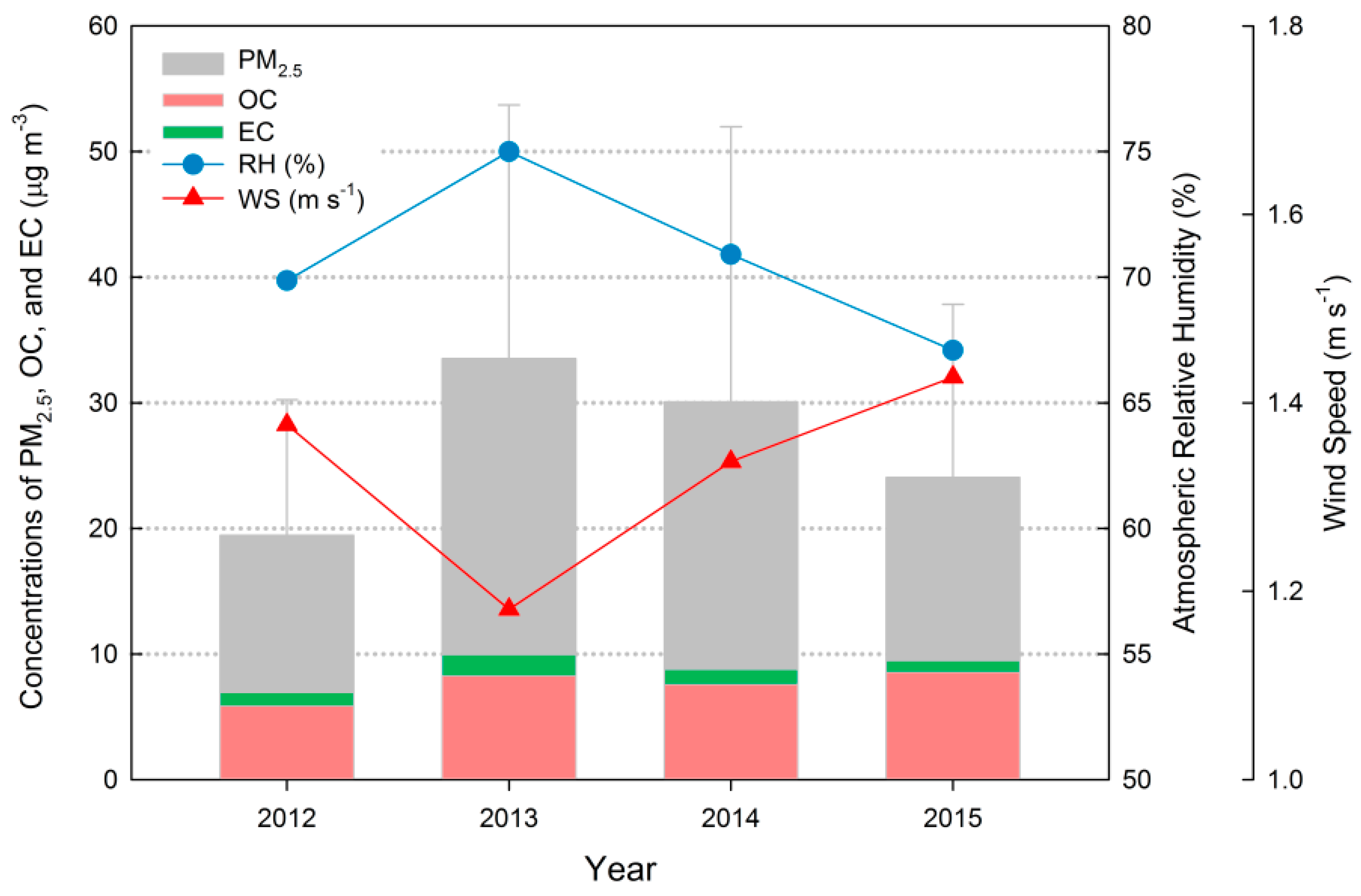
3.1. General Trends
3.2. Primary Organic Carbon (POC) and Secondary Organic Carbon (SOC)
3.3. Water-Soluble Organic Carbon
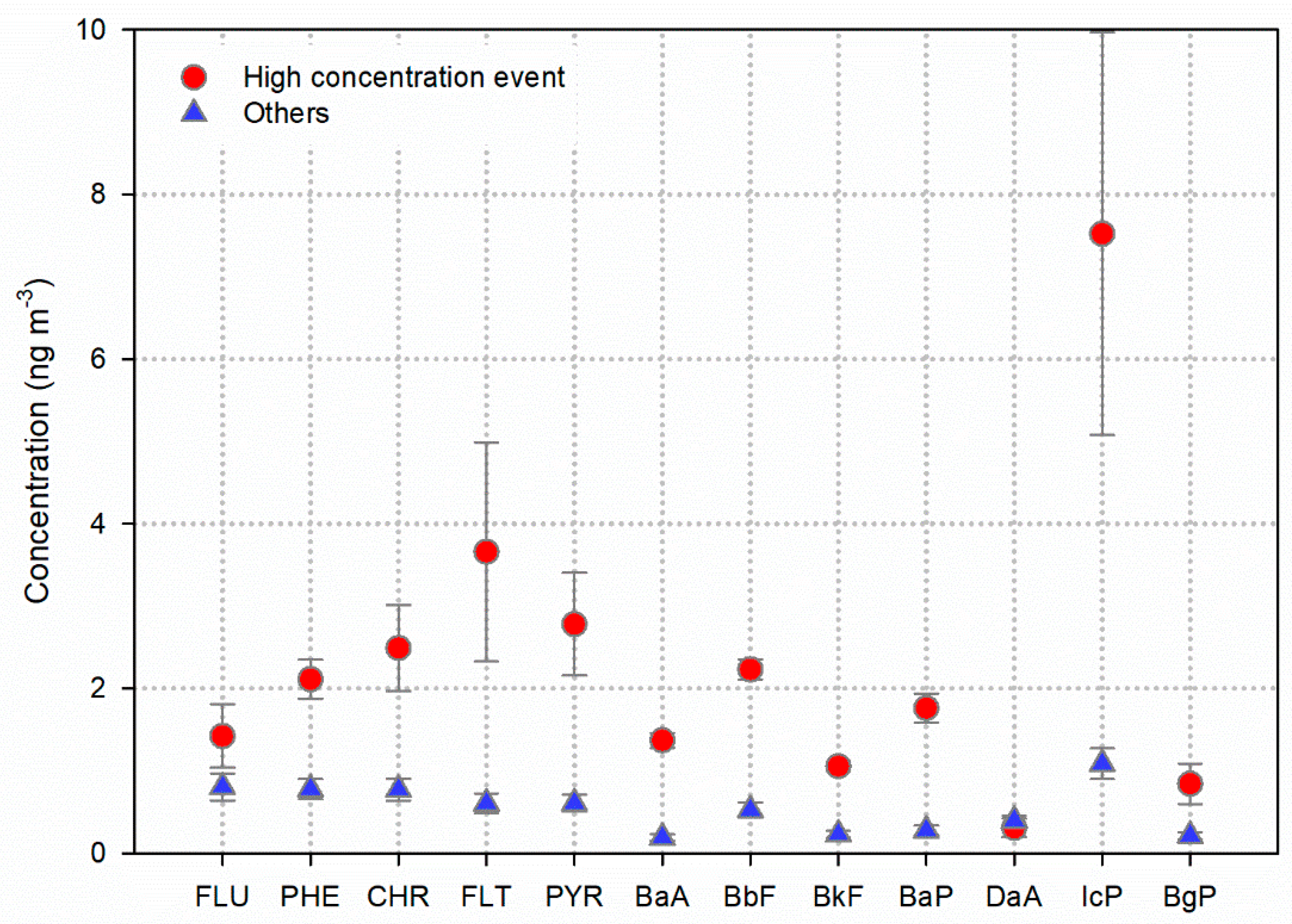
3.4. Polycyclic Aromatic Hydrocarbons
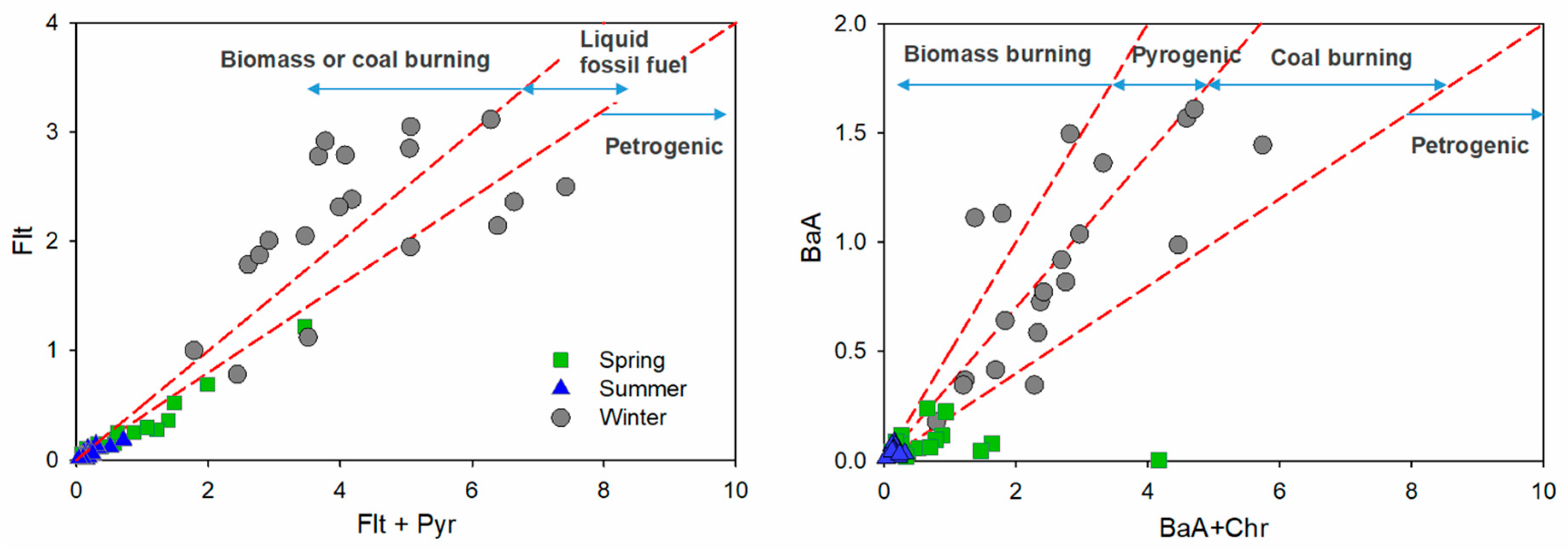
4. Source Identification
5. Conclusions
Supplementary Materials
Author Contributions
Funding
Conflicts of Interest
References
- Joint, W.; World Health Organization. Health Risks of Particulate Matter from Long-Range Transboundary Air Pollution; WHO Regional Office for Europe: Copenhagen, Denmark, 2006. [Google Scholar]
- Grivas, G.; Cheristanidis, S.; Chaloulakou, A. Elemental and organic carbon in the urban environment of Athens. Seasonal and diurnal variations and estimates of secondary organic carbon. Sci. Total Environ. 2012, 414, 535–545. [Google Scholar] [CrossRef] [PubMed]
- Kondo, Y.; Miyazaki, Y.; Takegawa, N.; Miyakawa, T.; Weber, R.; Jimenez, J.L.; Zhang, Q.; Worsnop, D. Oxygenated and water-soluble organic aerosols in Tokyo. J. Geophys. Res. Atmos. 2007, 112. [Google Scholar] [CrossRef]
- Miyazaki, Y.; Kondo, Y.; Takegawa, N.; Komazaki, Y.; Fukuda, M.; Kawamura, K.; Mochida, M.; Okuzawa, K.; Weber, R.J. Time-resolved measurements of water-soluble organic carbon in Tokyo. J. Geophys. Res. Atmos. 2006, 111. [Google Scholar] [CrossRef]
- Sullivan, A.P.; Weber, R.J. Chemical characterization of the ambient organic aerosol soluble in water: 2. Isolation of acid, neutral, and basic fractions by modified size-exclusion chromatography. J. Geophys. Res. Atmos. 2006, 111. [Google Scholar] [CrossRef]
- Yan, B.; Zheng, M.; Hu, Y.; Ding, X.; Sullivan, A.P.; Weber, R.J.; Baek, J.; Edgerton, E.S.; Russell, A.G. Roadside, urban, and rural comparison of primary and secondary organic molecular markers in ambient PM2.5. Environ. Sci. Technol. 2009, 43, 4287–4293. [Google Scholar] [CrossRef]
- Weber, R.J.; Sullivan, A.P.; Peltier, R.E.; Russell, A.; Yan, B.; Zheng, M.; De Gouw, J.; Warneke, C.; Brock, C.; Holloway, J.S. A study of secondary organic aerosol formation in the anthropogenic-influenced southeastern United States. J. Geophys. Res. Atmos. 2007, 112. [Google Scholar] [CrossRef]
- Hecobian, A.; Zhang, X.; Zheng, M.; Frank, N.; Edgerton, E.S.; Weber, R.J. Water-Soluble Organic Aerosol material and the light-absorption characteristics of aqueous extracts measured over the Southeastern United States. Atmos. Chem. Phys. 2010, 10, 5965–5977. [Google Scholar] [CrossRef]
- Pathak, R.K.; Wang, T.; Ho, K.; Lee, S. Characteristics of summertime PM2.5 organic and elemental carbon in four major Chinese cities: Implications of high acidity for water-soluble organic carbon (WSOC). Atmos. Environ. 2011, 45, 318–325. [Google Scholar] [CrossRef]
- Afroz, R.; Hassan, M.N.; Ibrahim, N.A. Review of air pollution and health impacts in Malaysia. Environ. Res. 2003, 92, 71–77. [Google Scholar] [CrossRef]
- Fang, G.; Huang, J.; Huang, Y. Polycyclic Aromatic Hydrocarbon Pollutants in the Asian Atmosphere During 2001 to 2009. Environ. Forensics 2010, 11, 207–215. [Google Scholar] [CrossRef]
- International Agency for Research on Cancer (IARC). Agents Classified by the IARC Monographs; International Agency for Research on Cancer, World Health Organization: Lyon, France, 6937; Volumes 1–109. [Google Scholar]
- Cheng, Z.; Luo, L.; Wang, S.; Wang, Y.; Sharma, S.; Shimadera, H.; Wang, X.; Bressi, M.; de Miranda, R.M.; Jiang, J. Status and characteristics of ambient PM2.5 pollution in global megacities. Environ. Int. 2016, 89, 212–221. [Google Scholar] [CrossRef] [PubMed]
- Han, Y.; Kim, H.; Cho, S.; Kim, P.; Kim, W. Metallic elements in PM2.5 in different functional areas of Korea: Concentrations and source identification. Atmos. Res. 2015, 153, 416–428. [Google Scholar] [CrossRef]
- Vellingiri, K.; Kim, K.; Ma, C.; Kang, C.; Lee, J.; Kim, I.; Brown, R.J. Ambient particulate matter in a central urban area of Seoul, Korea. Chemosphere 2015, 119, 812–819. [Google Scholar] [CrossRef] [PubMed]
- Jeong, J.I.; Park, R.J.; Woo, J.; Han, Y.; Yi, S. Source contributions to carbonaceous aerosol concentrations in Korea. Atmos. Environ. 2011, 45, 1116–1125. [Google Scholar] [CrossRef]
- Matter, P. Speciation Guidance (Final Draft); US Environmental Protection Agency: Research Triangle Park, NC, USA, 1999.
- Birch, M.E.; Cary, R.A. Elemental Carbon-Based Method for Monitoring Occupational Exposures to Particulate Diesel Exhaust. Aerosol Sci. Technol. 1996, 25, 221–241. [Google Scholar] [CrossRef]
- Health Division of Physical Sciences NIOSH. Manual of Analytical Methods; US Department of Health and Human Services, Public Health Service, Centers for Disease Control and Prevention, National Institute for Occupational Safety and Health, Division of Physical Sciences and Engineering: Atlanta, GA, USA, 1994.
- US EPA. Method 8100 Polynuclear Aromatic Hydrocarbons; US EPA: Washington, DC, USA, 1986; pp. 1–10.
- Ott, W.R. Environmental Statistics and data Analysis; CRC Press: Boca Raton, FL, USA, 1995. [Google Scholar]
- Hu, D.; Jiang, J. PM2.5 pollution and risk for lung cancer: A rising issue in China. J. Environ. Prot. 2014, 5, 731. [Google Scholar] [CrossRef]
- Kamens, R.M.; Zhang, H.; Chen, E.H.; Zhou, Y.; Parikh, H.M.; Wilson, R.L.; Galloway, K.E.; Rosen, E.P. Secondary organic aerosol formation from toluene in an atmospheric hydrocarbon mixture: Water and particle seed effects. Atmos. Environ. 2011, 45, 2324–2334. [Google Scholar] [CrossRef]
- Jung, J.-H.; Han, Y.-J. Study on Characteristics of PM2.5 and Its Ionic Constituents in Chuncheon, Korea. J. Korean Soc. Atmos. Environ. 2008, 24, 682–692. [Google Scholar] [CrossRef]
- Kozáková, J.; Pokorná, P.; Černíková, A.; Hovorka, J.; Braniš, M.; Moravec, P.; Schwarz, J. The association between intermodal (PM1–2.5) and PM1, PM2.5, coarse fraction and meteorological parameters in various environments in Central Europe. Aerosol Air Qual. Res. 2017, 17, 1234–1243. [Google Scholar] [CrossRef]
- Kozáková, J.; Leoni, C.; Klán, M.; Hovorka, J.; Racek, M.; Koštejn, M.; Ondráček, J.; Moravec, P.; Schwarz, J. Chemical Characterization of PM1–2.5 and its Associations with PM1, PM2.5–10 and Meteorology in Urban and Suburban Environments. Aerosol Air Qual. Res. 2018, 18, 1684–1697. [Google Scholar] [CrossRef]
- Jeon, H.; Park, J.; Kim, H.; Sung, M.; Choi, J.; Hong, Y.; Hong, J. The characteristics of PM2.5 concentration and chemical composition of Seoul metropolitan and inflow background area in Korea peninsula. J. Korean Soc. Urban Environ. 2015, 15, 261–271. [Google Scholar]
- Choi, J.; Heo, J.; Ban, S.; Yi, S.; Zoh, K. Chemical characteristics of PM2.5 aerosol in Incheon, Korea. Atmos. Environ. 2012, 60, 583–592. [Google Scholar] [CrossRef]
- Park, S.S.; Cho, S.Y.; Kim, S.J. Chemical Characteristics of Water Soluble Components in Fine Particulate Matter at a Gwangju area. Korean Chem. Eng. Res. 2010, 48, 20–26. [Google Scholar]
- Han, J.; Kim, J.; Kang, E.; Lee, M.; Shim, J. Ionic Compositions and Carbonaceous Matter of PM2.5 at Ieodo Ocean Research Station. J. Korean Soc. Atmos. Environ. 2013, 29, 701–712. [Google Scholar] [CrossRef]
- Kim, H.; Jung, J.; Lee, J.; Lee, S. Seasonal Characteristics of Organic Carbon and Elemental Carbon in PM2.5 in Daejeon. J. Korean Soc. Atmos. Environ. 2015, 31, 28–40. [Google Scholar] [CrossRef]
- Kang, B.W.; Lee, H.S. Source Apportionment of Fine Particulate Matter (PM2.5) in the Chungju City. J. Korean Soc. Atmos. Environ. 2015, 31, 437–448. [Google Scholar] [CrossRef]
- Li, K.C.; Hwang, I. Characteristics of PM2.5 in Gyeongsan Using Statistical Analysis. J. Korean Soc. Atmos. Environ. 2015, 31, 520–529. [Google Scholar] [CrossRef]
- Paraskevopoulou, D.; Liakakou, E.; Gerasopoulos, E.; Theodosi, C.; Mihalopoulos, N. Long-term characterization of organic and elemental carbon in the PM2.5 fraction: The case of Athens, Greece. Atmos. Chem. Phys. 2014, 14, 13313–13325. [Google Scholar] [CrossRef]
- Plaza, J.; Artíñano, B.; Salvador, P.; Gómez-Moreno, F.J.; Pujadas, M.; Pio, C.A. Short-term secondary organic carbon estimations with a modified OC/EC primary ratio method at a suburban site in Madrid (Spain). Atmos. Environ. 2011, 45, 2496–2506. [Google Scholar] [CrossRef]
- Zhang, R.; Tao, J.; Ho, K.; Shen, Z.; Wang, G.; Cao, J.; Liu, S.; Zhang, L.; Lee, S. Characterization of atmospheric organic and elemental carbon of PM2.5 in a typical semi-arid area of Northeastern China. Aerosol Air Qual. Res. 2012, 12, 792–802. [Google Scholar] [CrossRef]
- Schauer, J.J.; Kleeman, M.J.; Cass, G.R.; Simoneit, B.R. Measurement of emissions from air pollution sources. 2. C1 through C30 organic compounds from medium duty diesel trucks. Environ. Sci. Technol. 1999, 33, 1578–1587. [Google Scholar] [CrossRef]
- Schauer, J.J.; Kleeman, M.J.; Cass, G.R.; Simoneit, B.R. Measurement of emissions from air pollution sources. 5. C1−C32 organic compounds from gasoline-powered motor vehicles. Environ. Sci. Technol. 2002, 36, 1169–1180. [Google Scholar] [CrossRef] [PubMed]
- Chen, Y.; Zhi, G.; Feng, Y.; Fu, J.; Feng, J.; Sheng, G.; Simoneit, B.R. Measurements of emission factors for primary carbonaceous particles from residential raw-coal combustion in China. Geophys. Res. Lett. 2006, 33. [Google Scholar] [CrossRef]
- Schauer, J.J.; Kleeman, M.J.; Cass, G.R.; Simoneit, B.R. Measurement of emissions from air pollution sources. 3. C1−C29 organic compounds from fireplace combustion of wood. Environ. Sci. Technol. 2001, 35, 1716–1728. [Google Scholar] [CrossRef] [PubMed]
- He, L.; Hu, M.; Huang, X.; Yu, B.; Zhang, Y.; Liu, D. Measurement of emissions of fine particulate organic matter from Chinese cooking. Atmos. Environ. 2004, 38, 6557–6564. [Google Scholar] [CrossRef]
- Gu, J.; Bai, Z.; Liu, A.; Wu, L.; Xie, Y.; Li, W.; Dong, H.; Zhang, X. Characterization of atmospheric organic carbon and element carbon of PM2.5 and PM10 at Tianjin, China. Aerosol Air Qual. Res. 2010, 10, 167–176. [Google Scholar] [CrossRef]
- Chow, J.C.; Watson, J.G.; Kuhns, H.; Etyemezian, V.; Lowenthal, D.H.; Crow, D.; Kohl, S.D.; Engelbrecht, J.P.; Green, M.C. Source profiles for industrial, mobile, and area sources in the Big Bend Regional Aerosol Visibility and Observational study. Chemosphere 2004, 54, 185–208. [Google Scholar] [CrossRef] [PubMed]
- Grabowsky, J.; Streibel, T.; Sklorz, M.; Chow, J.C.; Watson, J.G.; Mamakos, A.; Zimmermann, R. Hyphenation of a carbon analyzer to photo-ionization mass spectrometry to unravel the organic composition of particulate matter on a molecular level. Anal. Bioanal. Chem. 2011, 401, 3153–3164. [Google Scholar] [CrossRef]
- Cao, J.; Huang, H.; Lee, S.; Chow, J.C.; Zou, C.; Ho, K.; Watson, J.G. Indoor/outdoor relationships for organic and elemental carbon in PM2.5 at residential homes in Guangzhou, China. Aerosol Air Qual. Res. 2012, 12, 902–910. [Google Scholar] [CrossRef]
- Turpin, B.J.; Huntzicker, J.J. Identification of secondary organic aerosol episodes and quantitation of primary and secondary organic aerosol concentrations during SCAQS. Atmos. Environ. 1995, 29, 3527–3544. [Google Scholar] [CrossRef]
- Chu, S. Stable estimate of primary OC/EC ratios in the EC tracer method. Atmos. Environ. 2005, 39, 1383–1392. [Google Scholar] [CrossRef]
- Saylor, R.D.; Edgerton, E.S.; Hartsell, B.E. Linear regression techniques for use in the EC tracer method of secondary organic aerosol estimation. Atmos. Environ. 2006, 40, 7546–7556. [Google Scholar] [CrossRef]
- Na, K.; Sawant, A.; Song, C.; Cocker, D., III. Primary and secondary carbonaceous species in the atmosphere of Western Riverside County, California. Atmos. Environ. 2004, 38, 1345–1355. [Google Scholar]
- Claeys, M.; Graham, B.; Vas, G.; Wang, W.; Vermeylen, R.; Pashynska, V.; Cafmeyer, J.; Guyon, P.; Andreae, M.O.; Artaxo, P.; et al. Formation of secondary organic aerosols through photooxidation of isoprene. Science 2004, 303, 1173–1176. [Google Scholar] [CrossRef]
- Schichtel, B.A.; Malm, W.C.; Bench, G.; Fallon, S.; McDade, C.E.; Chow, J.C.; Watson, J.G. Fossil and contemporary fine particulate carbon fractions at 12 rural and urban sites in the United States. J. Geophys. Res. Atmos. 2008, 113. [Google Scholar] [CrossRef]
- Wu, D.; Wang, Z.; Chen, J.; Kong, S.; Fu, X.; Deng, H.; Shao, G.; Wu, G. Polycyclic aromatic hydrocarbons (PAHs) in atmospheric PM2.5 and PM10 at a coal-based industrial city: Implication for PAH control at industrial agglomeration regions, China. Atmos. Res. 2014, 149, 217–229. [Google Scholar] [CrossRef]
- Kong, S.; Ding, X.; Bai, Z.; Han, B.; Chen, L.; Shi, J.; Li, Z. A seasonal study of polycyclic aromatic hydrocarbons (PAHs) in PM2.5 and PM2.5-10 in five typical cities of Liaoning Province, China. J. Hazard. Mater. 2010, 183, 70–80. [Google Scholar] [CrossRef] [PubMed]
- Lee, J.Y.; Kim, Y.P.; Kang, C.; Ghim, Y.S.; Kaneyasu, N. Temporal trend and long-range transport of particulate polycyclic aromatic hydrocarbons at Gosan in northeast Asia between 2001 and 2004. J. Geophys. Res. Atmos. 2006, 111. [Google Scholar] [CrossRef]
- Liu, Y.; Yu, Y.; Liu, M.; Lu, M.; Ge, R.; Li, S.; Liu, X.; Dong, W.; Qadeer, A. Characterization and source identification of PM2.5-bound polycyclic aromatic hydrocarbons (PAHs) in different seasons from Shanghai, China. Sci. Total Environ. 2018, 644, 725–735. [Google Scholar] [CrossRef]
- Dachs, J.; Glenn IV, T.R.; Gigliotti, C.L.; Brunciak, P.; Totten, L.A.; Nelson, E.D.; Franz, T.P.; Eisenreich, S.J. Processes driving the short-term variability of polycyclic aromatic hydrocarbons in the Baltimore and northern Chesapeake Bay atmosphere, USA. Atmos. Environ. 2002, 36, 2281–2295. [Google Scholar] [CrossRef]
- Khan, M.F.; Latif, M.T.; Lim, C.H.; Amil, N.; Jaafar, S.A.; Dominick, D.; Nadzir, M.S.M.; Sahani, M.; Tahir, N.M. Seasonal effect and source apportionment of polycyclic aromatic hydrocarbons in PM2.5. Atmos. Environ. 2015, 106, 178–190. [Google Scholar] [CrossRef]
- Yunker, M.B.; Macdonald, R.W.; Vingarzan, R.; Mitchell, R.H.; Goyette, D.; Sylvestre, S. PAHs in the Fraser River basin: A critical appraisal of PAH ratios as indicators of PAH source and composition. Org. Geochem. 2002, 33, 489–515. [Google Scholar] [CrossRef]
- Roberto, J.; Lee, W.; Campos-Díaz, S.I. Soil-borne polycyclic aromatic hydrocarbons in El Paso, Texas: Analysis of a potential problem in the United States/Mexico border region. J. Hazard. Mater. 2009, 163, 946–958. [Google Scholar]


| Gas | Hold Time (s) | Temperature (°C) | Component |
|---|---|---|---|
| He | 10 | 1 | |
| He | 80 | 310 | OC1 |
| He | 80 | 475 | OC2 |
| He | 80 | 615 | OC3 |
| He | 110 | 870 | OC4 |
| He | 45 | 550 | PC |
| O2 in He | 45 | 550 | EC1 |
| O2 in He | 45 | 625 | EC2 |
| O2 in He | 45 | 700 | EC3 |
| O2 in He | 45 | 775 | EC4 |
| O2 in He | 45 | 850 | EC5 |
| O2 in He | 110 | 870 | EC6 |
| Compounds | R2 | MDL (ng) | RSD (%) | Recovery (%) | Detector |
|---|---|---|---|---|---|
| FLU | 0.9985 | 0.14 | 1.9 | 78.2 | UV |
| PHE | 0.9979 | 0.11 | 6.7 | 65.9 | UV |
| CHR | 0.9994 | 0.17 | 2.9 | 76.4 | UV |
| FLT | 0.9995 | 0.08 | 1.5 | 91.8 | FLD |
| PYR | 0.9987 | 0.01 | 1.4 | 135.9 | FLD |
| BaA | 0.9990 | 0.01 | 1.1 | 109.7 | FLD |
| BbF | 0.9989 | 0.02 | 1.0 | 99.9 | FLD |
| BkF | 0.9985 | 0.01 | 0.1 | 92.3 | FLD |
| BaP | 0.9983 | 0.04 | 1.0 | 110.2 | FLD |
| DaA | 0.9991 | 0.03 | 1.2 | 106.7 | FLD |
| IcP | 0.9944 | 0.01 | 2.3 | 120.5 | FLD |
| BgP | 0.9930 | 0.00 | 2.5 | 131.5 | FLD |
| Period | N | PM2.5 | OC | EC | |
|---|---|---|---|---|---|
| POC | SOC | ||||
| Spring | 98 | 29.1 ± 17.5 | 4.9 ± 2.4 (64%) | 2.8 ± 1.9 (36%) | 1.1 ± 0.5 (3.9) |
| Summer | 103 | 16.9 ± 11.1 | 2.9 ± 1.3 (49%) | 3.0 ± 2.7 (51%) | 0.7 ± 0.3 (3.9) |
| Autumn | 65 | 24.5 ± 12.7 | 4.4 ± 3.3 (61%) | 2.8 ± 2.3 (39%) | 1.3 ± 1.0 (5.5) |
| Winter | 97 | 40.5 ± 22.1 | 6.1 ± 4.1 (56%) | 4.7 ± 3.3 (44%) | 1.8 ± 1.3 (4.5) |
| Total | 363 | 27.8 ± 18.8 | 4.7 ± 3.3 (58%) | 3.4 ± 2.7 (42%) | 1.2 ± 0.9 (4.4) |
| Site | Site Type | Period | PM2.5 | OC | EC | OC/EC | References |
|---|---|---|---|---|---|---|---|
| Seoul, Korea | Urban | January 2013~December 2013 | 29.5 | 4.8 | 1.8 | 2.7 | [27] |
| Incheon, Korea | Industrial | January 2009~May 2010 | 41.9 | 7.9 | 1.8 | 4.4 | [28] |
| Gwangju, Korea | Urban | December 2007~February 2008 | 27.4 | 4.5 | 1.8 | 2.7 | [29] |
| Ieodo, Korea | Rural | June 2006~June 2008 | 21.8 | 2.3 | 1.0 | 2.3 | [30] |
| Daejeon, Korea | Urban | March 2012~February 2013 | 23.6 | 5.3 | 0.8 | 6.6 | [31] |
| Chungju, Korea | Suburban | May 2013~January 2014 | 48.2 | 5.8 | 1.8 | 3.2 | [32] |
| Gyeongsan, Korea | Suburban | September 2010~December 2012 | 25.2 | 4.3 | 1.3 | 3.3 | [33] |
| Chuncheon | Suburban | April 2012~August 2015 | 27.8 | 7.8 | 1.2 | 7.7 | This study |
| Beijing, China | Urban | June~August 2005 | 68.0 | 8.2 | 4.9 | 2.2 | [9] |
| Athens, Greece | Urban | May 2008~April 2013 | 20.0 | 2.0 | 0.5 | 4.7 | [34] |
| Madrid, Spain | Urban | February 2006~June 2008 | - | 3.7 | 1.3 | 4.3 | [35] |
| Tongyu, China | Rural | April~June 2006 | - | 14.1 | 2.0 | 7.5 | [36] |
| Season | N | Deming Regression Derived (y = bx + a) |
|---|---|---|
| Spring | 11 | y = 4.3x + 0.07 |
| Summer | 7 | y = 4.7x |
| Fall | 6 | y = 3.2x + 0.11 |
| Winter | 12 | y = 3.5x + 0.02 |
| Species | No. of Rings | Winter | Spring | Summer |
|---|---|---|---|---|
| PM2.5 (μg m−3) | 37.3 ± 14.7 | 23.0 ± 17.1 | 13.2 ± 8.1 | |
| 12 PAHs (ng m−3) | ||||
| FLU | 3 | 1.4 ± 1.0 | 0.2 ± 0.0 | 0.4 ± 0.3 |
| PHE | 3 | 1.6 ± 0.7 | 0.5 ± 0.4 | 0.3 ± 0.3 |
| CHR | 4 | 1.8 ± 1.0 | 0.8 ± 1.0 | 0.1 ± 0.1 |
| FLT | 4 | 2.7 ± 2.2 | 0.4 ± 0.4 | 0.1 ± 0.0 |
| PYR | 4 | 2.1 ± 1.3 | 0.6 ± 0.6 | 0.1 ± 0.1 |
| BaA | 4 | 0.9 ± 0.5 | 0.1 ± 0.1 | - |
| BbF | 5 | 1.9 ± 0.6 | 0.4 ± 0.4 | 0.1 ± 0.1 |
| BkF | 5 | 0.9 ± 0.3 | 0.2 ± 0.2 | - |
| BaP | 5 | 1.3 ± 0.6 | 0.2 ± 0.2 | 0.1 ± 0.0 |
| DaA | 5 | 0.3 ± 0.3 | 0.2 ± 0.2 | 0.6 ± 0.5 |
| IcP | 6 | 4.2 ± 4.9 | 1.8 ± 1.9 | 0.3 ± 0.3 |
| BgP | 6 | 0.8 ± 0.5 | 0.2 ± 0.2 | - |
| ∑PAHs | 19.8 ± 8.1 | 5.4 ± 3.6 | 2.1 ± 0.8 | |
| LMW PAHs | 3 | 3.0 ± 1.3 (15.2%) | 0.7 ± 0.3 (13.0%) | 0.6 ± 0.4 (28.6%) |
| MMW PAHs | 4 | 7.4 ± 3.0 (37.4%) | 1.9 ± 1.3 (35.2%) | 0.3 ± 0.2 (14.3%) |
| HMW PAHs | 5,6 | 9.3 ± 5.2 (47.0%) | 2.8 ± 2.6 (51.9%) | 1.1 ± 0.5 (52.4%) |
© 2018 by the authors. Licensee MDPI, Basel, Switzerland. This article is an open access article distributed under the terms and conditions of the Creative Commons Attribution (CC BY) license (http://creativecommons.org/licenses/by/4.0/).
Share and Cite
Park, J.-M.; Han, Y.-J.; Cho, S.-H.; Kim, H.-W. Characteristics of Carbonaceous PM2.5 in a Small Residential City in Korea. Atmosphere 2018, 9, 490. https://doi.org/10.3390/atmos9120490
Park J-M, Han Y-J, Cho S-H, Kim H-W. Characteristics of Carbonaceous PM2.5 in a Small Residential City in Korea. Atmosphere. 2018; 9(12):490. https://doi.org/10.3390/atmos9120490
Chicago/Turabian StylePark, Jong-Min, Young-Ji Han, Sung-Hwan Cho, and Hyun-Woong Kim. 2018. "Characteristics of Carbonaceous PM2.5 in a Small Residential City in Korea" Atmosphere 9, no. 12: 490. https://doi.org/10.3390/atmos9120490
APA StylePark, J.-M., Han, Y.-J., Cho, S.-H., & Kim, H.-W. (2018). Characteristics of Carbonaceous PM2.5 in a Small Residential City in Korea. Atmosphere, 9(12), 490. https://doi.org/10.3390/atmos9120490