Comparison of Simulated Tropical Cyclone Intensity and Structures Using the WRF with Hydrostatic and Nonhydrostatic Dynamical Cores

Abstract

This study explored the influence of choosing a nonhydrostatic dynamical core or a hydrostatic dynamical core in the weather research and forecasting (WRF) model on the intensity and structure of simulated tropical cyclones (TCs). A comparison of cloud-resolving simulations using each core revealed significant differences in the TC simulations. In comparison with the nonhydrostatic simulation, the hydrostatic simulation produced a stronger and larger TC, associated with stronger convective activity. A budget analysis of the vertical momentum equation was conducted to investigate the underlying mechanisms. Although the hydrostatic dynamical core was used, the vertical motion was not in strict hydrostatic balance because of the existence of the vertical perturbation pressure gradient force, local buoyancy force, water loading, and sum of the Coriolis and diffusion effects. The contribution of the enhanced vertical perturbation pressure gradient force was found to be more important for stronger upward acceleration in the eyewall in the hydrostatic simulation than in the nonhydrostatic simulation. This is because it leads to intensified convection in the eyewall that releases more latent heat, which induces a larger low-level radial pressure gradient and inflow motion, and eventually leads to a stronger storm.

1. Introduction

The hydrostatic approximation, which assumes a local balance between the gravitational and vertical pressure gradient forces, was established initially based on scale analysis [1,2]. It has been validated for meso-α, synoptic, and global-scale circulations, and thus it could be considered a reliable and accurate assumption [3]. As one of the fundamental assumptions adopted in atmospheric and oceanic models [3,4,5], the hydrostatic approximation has been incorporated in numerical weather prediction models for decades to allow longer time steps by filtering out vertically propagating sound waves [6].

Following the rapid improvement of computing resources in recent years, the use of nonhydrostatic numerical models has become widespread. With the aid of new numerical treatments designed to handle sound waves, e.g., semi-implicit [7] and split-explicit techniques [8], nonhydrostatic mesoscale models have developed rapidly, and they have been used actively in research and operational communities during the previous two decades [6]. However, global climate models remain mostly based on hydrostatic atmospheric dynamical cores, even though the increase in computational cost associated with the use of a nonhydrostatic dynamical core is not particularly large [9].

Previous studies have used different methods to compare the discrepancies between hydrostatic and nonhydrostatic models in simulating weather phenomena. Based on analytical solutions, the characteristics of hydrostatic and nonhydrostatic flows have been studied theoretically [10,11]. Furthermore, idealized experiments have been conducted to validate nonhydrostatic mesoscale models in situations that include mountain waves over a bell-shaped mountain, density currents produced by a cold bubble, and rising thermal bubble cases [6,12,13]. These previous studies found that two-dimensional idealized cases were reproduced well only in nonhydrostatic experiments.

As might be expected, real-case simulations demonstrated that nonhydrostatic mesoscale models are superior to hydrostatic models in high-resolution precipitation forecasts [14,15,16,17]. However, it should be noted that such simulations were conducted with a grid spacing smaller than 10 km, which is traditionally considered the hydrostatic limit in the absence of latent heat release [18]. Meanwhile, Dudhia [19] identified a “gray zone” of the dynamics and it remains unclear whether nonhydrostatic dynamics should be applied within this zone. He suggested the scale of the gray zone depends on the scale of the weather characteristics and that it would be within the range of a grid size of <5 km. In addition, Dudhia [14] found that nonhydrostatic effects start to appear in a simulation of a cold front when the horizontal grid spacing is <5 km. A hydrostatic simulation with a 5-km grid spacing tends to overestimate and over-enlarge the area of precipitation [15] Also, hydrostatic mesoscale models do not perform as well as nonhydrostatic models in the prediction of synoptic fields and precipitation forecasts with a 10-km grid spacing [17].

Nonhydrostatic effects in hurricanes are conventionally considered small for large-scale systems. However, for tropical cyclones, vertical motion plays a crucial role in the inner-core region, and hence the nonhydrostatic impacts could be important. Besides this, the vertical motion in the eyewall of TCs is weaker than in other severe storms such as tornadoes and mid-latitude thunderstorms [20] Zhang et al. [21] suggested that hydrostatic models might be used to simulate hurricanes using a grid size of <6 km, providing that some cloud microphysics processes and water loading were incorporated properly. Although several studies have compared the effects of using both hydrostatic and nonhydrostatic dynamical cores in simulations of severe weather phenomena [6,9], an examination of the influence of both cores in simulations of tropical cyclone (TC) intensity and structure, especially at high resolution, is still lacking. The objective of this study was to examine the differences between hydrostatic and nonhydrostatic simulations of TC intensity and structure using the weather research and forecasting [22] model as a tool at cloud-resolving resolutions. The remainder of this paper is organized as follows. Section 2 describes the model configuration and numerical experiments. The derived results are discussed in Section 3. Finally, a summary and a discussion are presented in Section 4.

2. Model Setup and Experimental Design

The WRF model was set on an $f$ plane at 20° N, configured with three domains with horizontal resolutions of 15, 5, and 1.67 km and dimensions of 220 × 220, 202 × 202, and 301 × 301, respectively. The nested domains moved automatically to follow the TC center. There were 31 levels placed as default in the vertical direction, with the model top set at 50 hPa. The microphysical processes were modeled by the Lin scheme [23]. The radiation schemes were parameterized by the Dudhia shortwave [24] and rapid radiative transfer model (RRTM) longwave [25] schemes. The boundary layer processes were parameterized using the Yonsei University (YSU) scheme [26]. The surface layer scheme tied to the YSU scheme was the Monin–Obukhov scheme.

For the hydrostatic option, hydrostatic pressure was diagnosed using the definition of the terrain-following hydrostatic pressure vertical coordinate, and the (inverse) density was diagnosed using the equation of state and the proposed potential temperature. Geopotential was diagnosed using the hydrostatic equation, and vertical velocity was diagnosed from the geopotential. For the nonhydrostatic option, the vertical momentum and geopotential equations were used to derive the vertical velocity and geopotential using a linearized state equation [22]. In the nonhydrostatic dynamical solver, the horizontal pressure gradient was calculated by

$$-\frac{\alpha }{{\alpha }_d}[{\mu }_d(\frac{\partial {\mathsf{\Phi }}^{\prime }}{\partial x}+\alpha \frac{\partial p^{\prime }}{\partial x}+{\alpha }_d^{\prime }\frac{\alpha \overline{p}}{\partial x})+\frac{\partial \mathsf{\Phi }}{\partial x}(\frac{\partial p^{\prime }}{\partial \eta }-{\mu }_d^{\prime })]$$

(1)

where $\alpha$, $\mu$, $p$, $\mathsf{\Phi }$, and $\eta$ represent the inverse density, mass per unit area, pressure, geopotential, and hydrostatic pressure coordinate parameter, respectively. Here, subscript “$d$” denotes dry air, the bar above denotes the mean hydrostatic reference state, and the prime denotes the perturbation from the mean reference state [9] In the hydrostatic dynamical solver, because of the hydrostatic balance, the vertical pressure gradient can be expressed as

$$\frac{\partial p^{\prime }}{\partial \eta }=\frac{{\alpha }_d}{\alpha }{\mu }_d-{\overline{\mu }}_d$$

(2)

Combining Equations (1) and (2) means that the horizontal pressure gradient can be simplified as

$${\mu }_d(\frac{\partial {\mathsf{\Phi }}^{\prime }}{\partial x}+\alpha \frac{\partial p^{\prime }}{\partial x}+{{\alpha }^{\prime }}_d\frac{\partial \overline{p}}{\partial x})$$

(3)

To investigate and compare the differences between hydrostatic and nonhydrostatic simulations, two experiments were conducted using the WRF model: one adopting the nonhydrostatic core (denoted CTRL) and the other adopting the hydrostatic core (denoted HY). Both runs were integrated for 120 h with a 30-min output interval.

3. Results

3.1. Intensity and Size Evolution

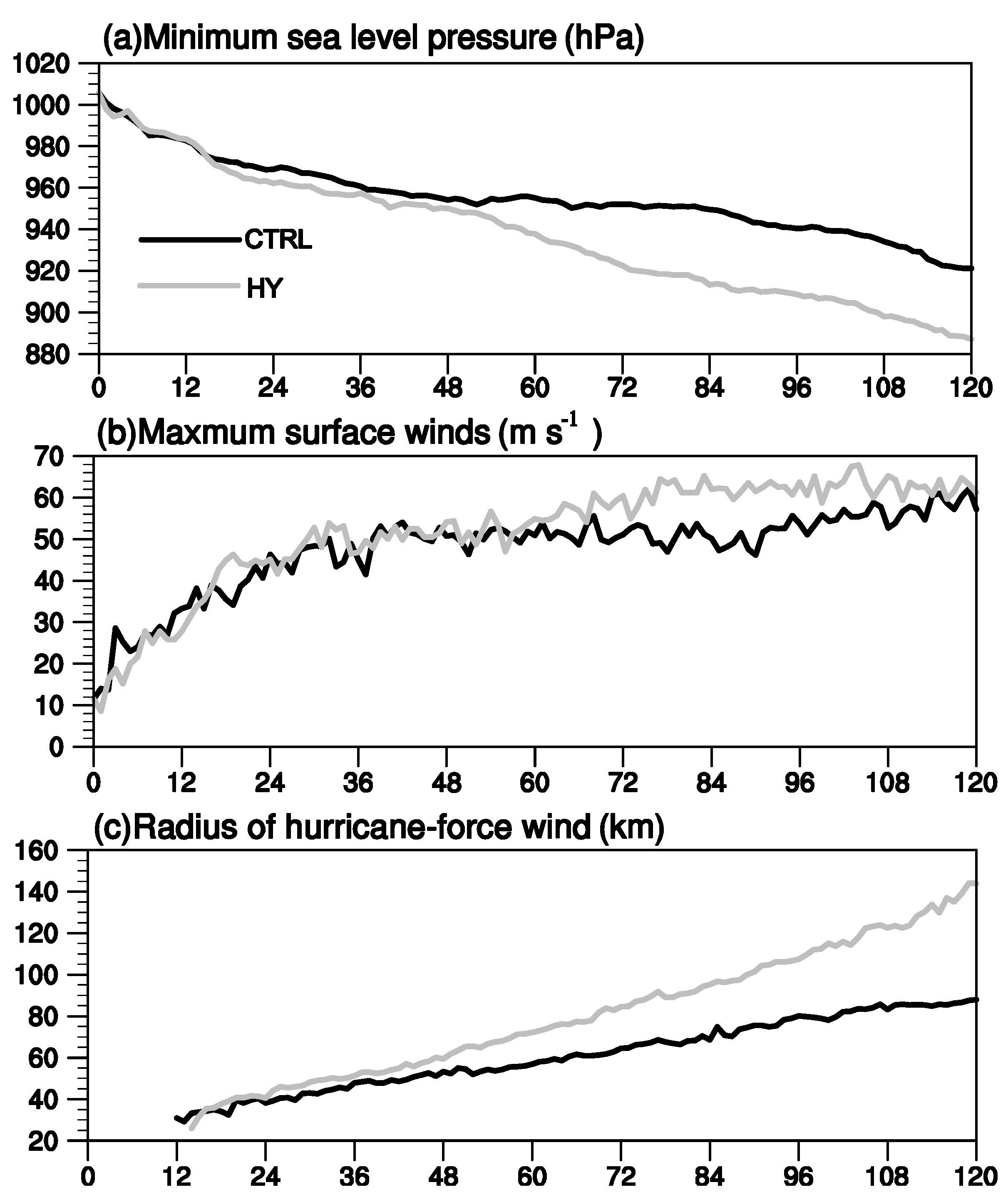
As the storm originated in a quiescent environment on an $f$ plane, it effectively remained stationary during the simulation (not shown). Figure 1 shows the evolution of the storm intensity and size in terms of the minimum sea level pressure, the maximum azimuthal mean wind speed at the lowest model level (about 30 m altitude), and the radius of hurricane-force (33 m s⁻¹) wind for both runs. During the spin-up period, the storm intensifies rapidly and it expands steadily as the moist processes, low-level inflow, and upper-level outflow become progressively established (not shown). During the period from 18 h to 48 h, the difference in intensity between HY and CTRL tends to increase very gradually, i.e., although the storm in HY is stronger than in CTRL, the storm central pressure difference is <10 hPa and the difference in surface wind speed is <10 m s⁻¹. After about 48 h, the rate of intensification gradually slows, attaining a maximum surface wind speed of 55 m s⁻¹ and a minimum sea level pressure of 945 hPa at about 54 h. During the latter stage of the simulations, the TC intensities of the two simulations present substantial differences. After 84 h, both storms continue intensifying and their maximum sea level pressure deviation is as large as 36 hPa by the end of the runs.

Similar to the relationship of intensity, the expansion of storm size in CTRL is faster than in HY. The difference in storm size tends to increase gradually with time. Overall, the TC size in HY is much larger than in CTRL, i.e., by the end of the simulation, the expansion of the storm in HY is approximately 55 km (60%) greater compared with CTRL. The enlarged TC size in the HY simulation is associated primarily with the active outer rainbands. This indicates that the greater release of latent heat by the active rainbands in HY contributes to the larger TC size in HY relative to CTRL In the following sections, to elucidate the impact of nonhydrostatic processes on TC intensity and structure, the period between 84 and 96 h, which produced the greatest differences in TC intensity between the two runs, is considered for further analysis.

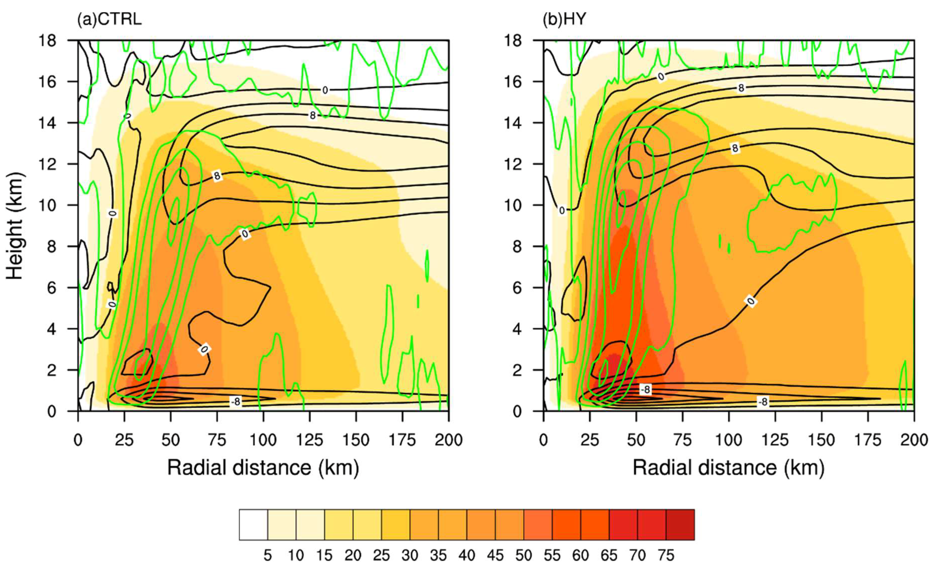
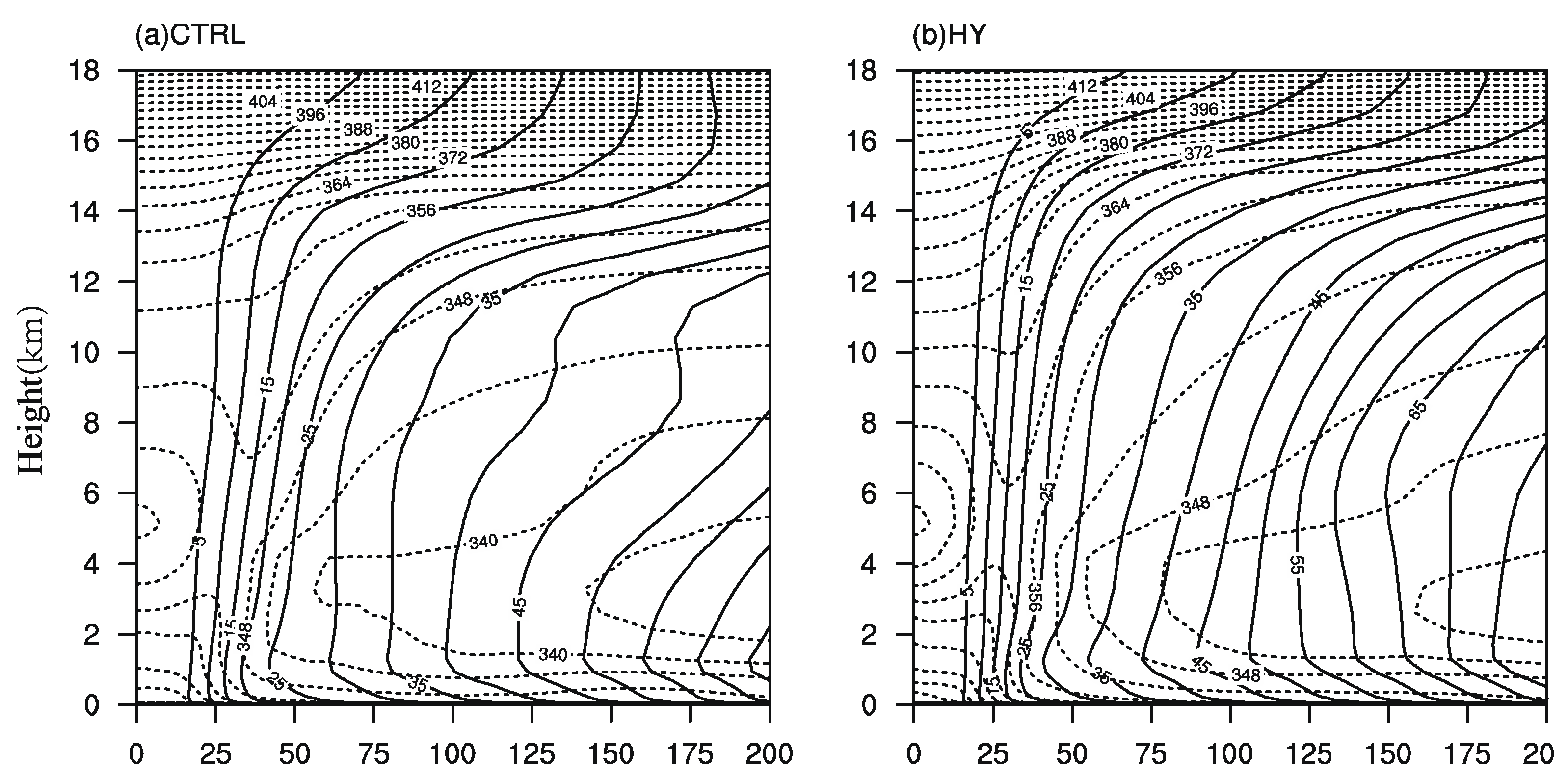
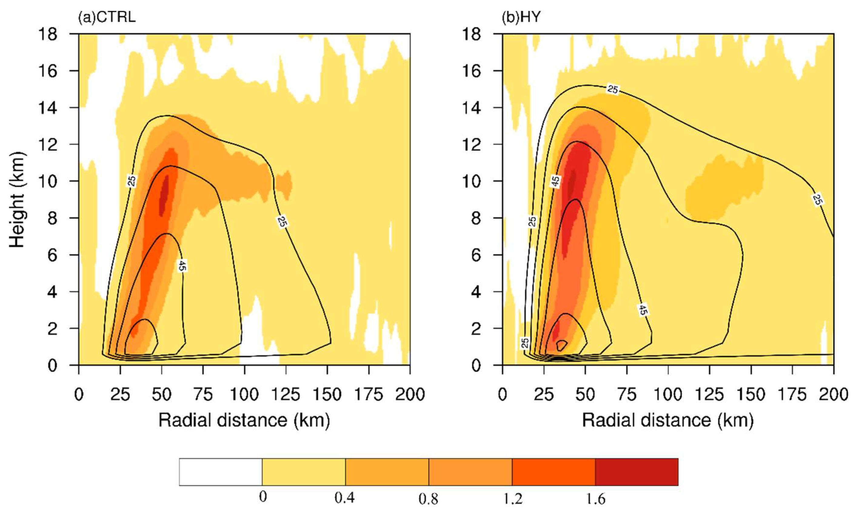
The azimuthal mean winds of CTRL and HY exhibit the typical structures of real TCs (Figure 2), i.e., radial inflow in the boundary layer, radial outflow in the upper troposphere, a secondary outflow jet immediately above the inflow layer, and tangential winds with peak values within the inflow layer [27,28]. Some of the air mass at the top of the TC eyewall returns to the eye and it descends all the way to the lower levels through a narrow zone at the inner edge of the eyewall (Figure 2a). Consistent with the relationship of intensity, the tangential winds are stronger in HY than in CTRL, and the eyewall in CTRL is tilted further outward in comparison with HY, as indicated by the updraft shown in Figure 2. The TC in HY has a stronger and higher upward motion than in CTRL. The sloped vertical motion in CTRL exhibits a “wedge” shape, which is much thinner than in HY below the altitude of about 8 km. The maximum tangential wind appears in the inflow layer of the storm and reaches 75 m s⁻¹ at the radius of 30 km and the altitude of 1 km in HY. Conversely, the maximum tangential wind is only 65 m s⁻¹ in CTRL at the same position. The faster radial inflow in HY is linked to stronger convection in the eyewall. The intensity and structure of the modeled TCs are generally consistent with observations [29], indicating that the following analysis based on the model output data is reliable.

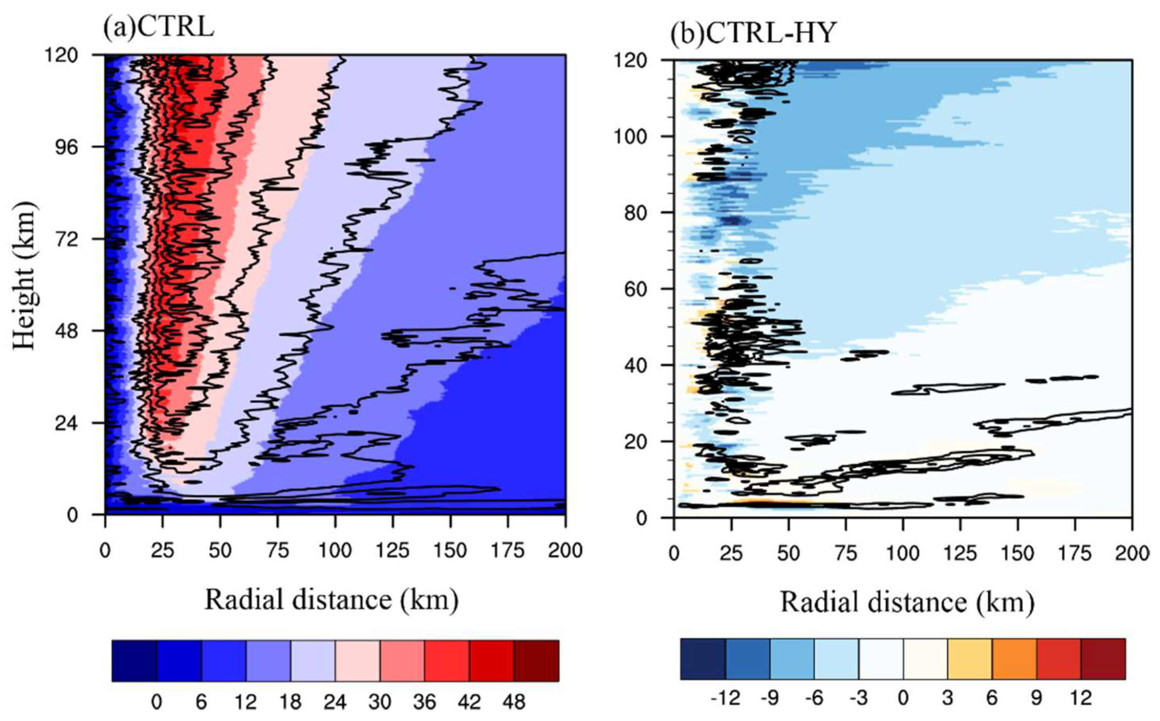
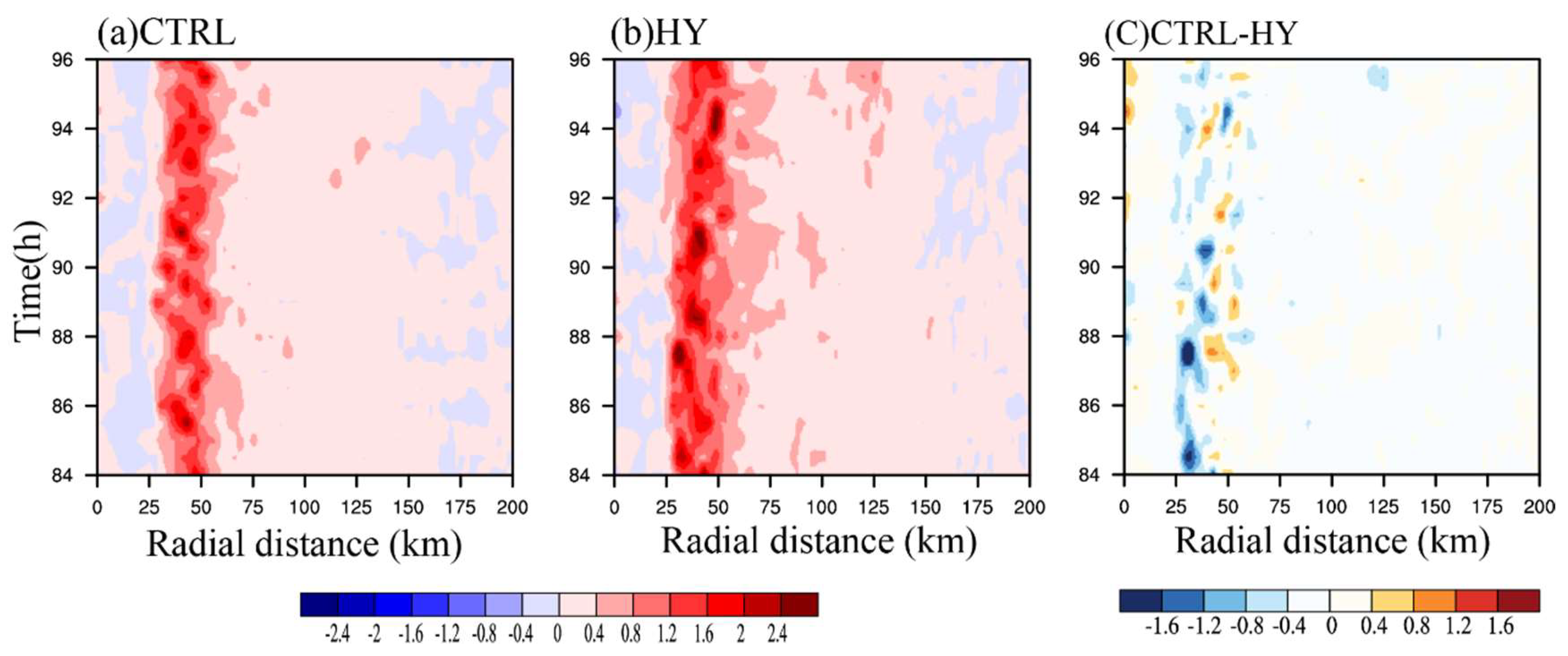
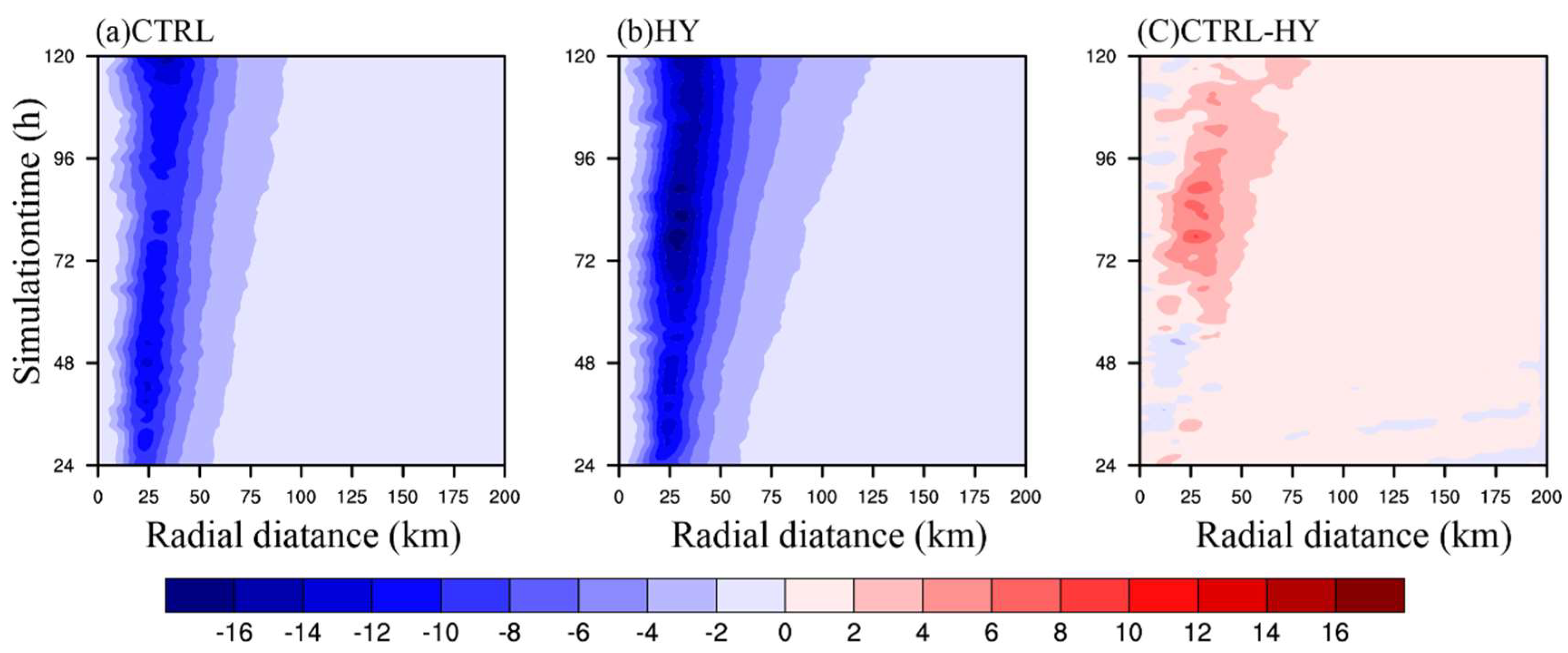
Figure 3 displays the time evolution of the 10-m tangential winds in CTRL and the differences between CTRL and HY. The maximum tangential wind in CTRL is maintained at the radius of about 35 km in the mature stage (Figure 3a). Their difference (Figure 3b) indicates that the tangential wind field in the CTRL eyewall region is mostly weaker than in HY during the evolution of the intensity of the TCs. After 24 h, the 10-m tangential wind field in HY is significantly enhanced in the outer region. In the study of the maximum difference in TC intensity between 84 and 96 h, the 10-m tangential wind field in the eyewall region in CTRL is remarkably weaker than in HY (Figure 3b), which is associated with the smaller low-level inflow in the boundary layer in CTRL (Figure 2). This suggests that the influence of the hydrostatic assumption is significant in relation to TC intensity and that nonhydrostatic processes lead to weaker TC intensity.

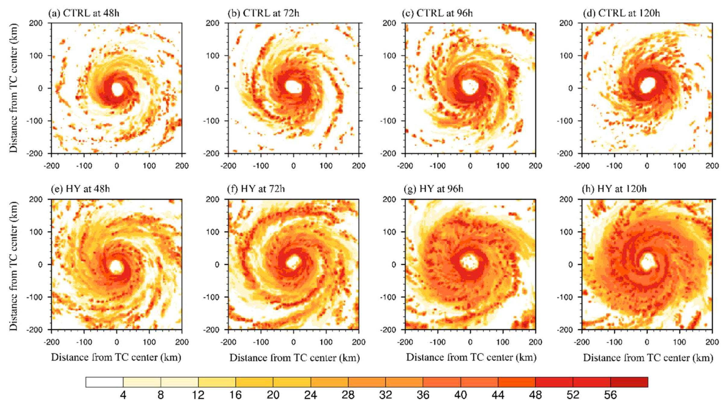
Figure 4 shows snapshots of the simulated maximum radar reflectivity for CTRL and HY at 24-h time intervals. The quasiperiodic behavior of the rainbands leads to a variation in activity and fluctuation of the inner and outer rainbands [30]. The inner and outer rainbands of the storm in CTRL are active throughout its lifetime. At the early stage (24 h), the inner rainbands around the eyewall in CTRL are thin and the outer rainbands are weak (not shown). With the further intensification of the storm (Figure 1), the inner and outer rainbands develop steadily, i.e., the eyewall thickens and the rainbands become more widely distributed. As the convection of the rainbands strengthens, the size of the storm increases (Figure 1c). Subsequently, the outer convective cells gradually move inward and merge, and the intensity of the TC increases rapidly (Figure 1a). A complete convection ring forms on the outside of the inner eyewall, wrapped outside the original eyewall. In HY, the eyewall convection and inner rainbands are also active, but the characteristics of the outer rainbands exhibit agreat discrepancy relative to those in CTRL. Between 48 and 72 h, the spiral structure in HY is more pronounced than CTRL, which suggests that the outer rainbands are more active. At 96 h, the eyewall becomes much thicker than CTRL. The outer rainbands in HY throughout the simulation are consistently more active and cover a larger region than in CTRL (Figure 4).

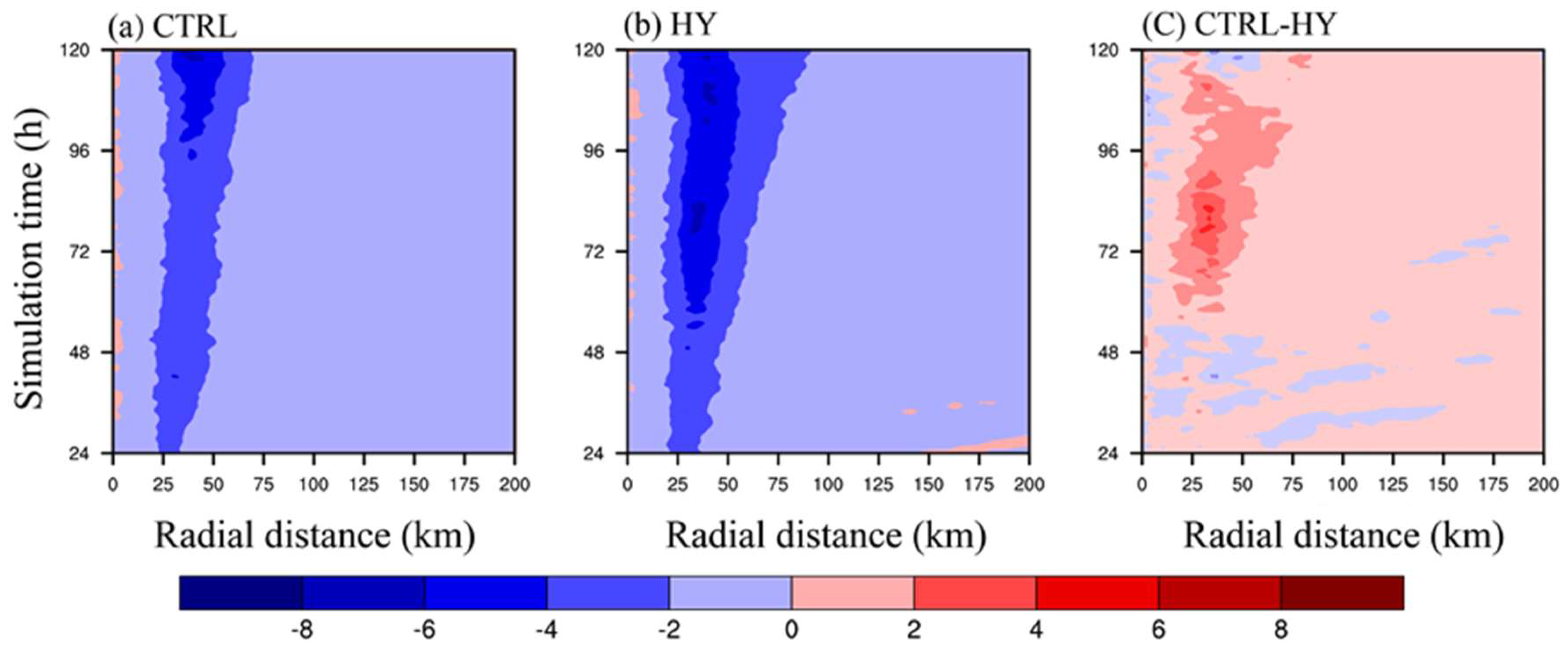
To better illustrate the difference of the vertical motion between CTRL and HY, the evolution of the vertical winds is shown in Figure 5. In the eyewall with a radius of 30–60 km in the mid-troposphere (6 km), the convection in CTRL is strong, while the outer regions have weaker convection. However, when the hydrostatic dynamical core is used, the range of convection in the eyewall extends to the radius of 75 km. Convection in the eyewall show significant differences between CTRL and HY. At the inner side of the eyewall, the convection in HY is more active than in CTRL, while at the outer side of the eyewall (radius of approx. 50 km), the convection is stronger in CTRL than in HY. This might occur because the eyewall in CTRL is tilted further outward with height than in HY (Figure 2a).

3.2. Vertical Momentum Budget

The vertical momentum budget is analyzed to elucidate the differences in the intensity and structure of the TCs between the CTRL and HY runs. In the WRF model, a reference state that is a function of height only is defined. To compute the vertical acceleration term in the vertical momentum equation, we first calculate the buoyancy and pressure perturbations based on this reference state. Perturbation quantities are derived by subtracting the reference-state value. The buoyancy force is not unique in the sense that it depends on the arbitrary choice of a reference density distribution; however, the sum of the buoyancy force and the perturbation pressure gradient is unique [31].

The definition of the reference state is intended to separate the balanced state from any locally unbalanced disturbances. The conventional wisdom for isolated convection suggests that the hydrostatic balance dominates and that the reference state can be represented satisfactorily by the horizontally homogeneous clear air within a few hundred kilometers of the convection [32]. TCs are rapidly rotating entities, and their convection, which is superimposed on a slowly evolving lateral circulation, is dominated by both the hydrostatic balance and the horizontal gradient wind balance. Therefore, the adoption of an appropriate method for defining the reference state is important. The reference state is defined by a running average using four neighboring points on constant σ surfaces [21]. The low-wavenumber (0 and 1) storm structure was used here to define the reference state [33], and a running Bartlett filter was applied to define the local reference state [32].

In this study, the reference state was defined following Zhang et al. [21]. First, a reference virtual temperature field ($T_{\mathrm{v}}$) is obtained by performing a running average on the model output data using four neighboring points on constant $\eta$ surfaces. Second, a reference pressure ($p$) is calculated by integrating the hydrostatic equation. The gas law ($p=\rho RT$, where $R$ is the specific gas constant) is used to calculate a reference $\rho$. The reference-state variables are therefore functions of $(x,y,\eta ,t)$. In this manner, the perturbation pressure, perturbation virtual temperature, and perturbation air density are given by

$$\begin{array}{l}{p}^{\prime }(x,y,\eta ,t)=p(x,y,\eta ,t)-\overline{p}(x,y,\eta )\\ T_v^{\prime }(x,y,\eta ,t)=T_v(x,y,\eta ,t)-{\overline{T}}_v(x,y,\eta )\\ {\rho }^{\prime }(x,y,\eta ,t)=\rho (x,y,\eta ,t)-\overline{\rho }(x,y,\eta )\end{array}$$

(4)

Because mature TCs are axisymmetric to a certain degree, we discuss the inner-core dynamics using cylindrical coordinates ($r,\lambda ,z$), where r is the radius from the vortex’s minimum pressure pointing outward, $\lambda$ is the azimuthal angle, and z is height. The vertical momentum equation is used to identify the causes of the difference in upward motion between the CTRL and HY runs, which can be written as follows [21]

$$\begin{array}{l}\frac{dw}{dt}=-\frac{1}{\rho }\frac{\partial p^{\prime }}{\partial z}+g(\frac{\overline{\rho }}{\rho }\frac{T_V{}^{\prime }}{T_V}-\frac{P^{\prime }}{P})\\ -g(q_c+q_r+q_i+q_s+q_g)\\ +2\mathsf{\Omega }{u}_m\cos (\varphi )+D_W\end{array}$$

(5)

where

$$\frac{d}{dt}=\frac{\partial }{\partial t}+U\frac{\partial }{\partial r}+\frac{V}{r}\frac{\partial }{\partial \lambda }+W\frac{\partial }{\partial z}$$

(6)

In the above, U, V, and W denote the radial, tangential, and vertical winds in cylindrical coordinates, respectively. The five terms on the right-hand side of Equation (5), which determine the quantity of vertical acceleration following a parcel, include the vertical perturbation pressure gradient force (denoted PGF), local buoyancy force (denoted LBF) containing the thermal and dynamic buoyancy relative to the surrounding environment, water loading (WL), Coriolis effects (WC), and diffusion effects (WD). The subsequent discussion treats the Coriolis and diffusion effects in combination (denoted as WCD).

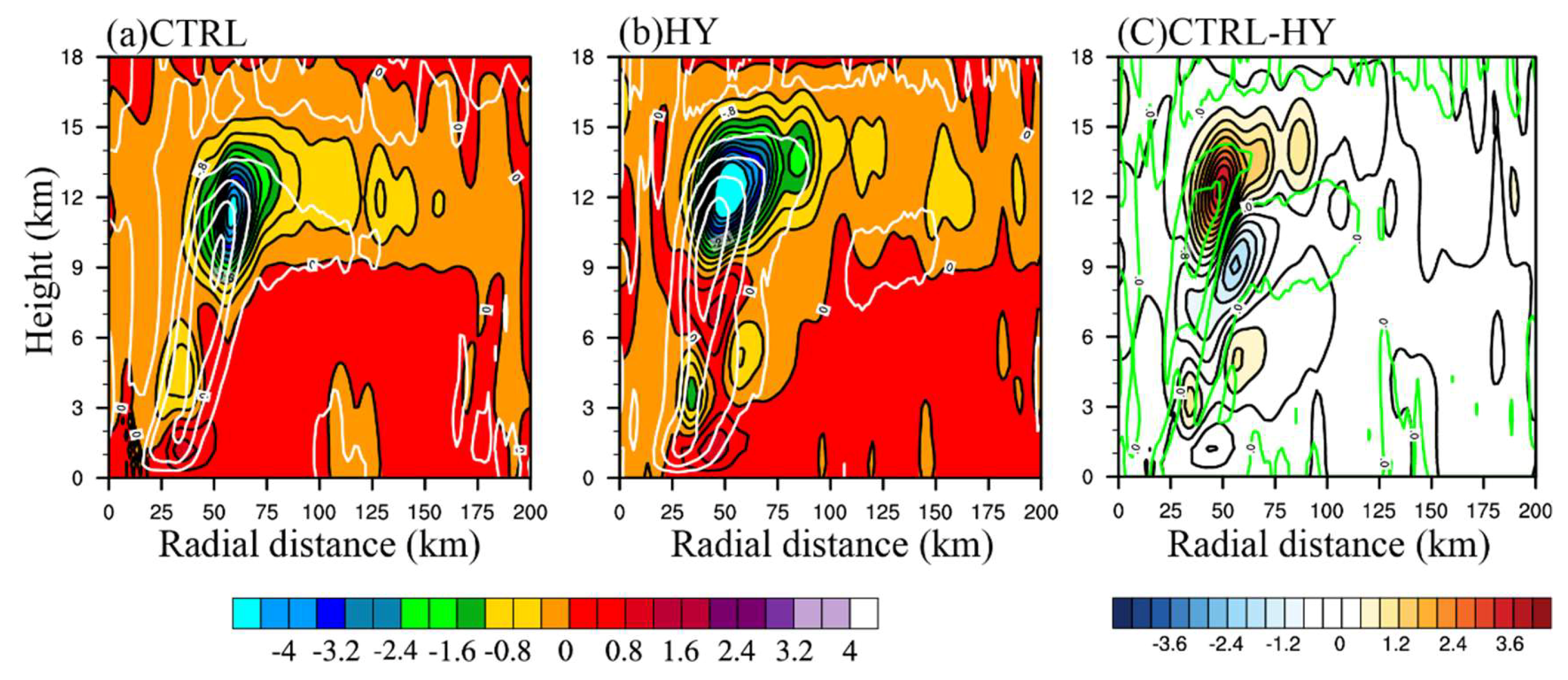
Figure 6 displays the azimuthally averaged vertical acceleration of vertical wind for the CTRL and HY runs as well as their differences. The total vertical acceleration in both runs is positive at the middle and lower eyewall regions and the largest values appear at the height of approximately 1 km. The magnitude of the vertical acceleration in CTRL first decreases and then increases with height, and the sign changes at the level of the maximum upward wind. The maximum positive acceleration is consistent with the PGF, indicating that the PGF plays an important role in lifting convection in the eyewall (Figure 7a). The LBF and WL are shown to both make major contributions to the formation of the negative peak vertical acceleration (Figure 7). Outside the eyewall, the acceleration tends to decrease. It is worth noting that negative acceleration occurs down to the height of 3 km in the eye. At the inner edge of the eyewall, there is a region of large negative acceleration at 3–6 km, which indicates it might be advantageous to include the effects of the drag of hydrometeors in calculating the vertical acceleration.

The vertical acceleration in HY has a similar structure to that in CTRL. The maximum vertical wind occurs at the height of about 10 km in the eyewall. Below this level, the vertical acceleration is positive and there are two larger centers in the eyewall. There is also a region of large negative acceleration in the eyewall at 3–6 km. In this region, the drag effects in HY appear stronger than in CTRL, resulting in the decrease in vertical acceleration and the smaller vertical velocity. A region of negative acceleration exists above the level of approximately z = 10 km.

The differences between the two runs indicate that the value of vertical acceleration in the eyewall in HY is greater than in CTRL, except for the region at 3–6 km in the inner core. A budget analysis suggests that a stronger WL in HY than in CTRL is responsible for such a difference (Figure 8). The results suggest that the greater involvement of clouds in this region contributes to enhanced effects of hydrometeor drag in HY. The combination of LBF and WL means the negative vertical acceleration in HY extends to a greater height than in CTRL. The vertical acceleration in the outer region in HY is generally slightly stronger than in CTRL, resulting in a strong updraft outside the eyewall.

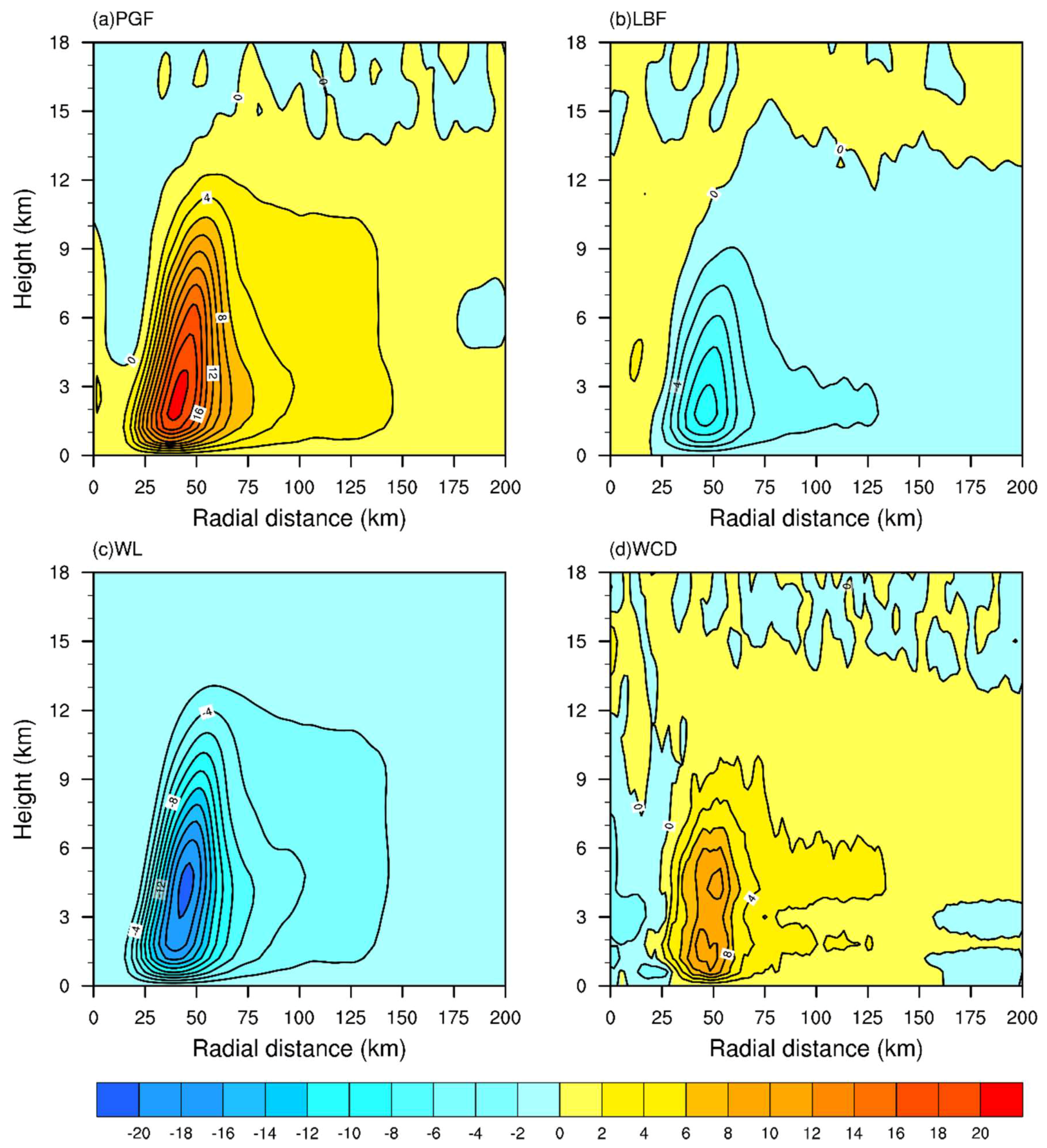
Figure 7 depicts four budget terms in Equation (2). In CTRL, the largest term of PGF (Figure 7a) is positive in the eyewall and the outer precipitation regions. However, it is negative in the eye down to 3 km. WL displays a similar structure but the opposite sign to PGF, with negative values in both the eyewall and the outer rainbands (Figure 7c). Relative to PGF and WL, LBF and WCD are two smaller terms. Local buoyancy is dominated by positive buoyancy in the eye and negative buoyancy in the eyewall (Figure 7b). The implication is that PGF tends to force relatively “colder” air to ascend in the eyewall and relatively “warmer” air to descend in the eye. The ascending parcels in the eyewall are therefore negatively buoyant [21] (Zhang et al., 2000). Comparing PGF (Figure 7a) with LBF (Figure 7b) reveals that PGF has a significantly stronger effect than LBF on vertical acceleration. The PGF can completely offset the LBF and has a relatively large residual. The maximum value of PGF exceeds 20 (${10}^{-3}$ ${\mathrm{m}\mathrm{s}}^{-2}$) and is of the same order in WL, suggesting that WL also plays an important role in vertical acceleration (Figure 7c). This result indicates that the effects of WL should be included in the eyewall when the hydrostatic balance is used to estimate the surface pressure of TCs. The WCD also contributes positively to the acceleration of vertical motion in the eyewall (Figure 7d), as reported in Zhang et al. [21].

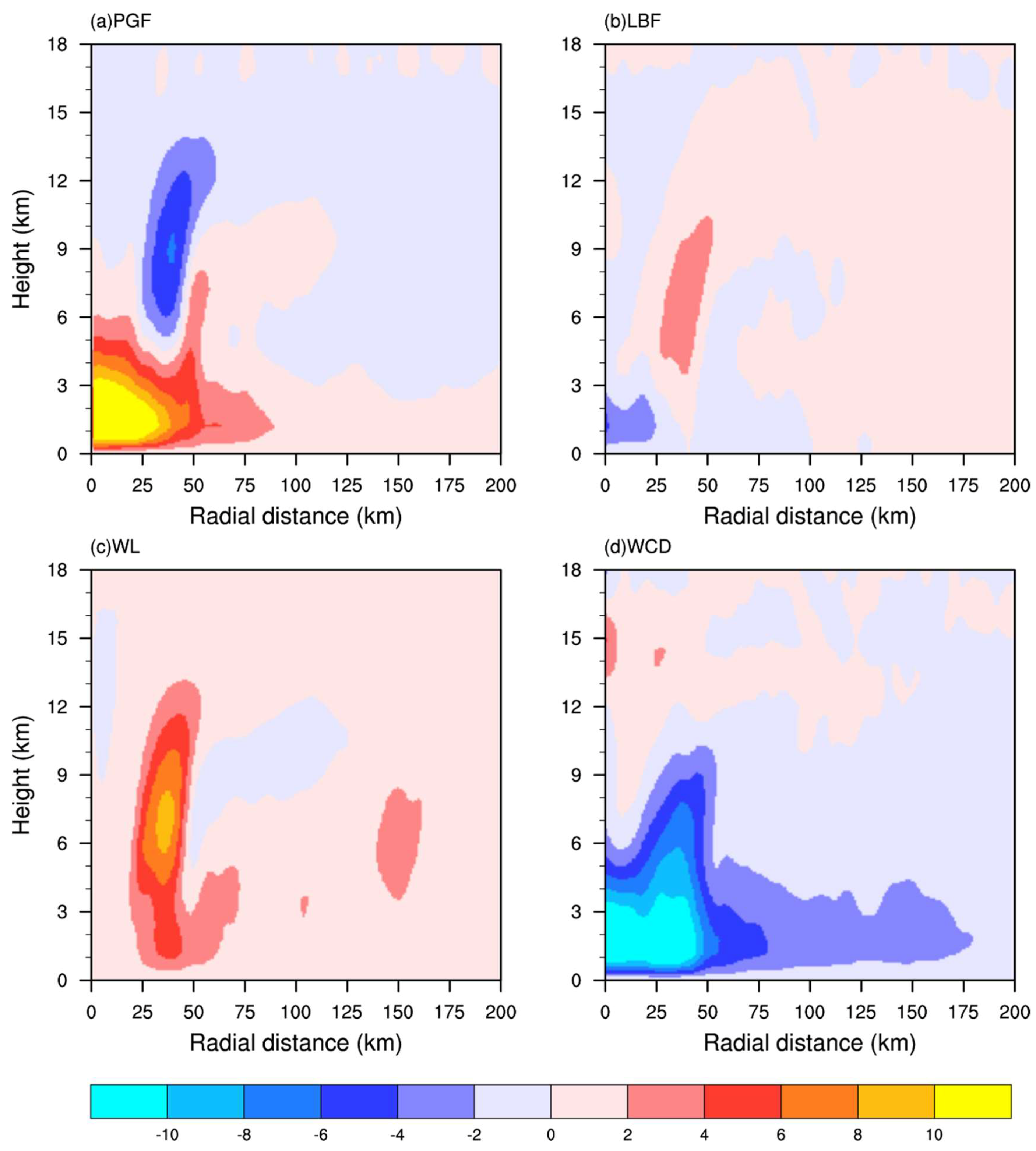
Figure 8 displays the differences between the CTRL and HY runs for all the budget terms in Equation (2). The PGF in HY is negative in the eye (not shown). Below the melting level (near 5 km) in the eye and in the eyewall, positive differences indicate that the PGF (Figure 8a), which plays a dominant role in lifting convection in the eyewall, is greater in CTRL than in HY. Above the melting layer, the PGF in HY is stronger than in CTRL, which results in the vertical winds reaching a greater height, i.e., approximately 15 km (Figure 2b). The difference in LBF (Figure 8b) shows the opposite characteristics to PGF. Below 3 km, LBF is negative in the eye. In the outer region, the differences between the two runs are also the opposite of the PGF. In HY, the larger LBF in the eyewall region corresponds to the stronger PGF, which suggests that the stronger vertical PGF imbalance will be offset by local buoyancy.

As stated above, the drag effects of WL cannot be ignored when calculating vertical acceleration. The difference of WL is presented in Figure 8c, which shows that the differences between CTRL and HY in the eyewall and outer rainband regions at low levels are positive, suggesting that WL in the eyewall is notably stronger in HY than in CTRL. In HY, the weaker PGF at lower levels and the stronger effects of WL result in the stronger negative vertical acceleration at the height of 3–6 km in the eyewall region (Figure 6b). The positive difference in the eyewall indicates that the drag effect in HY is more pronounced than in CTRL. Note, in the eyewall, the differences in both LBF and WL between CTRL and HY are positive (Figure 8b), whereas they are negative for PGF above 5 km (Figure 8a). This indicates that the imbalance induced by the more intense vertical PGF in the eyewall region is balanced by the stronger WL and LBF. The difference of WCD is shown in Figure 8d. Below about 5 km in the eyewall, WCD is negative. The stronger WCD at low levels in HY contributes to the larger acceleration of vertical motion in that region (Figure 6c). Above about 5 km, WCD is positive in the eyewall, which indicates that WCD is weaker in HY than in CTRL.

The above budget analysis indicates that the stronger vertical PGF is the most important factor in inducing the stronger vertical acceleration in HY, which leads to increased convective activity in the eyewall. This stronger convection causes both the low-level inflow and the high-level outflow to increase, which results in stronger tangential winds (Figure 2b) and, consequently, a more intense storm. These results underscore the importance of the vertical imbalance generated by the vertical perturbation pressure force, local buoyancy, and water loading.

3.3. Tangential Wind Tendency Equation Budget

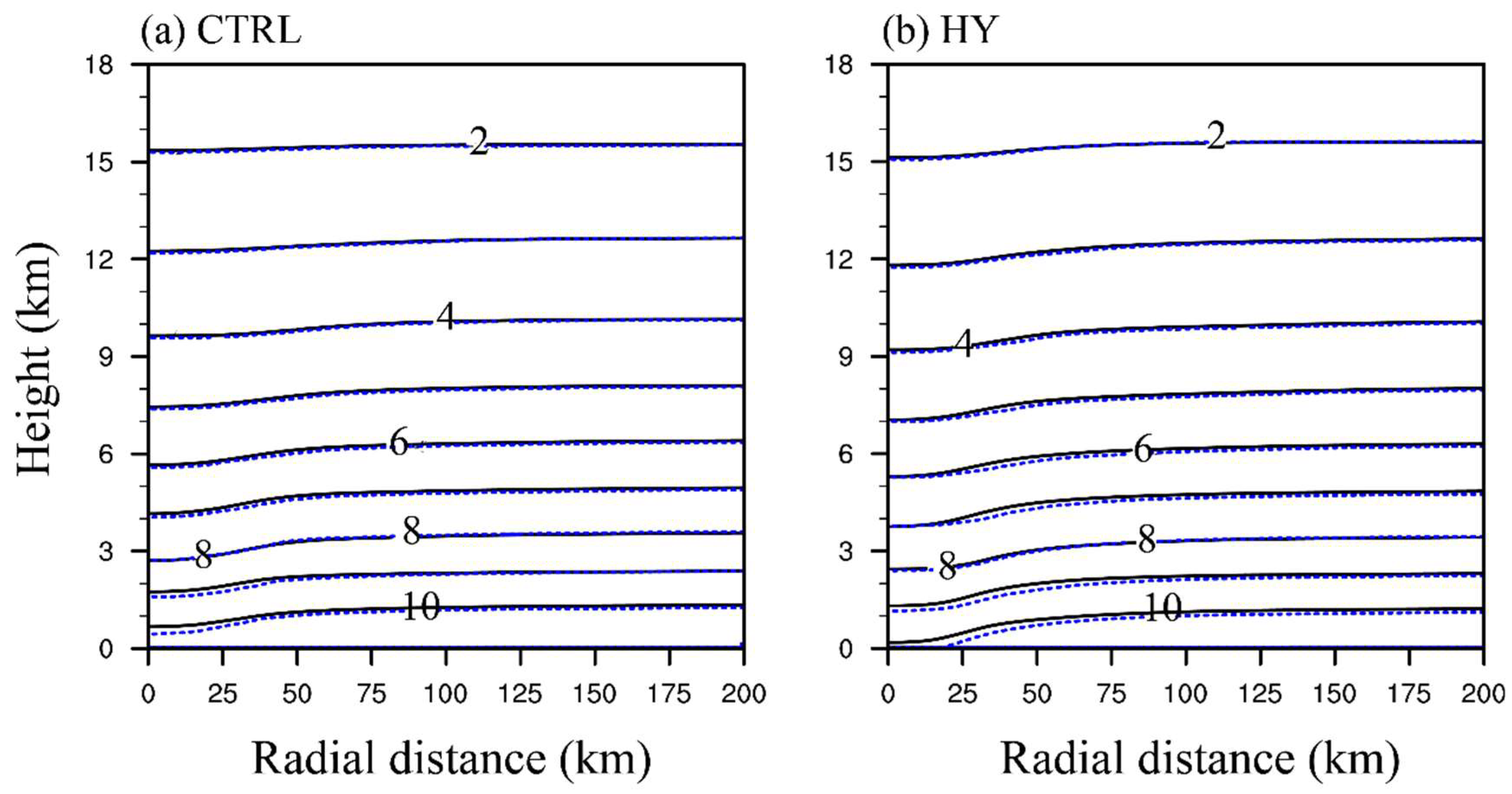
To further explain why the hydrostatic simulation develops a larger vertical motion than in the CTRL, we display in Figure 9 the height–radius cross-sections of the equivalent potential temperature (${\theta }_e$) and absolute angular momentum (AAM). The AAM in CTRL and HY decreases with height in the inflow layer, but increases with height in the outflow layer. The eyewall regions consist of densely inclined AAM contours, flattening in the upper outflow layer in both CTRL and HY. In the saturated eyewall, the AAM surfaces are almost parallel to the equivalent temperature ${\theta }_e$, indicating the existence of a conditionally symmetric neutral [34]. In the TC environment, the potential instability is strong. The AMM is stronger in hydrostatic storm than in nonhydrostatic simulations, suggesting more potential instability, and the larger AAM is transmitted inward in the lower inflow layer, which promotes a larger tangential wind speed. In the lower inflow layer, the ${\theta }_e$ both in HY and CTRL increases rapidly inward and reaches a maximum at the lower TC center. 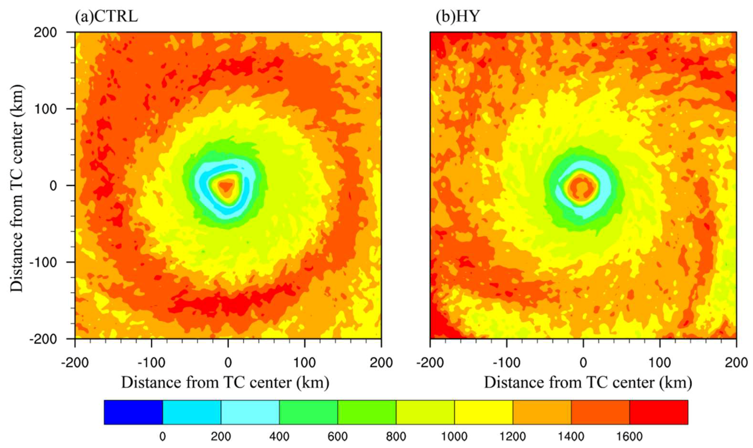In the upper troposphere, the ${\theta }_e$ rises sharply, the relatively low value appears in the middle and outer regions of the troposphere, and the low-value region is separated by the high-energy updraft that is transported upward by the boundary layer in the eyewall regions. The horizontal distribution of maximum CAPE in Figure 10 indicates considerable CAPE in the storms’ environment, Consistent with the large potential instability in the ambiance of the hurricane. The higher-${\theta }_e$ air with more potential instability or convective available potential energy (CAPE) in the eyewall regions in HY indicates a stronger dynamic lifting resulting from the larger inflow in boundary layer.

The simulated TC has significant differences in convection both in the eyewall and the secondary circulation. The tangential wind is stronger in HY than CTRL, and a larger and stronger TC was formed. To analyze the differences in storm size and intensity between CTRL and HY, we diagnosed the tangential wind tendency equation, which can be written as [35,36]

$$\begin{array}{l}\frac{\partial \overline{v}}{\partial t}=(-\overline{u}\frac{\partial \overline{v}}{\partial r}-\overline{u}\frac{\partial \overline{v}}{\partial r}-f)+(-\overline{w}\frac{\partial \overline{v}}{\partial z})\\ +(-\overline{u^{\prime }\frac{\partial v^{\prime }}{\partial r}}-\overline{u^{\prime }\frac{\partial v^{\prime }}{\partial r}}+\overline{w^{\prime }\frac{\partial v^{\prime }}{\partial z}})+\overline{Diss}\end{array}$$

(7)

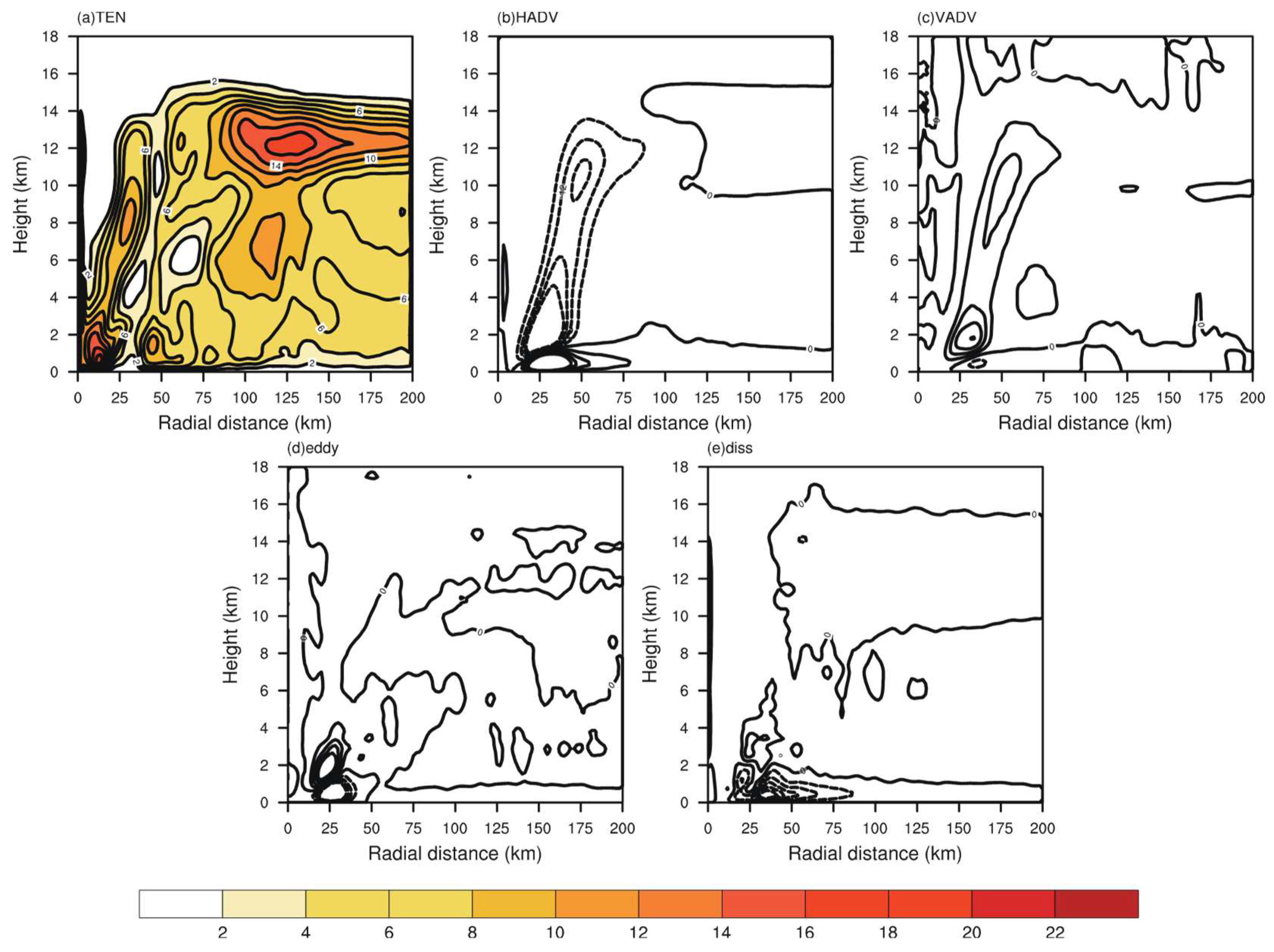
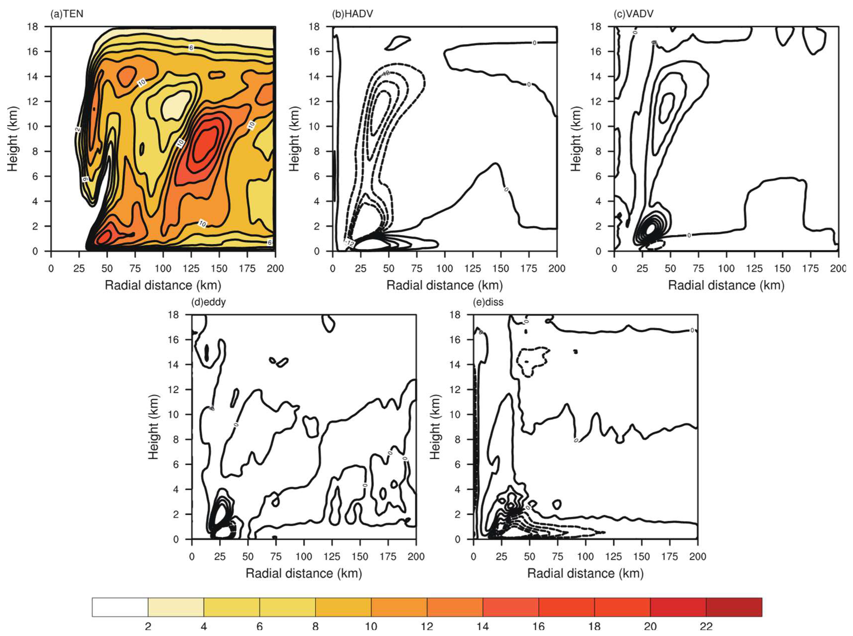
where f is the Coriolis parameter, and DISS is the surface friction and diffusion which is derived as a residual of Equation (7). The four terms on the right-hand side which determine the quantity of the azimuthally averaged tangential wind tendency (donated as TEN) include the horizontal advection (denoted as HADV), vertical advection (denoted as VADV), the eddy advection (denoted as eddy), and the surface friction and diffusion effects (DISS). The tangential wind tendency and all budget terms are compared in Figure 11 and Figure 12 for CTRL and HY. The HADV is shown as the only positive quantity in the boundary layer, indicating the inward transmission of absolute angular momentum that spins up the TC. Above the boundary layer, radial advection mainly contributes negatively to the tangential wind, while vertical advection produces a positive contribution. The contribution of the eddy processes is significant in the low-level eyewall regions. The surface friction mainly consumes the absolute angular momentum, but it also applies an inward force on the airflow [4]. For CTRL, the increase of tangential winds in TC is most pronounced in the top outflow layer. The increase of tangential winds in the inner-core regions is relatively smaller than the outflow layer, which is related to a large negative HADV above the boundary layer. The increase of tangential wind in the outer regions is notable, which is mainly due to the non-adiabatic heating of the eyewall and the outer rainbands [5]. Compared with CTRL, the increase of tangential winds in the eyewall and the outer rainband is slightly stronger in HY, and there is a similar structure in the tangential winds. In addition, in the eyewall and the 100-150 km radius regions, the tangential wind strengthening rate is significantly greater than CTRL, which indicates that the outer rainbands are more active in HY. The results indicate that the stronger non-adiabatic heating in the outer rainbands in HY result in a stronger increase of tangential winds, which contributes to a more intense and larger storm.

3.4. Explanation of the Hydrostatic Balance

Following on from the previous discussion, if we ignore the water loading, Coriolis force, and numerical diffusion, the vertical acceleration can be written as

$$\frac{Dw}{Dt}=\frac{1}{\rho }\frac{\partial p}{\partial z}-g$$

(8)

Although the structure of the vertical acceleration in the eyewall is well organized in both HY and CTRL, the hydrostatic balance is satisfied approximately in the TCs (Figure 13). A somewhat surprising feature is that when using the hydrostatic dynamic core, the hydrostatic balance is still not strictly met. The vertical acceleration in the eyewall is greater in HY than in CTRL (Figure 7c). This is consistent with the results shown in (Figure 13), whereby the vertical pressure gradient and gravity difference in the eyewall region is slightly larger in HY than in CTRL.

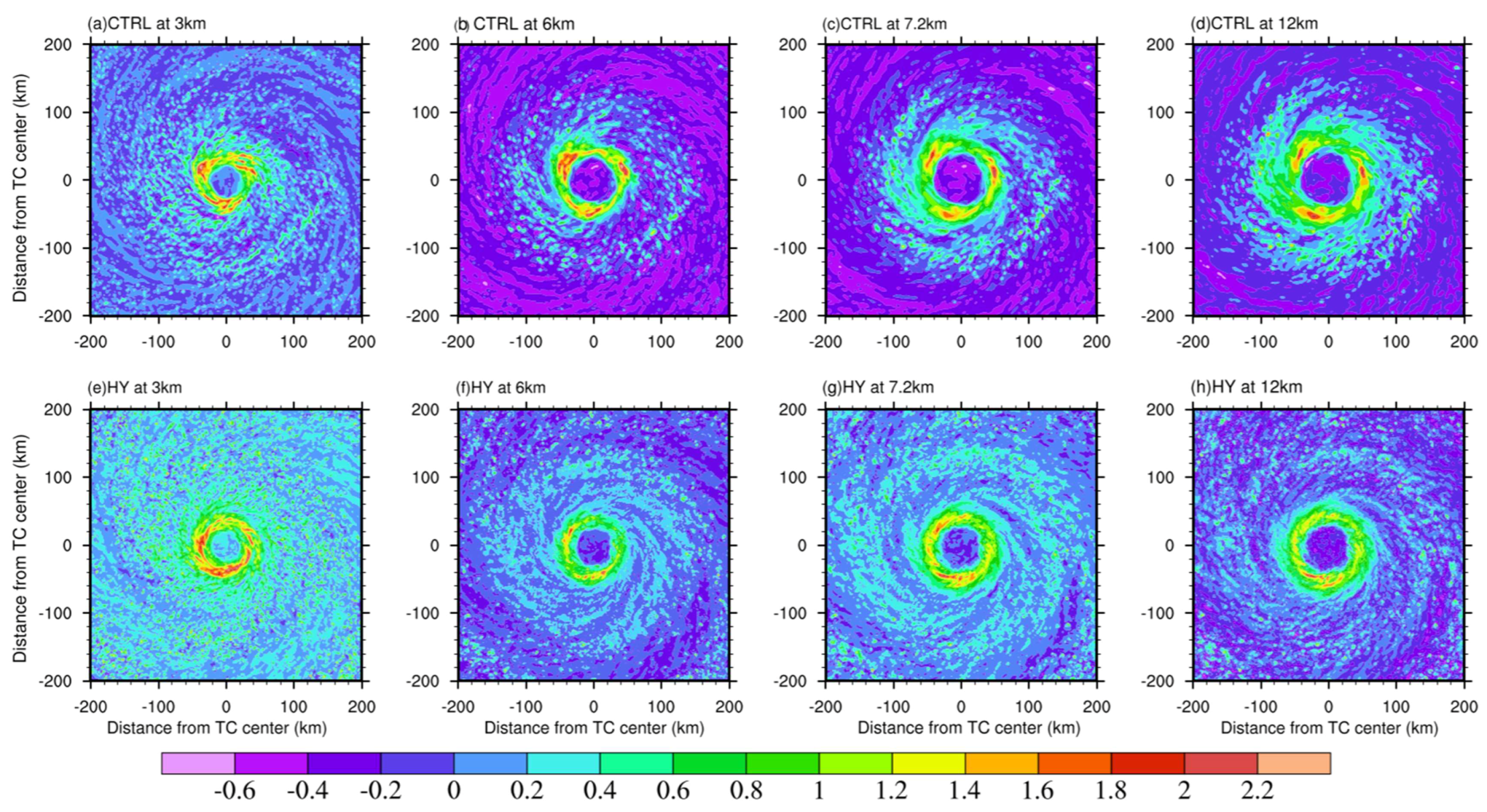
The horizontal distribution of vertical winds at different heights (Figure 14) shows the largest difference between HY and CTRL. The outer rainbands are more active in HY, which is linked to the stronger vertical acceleration in HY at the outer region (Figure 6c). At 3 km, there is significantly stronger convection in the eyewall in both CTRL (Figure 14a) and HY (Figure 14a). However, the convection in CTRL is always slightly stronger than in HY, which is consistent with the larger vertical acceleration at the lower levels of the eyewall in CTRL (Figure 6c). At 6 km, a local ascending motion in the eyewall structure is stronger in CTRL than in HY; however, the eyewall is more contracted and more symmetrical in HY than in CTRL (Figure 14b,f). On the 6-km height plane, the evolution of vertical winds over time (Figure 5b) shows that the difference between CTRL and HY at the radius of 25–60 km has both positive and negative regions, and that the positive region is attributed to the shrinkage of the eyewall in HY. Moreover, at the outer region, the ascending motion is stronger and extends over a greater region in HY than in CTRL.

At 9 km, the characteristics in the eyewall are approximately the same as those at 6 km. Convection in the outer region in HY is significantly more active than in CTRL, which is because the positive vertical acceleration in HY at the outer region is significantly greater than in CTRL (Figure 6c). At 15 km in CTRL, the eyewall structure disappears and upward motion is not evident (Figure 14d). Conversely, in HY, the eyewall structure remains obvious and the vertical winds in the eyewall are significantly greater than in CTRL (Figure 14h). These results show that convection at the eyewall region is stronger in HY than in CTRL and that the vertical winds in HY can reach a greater height, which is consistent with the larger vertical acceleration (Figure 6b).

3.5. Dynamic Mechanisms and Thermal Mechanisms of TCs

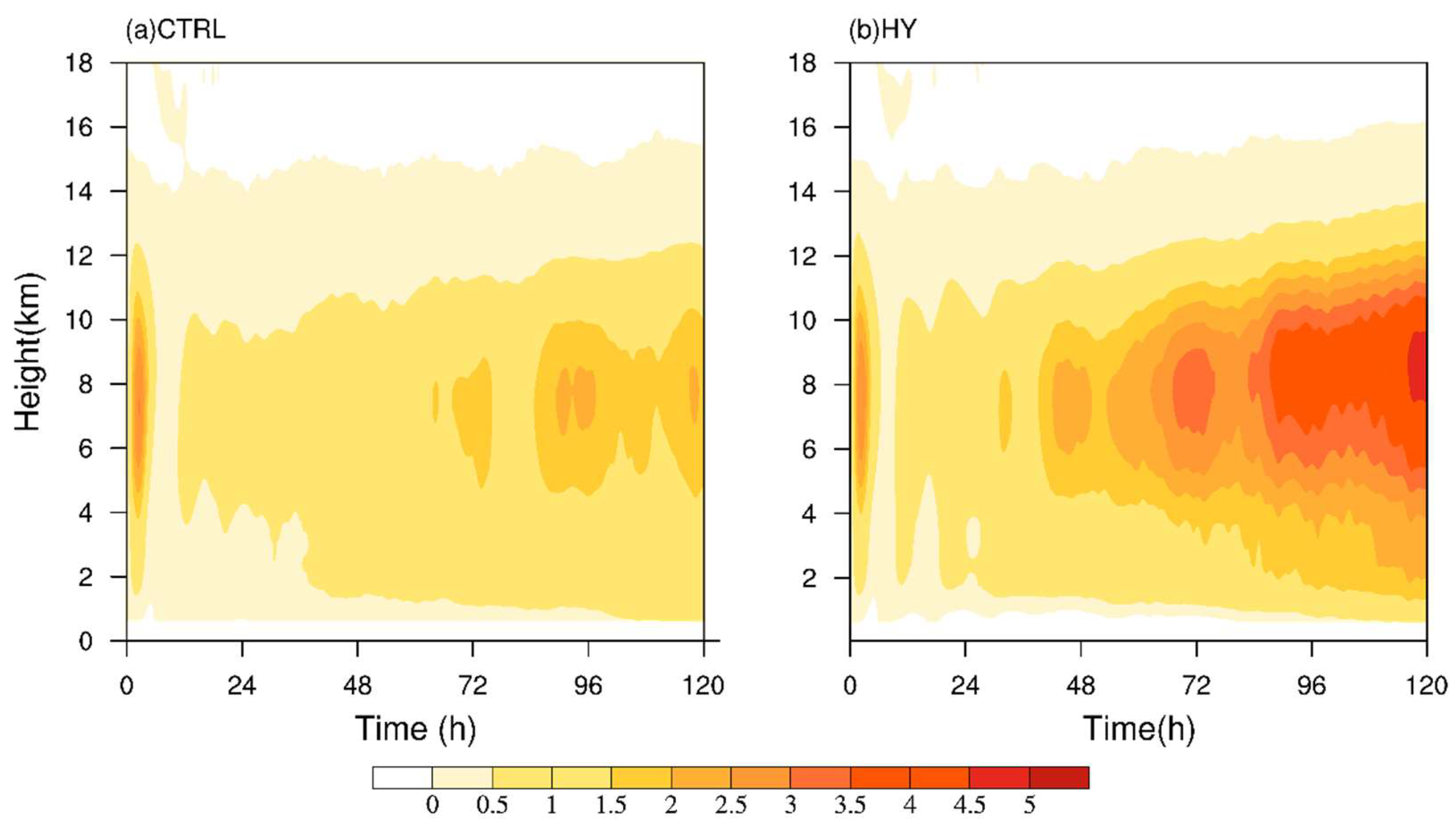
To elucidate the processes associated with the contraction of the eyewall in HY, we consider the inherent dynamic and thermal mechanisms. Latent heat release, which is closely related to convection in the eyewall and the secondary circulation of the TC, is also a source of energy for maintaining and developing TC intensity. Figure 15 depicts the time evolution of the azimuthal mean latent heat release. Latent heat release begins at the lifting condensing level. In CTRL, the latent heat release is small at the beginning of TC development, although it becomes larger after about 12 h. As the TC intensity increases, the release of latent heat becomes even larger at 72 h, and it is especially pronounced at the height of 5–10 km (Figure 15a). The structure of latent heat in HY is similar to CTRL. The main difference is that the magnitude of the release of latent heat in HY is notably greater than in CTRL, which results in enhanced TC intensity starting from approximately 48 h (Figure 1).

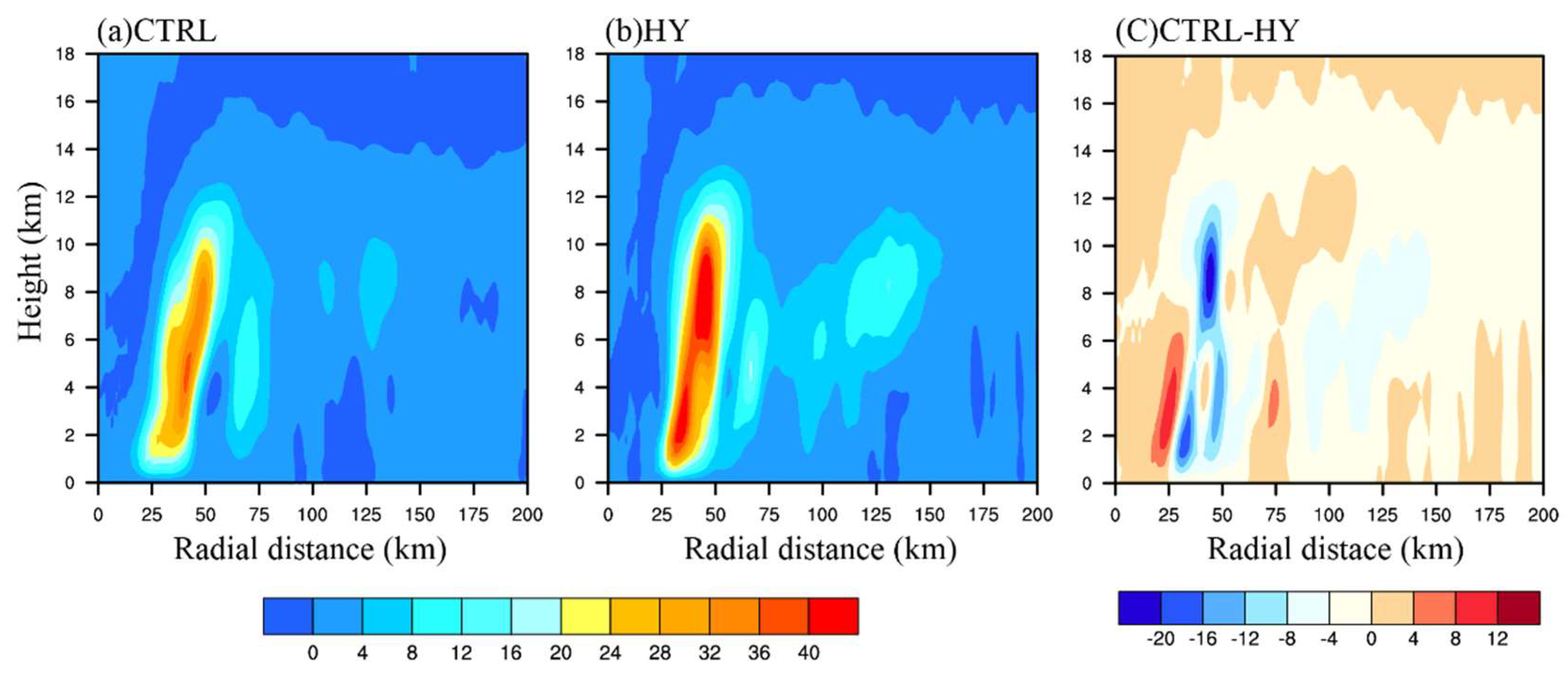
Figure 16 exhibits height–radius cross-sections of the azimuthal mean latent release in the two runs as well as their difference. The latent heat release in both CTRL and HY is pronounced in the eyewall and the maximum is concentrated at the height of about 8 km (Figure 16a,b). The structure of the latent heat release is consistent with the structure of the distributions of the vertical and horizontal wind vectors (Figure 2). The location of latent heat release closer to the center of a TC is more conducive to the reduction of the central pressure [37]. In the previous sections, we discussed the inward contraction of the eyewall in HY. Our results indicate that the latent heat release in the eyewall is stronger and closer to the TC center in HY than in CTRL (Figure 16c), which contributes to the reduction of the central pressure and leads to the significantly greater TC intensity in HY than in CTRL (Figure 1). Because of this, the pressure gradient force will increase, which will then change the net radial force.

Figure 17 displays the time evolution of the radial pressure gradient in the CTRL and HY runs as well as their differences. The pressure gradient for both runs is most significant near the eyewall region, where the convection is most active and the pressure deepens inward rapidly [38]. The outer rainbands, which are more active in HY than in CTRL, cause a larger pressure gradient radial range. From the difference between the two runs, it can be seen that the pressure gradient in HY is significantly larger than in CTRL in the eyewall region from about 48 h to the end of the simulation. This might be attributable to an increase in the release of latent heat in the eyewall region (Figure 16), which results in reduced central pressure and further increases the pressure gradient.

The net radial force, which is defined to evaluate the degree of gradient wind imbalance, can be written as follows [39]:

$$F=-\frac{1}{\rho }\frac{\partial p}{\partial r}+\frac{v^2}{r}+fv$$

(8)

Hovmöller diagrams of the net radial force for CTRL and HY as well as their differences are presented in Figure 18. The net radial force for both runs is significant in the eyewall region, but with stronger values in HY. The gradient wind imbalance in the eyewall region is significant. The negative radial force corresponding to the subgradient wind indicates a tendency to accelerate the inflow. The maximum net radial force in HY is 50% larger than in CTRL (Figure 18c), which should be attributable to the larger pressure gradient in HY (Figure 17c). This result indicates that the greater net radial force in HY causes the eyewall to contract inward, allowing latent heat release closer to the center of the TC. The greater release of latent heat (Figure 16b) is conducive to TC strengthening (Figure 1), which further leads to an increase of the radial pressure gradient of the eyewall (Figure 17). Such positive feedback causes the eyewall to contract, which leads to greater convective activity in the eyewall. In fact, as the pressure gradient increases, the tangential winds in HY will increase (Figure 2) to maintain the gradient wind balance [40].

To clarify the relationship between eyewall contraction and TC intensity, we present height–radius cross-sections of the azimuthal mean vertical winds and tangential winds in Figure 19. The eyewall in CTRL slopes outward with height, whereas the eyewall in HY shrinks inward in comparison with CTRL (Figure 19). Moreover, the tangential winds have a greater vertical extent in HY than in CTRL. The less slanted contours reflect the larger radial and tangential wind gradients, which are beneficial to increased TC intensity [41]. This suggests that the greater vertical wind of the eyewall in HY is related to the contraction of the eyewall and the more vertical tangential wind contours (Figure 19b). Meanwhile, the larger vertical motion leads to greater convective activity in the eyewall, which contributes to TC intensification.

4. Summary and Discussion

This study compared the influence of incorporating the hydrostatic or nonhydrostatic assumption in the WRF model on the intensity and structure of simulated TCs. The results indicated that the difference between the two dynamical cores is significant. When using the hydrostatic dynamical core, a TC has stronger intensity and a larger spatial scale. Furthermore, convection in the eyewall region is stronger, the eyewall shrinks inwardly, and the outer rainbands are more active. The greater convective activity in the eyewall region leads to a stronger secondary circulation accompanied by stronger inflow at the boundary layer and stronger outflow at higher levels, which result in the expansion of the tangential wind field.

The vertical force balance in the inner-core region was also investigated. The vertical momentum budget was analyzed to explain the differences between the two model runs, especially in the eyewall region. Results indicated that vertical acceleration undergoes significant differences in the eyewall and outer regions between the two runs. The hydrostatic simulation produced a stronger TC with a greater extent, mainly resulting from the stronger vertical perturbation pressure gradient, which leads to stronger upward acceleration in the eyewall. In this study, the small vertical acceleration was calculated based on the four large terms: PGF, LBF, WL, and WCD. The vertical acceleration was found to be four orders of magnitude smaller than the acceleration of gravity, which means that, irrespective of whether the hydrostatic or nonhydrostatic dynamical core is used, the hydrostatic balance is largely satisfied in the TC eyewall. The WL effects must be included in the hydrostatic equation when estimating the surface pressure in precipitation regions [21]. The tangential wind tendency equation budget indicated that the more latent heat in the hydrostatic storm results in a stronger increase in non-adiabatic heating, which is conducive to the increase of tangential wind, and finally forms a larger-scale TC compared with the nonhydrostatic simulation.

In lower and central portions of the eyewall, the perturbation PGF in the eyewall region plays an important role and causes the upward acceleration to increase. Larger positive acceleration in the eyewall was found in HY than in CTRL, which corresponds to the larger perturbation PGF. In particular, the impact of WCD, which has been ignored in some previous studies, should be included when calculating the vertical acceleration. Results indicated that when the hydrostatic dynamical core is used, the WCD in the eyewall region is weaker in HY than in CTRL (approximately above 6 km), which results in large vertical acceleration. The enhanced convective activity in the eyewall region in HY, in comparison with CTRL, contributes to a stronger secondary circulation, accompanied by enhanced low-level inflows and high-level outflows that eventually result in increased tangential winds.

When the hydrostatic dynamical core is used, the latent heat release in the eyewall region is stronger, which is beneficial to the reduction of the central pressure of the TC. This further results in an increase in the pressure gradient near the eyewall region. Meanwhile, the increase of the net radial force causes the TC eyewall to contract and the latent heat to be released closer to the TC center, which is conducive to reducing the central pressure. This positive feedback leads to an increase in the mass convergence at low levels in HY, which facilitates the further development of the convection.

References

1. Wedi, N.P.; Smolarkiewicz, P.K. A framework for testing global non-hydrosatic models. Q. J. R. Meteorol. Soc. 2009, 135, 469–484. [Google Scholar] [CrossRef]
2. Holton, J.R.; Hakim, G.J. An Introduction to Dynamic Meteorology; Academic Press: Burlington, MA, USA, 2012; 552p. [Google Scholar]
3. Gibbon, J.D.; Holm, D.D. Extreme events in solutions of hydrostatic and non-hydrostatic climate models. Philos. Trans. R. Soc. A 2011, 369, 1156–1179. [Google Scholar] [CrossRef] [PubMed] [Green Version]
4. Xu, L.; Raman, S.; Madala, R. A review of non-hydrostatic numerical models for the atmosphere. In Proceedings of the First World Congress of Nonlinear Analysis Fire and Forest Meteorology, Nonlinear World, Tampa, FL, USA, 19–26 August 1992. [Google Scholar]
5. Saito, K.; Ishida, J.-I.; Aranami, K.; Hara, T.; Segawa, T.; Narita, M.; Honda, Y. Non-hydrostatic atmospheric models and operational development at JMA. J. Meteorol. Soc. Jpn. 2007, 85, 271–304. [Google Scholar] [CrossRef]
6. Jang, J.; Hong, S.-Y. Comparison of simulated precipitation over East Asia in two regional models with hydrostatic and non-hydrostatic dynamical cores. Mon. Weather Rev. 2016, 144, 3579–3590. [Google Scholar] [CrossRef]
7. Tapp, M.; White, P.W. A non-hydrostatic mesoscale model. Q. J. R. Meteorol. Soc. 1976, 102, 277–296. [Google Scholar] [CrossRef]
8. Klemp, J.B.; Wilhelmson, R. The simulation of three-dimensional convective storm dynamics. J. Atmos. Sci. 1978, 35, 1070–1096. [Google Scholar] [CrossRef]
9. Yang, Q.; Leung, L.; Lu, J.; Lin, Y.; Hagos, S.; Sakaguchi, K.; Gao, Y. Exploring the effects of a non-hydrostatic dynamical core in high-resolution aquaplanet simulations. J. Geophys. Res. Atmos. 2017, 122, 3245–3265. [Google Scholar] [CrossRef]
10. Queney, P. The problem of airflow over mountains: A summary of theoretical studies. Bull. Am. Meteorol. Soc. 1948, 29, 16–26. [Google Scholar] [CrossRef]
11. Dalu, G.A.; Baldi, M.; Pielke, R.A., Sr.; Leoncini, G. Mesoscale non-hydrostatic and hydrostatic pressure gradient forces-theory. J. Atmos. Sci. 2003, 60, 2249–2266. [Google Scholar] [CrossRef]
12. Bubnová, R.; Hello, G.; Benard, P.; Geleyn, J.-F. Integration of the fully elastic equations cast in the hydrostatic pressure terrainfollowing coordinate in the framework of the ARPEGE/ALADIN NWP system. Mon. Weather Rev. 1995, 123, 515–535. [Google Scholar] [CrossRef]
13. Skamarock, W.C.; Klemp, J.B. A time-split non-hydrostatic atmospheric model for weather research and forecastingapplications. J. Comput. Phys. 2008, 227, 3465–3485. [Google Scholar] [CrossRef]
14. Dudhia, J. A non-hydrostatic version of the Penn State–NCAR mesoscalemodel: Validation tests and simulation of anAtlantic cyclone and cold front. Mon. Weather Rev. 1993, 121, 1493–1513. [Google Scholar] [CrossRef]
15. Kato, T. Hydrostatic and non-hydrostatic simulations of the 6 August 1993 Kagoshima torrential rain. J. Meteorol. Res. Jpn. Ser. II 1996, 74, 355–363. [Google Scholar] [CrossRef]
16. Janjić, Z.I.; Gerrity, J.P., Jr.; Nickovic, S. An alternative approach to non-hydrostatic modeling. Mon. Weather Rev. 2001, 129, 1164–1178. [Google Scholar] [CrossRef]
17. Saito, K.; Fujita, T.; Yamada, Y.; Ishida, J.I.; Kumagai, Y.; Aranami, K.; Ohmori, S.; Nagasawa, R.; Kumagai, S. The operational JMA nonhydrostatic mesoscale model. Mon. Weather Rev. 2006, 134, 1266–1298. [Google Scholar] [CrossRef]
18. Kato, T.; Saito, K. Hydrostatic and non-hydrostatic simulations of moist convection: Applicability of the hydrostatic approximation to a high-resolution model. J. Meteorol. Soc. Jpn. 1995, 73, 59–77. [Google Scholar] [CrossRef]
19. Dudhia, J. A history of mesoscale model development. Asia-Pac. J. Atmos. Sci. 2014, 50, 121–131. [Google Scholar] [CrossRef]
20. Jorgensen, D.P.; Zipser, E.J.; LeMone, M.A. Vertical motions in intense hurricanes. J. Atmos. Sci. 1985, 42, 839–856. [Google Scholar] [CrossRef]
21. Zhang, D.-L.; Liu, Y.; Yau, M.K. A multiscale numerical study of Hurricane Andrew (1992)—Part III: Dynamically induced vertical motion. Mon. Weather Rev. 2000, 128, 3772–3788. [Google Scholar] [CrossRef]
22. Skamarock, W.C.; Klemp, J.B.; Dudhia, J.; Gill, D.O.; Barker, D.M.; Duda, M.G.; Huang, X.-Y.; Wang, W.; Powers, J.G. A Description of the Advanced Research WRF Version 3; NCAR Tech. Note NCAR/TN-4751STR; National Center for Atmospheric Research: Boulder, CO, USA, 2008; 113p. [Google Scholar]
23. Lin, Y.-L.; Farley, R.D.; Orville, H.D. Bulk parameterization of the snow field in a cloud model. J. Clim. Appl. Meteorol. 1983, 22, 1065–1092. [Google Scholar] [CrossRef]
24. Dudhia, J. Numerical study of convection observed during the Winter Monsoon Experiment using a mesoscale two dimensional model. J. Atmos. Sci. 1989, 46, 3077–3107. [Google Scholar] [CrossRef]
25. Mlawer, E.J.; Taubman, S.J.; Brown, P.D.; Iacono, M.J.; Clough, S.A. Radiative transfer for inhomogeneous atmospheres: RRTM, a validated correlated-k model for the longwave. J. Geophys. Res. 1997, 102, 16663–16682. [Google Scholar] [CrossRef] [Green Version]
26. Hong, S.-Y.; Noh, Y.; Dudhia, J. A new vertical diffusion package with an explicit treatment of entrainment processes. Mon. Weather Rev. 2006, 134, 2318–2341. [Google Scholar] [CrossRef]
27. Kepert, J.D.; Wang, Y. The dynamics of boundary layer jets within the tropical cyclone core—Part II: Nonlinear enhancement. J. Atmos. Sci. 2001, 58, 2485–2501. [Google Scholar] [CrossRef]
28. Zhang, J.A.; Rogers, R.F.; Nolan, D.S.; Marksv, F.D. On the characteristic height scales of the hurricane boundary layer. Mon. Weather Rev. 2011, 139, 2523–2535. [Google Scholar] [CrossRef]
29. Houze, R.A. Clouds in tropical cyclones. Mon. Weather Rev. 2010, 138, 293–344. [Google Scholar] [CrossRef]
30. Li, Q.; Wang, Y. Formation and quasi-periodic behavior of outer spiral rainbands in a numerically simulated tropical cyclone. J. Atmos. Sci. 2012, 69, 997–1020. [Google Scholar] [CrossRef]
31. Smith, R.K. Buoyancy in tropical cyclone and other rapidly rotating atmospheric vortices. Dyn. Atmos. Oceans 2005, 40, 189–208. [Google Scholar] [CrossRef]
32. Eastin, M.D. Buoyancy of Convective Vertical Motions in the Inner Core of Intense Hurricanes—Part I: General Statistics. Mon. Weather Rev. 2004, 133, 188–208. [Google Scholar] [CrossRef]
33. Braun, S.A. A cloud-resolving simulation of Hurricane Bob (1991): Storm structure and eyewall buoyancy. Mon. Weather Rev. 2002, 130, 1573–1592. [Google Scholar] [CrossRef]
34. Emanuel, K.A. An air–sea interaction theory for tropical cyclones. Part I: Steady–state maintenance. J. Atmos. Sci. 1986, 43, 585–604. [Google Scholar] [CrossRef]
35. Bui, H.H.; Smith, R.K.; Montgomery, M.T.; Peng, J. Balanced and unbalanced aspects of tropical cyclone in-tensification. Q. J. R. Meteorol. Soc. 2009, 135, 1715–1731. [Google Scholar] [CrossRef] [Green Version]
36. Fudeyasu, H.; Wang, Y. Balanced contribution to the intensification of a tropical cyclone simulated in TCM4: Outer-core spinup process. J. Atmos. Sci. 2011, 68, 430–449. [Google Scholar] [CrossRef]
37. Hack, J.J.; Schubert, W.H. Nonlinear response of atmospheric vortices to heating by organized cumulus convection. J. Atmos. Sci. 1986, 43, 1559–1573. [Google Scholar] [CrossRef]
38. Ma, Z.; Fei, J.; Huang, X.; Cheng, X. Contributions of surface sensible heat fluxes to tropical cyclone—Part I: Evolution of tropical cyclone intensity and structure. J. Atmos. Sci. 2015, 72, 120–140. [Google Scholar] [CrossRef]
39. Smith, R.K.; Nguyen, V.S. Tropical cyclone spin-up revisited. Q. J. R. Meteorol. Soc. 2009, 135, 1321–1335. [Google Scholar] [CrossRef] [Green Version]
40. Gentry, M.S.; Lackmann, G.M. Sensitivity of simulated tropical cyclone structure and intensity to horizontal resolution. Mon. Weather Rev. 2010, 138, 688–704. [Google Scholar] [CrossRef]
41. Fierro, A.O.; Rogers, R.F.; Marks, F.D.; Nolan, D.S. The Impact of horizontal grid spacing on the microphysical and kinematic structures of strong tropical cyclones simulated with the WRF-ARW model. Mon. Weather Rev. 2009, 137, 3717–3743. [Google Scholar] [CrossRef]
Figure 1. Time series of the (a) minimum sea level pressure (hPa), (b) azimuthally averaged maximum surface (the lowest model level) wind speeds (m s−1), and (c) azimuthally averaged radius of hurricane-force (33 m s−1) winds (km).
Atmosphere 09 00483 g001
Figure 2. Height–radius cross-sections of the azimuthal mean tangential winds (color shaded, m s−1), radial winds (black contours, m   s 1 ), and vertical winds (green contours, m   s 1 ) for (a) the nonhydrostatic core (CTRL) and (b) hydrostatic core (HY) averaged between 84 h and 96 h. The vertical motion is shown with intervals of 0.4 m   s 1 , and the outmost contour is 0 m   s 1 .
Atmosphere 09 00483 g002
Figure 3. Time evolution of azimuthal mean 10-m tangential winds (color shaded, m   s 1 ), and radial winds (lines, m   s 1 ) for (a) CTRL, and (b) CTRL-HY (radial winds <−2   m   s 1 ).
Atmosphere 09 00483 g003
Figure 4. Plan views of the simulated maximum radar reflectivity (dBZ) between 24 and 96 h at intervals of 24 h for (ad) CTRL and (eh) HY, showing the evolutionary trend of rainbands.
Atmosphere 09 00483 g004
Figure 5. Time evolution of azimuthal mean vertical winds (color shade, m   s 1 ) for (a) CTRL, (b) HY and (c) CTRL-HY at 6 km in altitude, averaged between 84 and 96 h.
Atmosphere 09 00483 g005
Figure 6. Height–radius cross-sections of the azimuthal mean vertical accelerated   d w / d t (color shaded, m   s 1 h 1 ) and vertical winds (green contours, m s−1) for (a) CTRL, (b) HY, and (c) CTRL-HY averaged between 84 and 96 h. The vertical motion is shown with intervals of 0.4 m   s 1 and the outer-most contour is 0 m   s 1 .
Atmosphere 09 00483 g006
Figure 7. Height–radius cross-sections of the temporally and azimuthally averaged budget terms for (a) vertical perturbation pressure gradient force (PGF) ( 10 3 m   s 2 ), (b) local buoyancy force (LBF) ( 10 3 m   s 2 ), (c) water loading (WL) ( 10 3 m   s 2 ) and (d) Coriolis and diffusion effects (WCD) ( 10 3 m   s 2 ) for CTRL averaged between 84 h and 96 h.
Atmosphere 09 00483 g007
Figure 8. As in Figure 7, but for CTRL-HY.
Atmosphere 09 00483 g008
Figure 9. Height–radius cross-sections of the azimuthal-mean equivalent potential temperature θ e   (dash line; every 4 K) and absolute angular momentum (AAM) (solid line; 5 × 10 5 m   s 2 ) for (a) CTRL and (b) HY.
Atmosphere 09 00483 g009
Figure 10. Horizontal distribution of the simulated maximum CAPE for (a) CTRL and (b) HY.
Atmosphere 09 00483 g010
Figure 11. Height–radius cross-sections of the temporally and azimuthally averaged (a) tangential wind tendency [ 10 5 m   s 2 ; only positive values shown and values >2 × 10 5 m   s 2 . shaded]; and the budget terms (contours) for (b) horizontal advection (HADV) [contour interval 5 × 10 3 m   s 2 ], (c) vertical advection (VADV) (ci = 2 × 10 3 m   s 2 ), (d) eddy advection (EDDY) (ci = 2 × 10 3 m   s 2 ), and (e) surface friction and diffusion (DISS) ( 2 × 10 3 m   s 2 ) for CTRL averaged between 84 and 96 h.
Atmosphere 09 00483 g011
Figure 12. As in Figure 3, but for HY.
Atmosphere 09 00483 g012
Figure 13. Height–radius cross-sections of the azimuthal-mean p / z (black line; Pa m 1 ) and ρ g (gray line; Pa m 1 ) for (a) CTRL and (b) HY averaged between 84 and 96 h.
Atmosphere 09 00483 g013
Figure 14. Horizontal distributions of the simulated vertical winds from 3 km to 15 km for (ad) CTRL and (eh) HY.
Atmosphere 09 00483 g014
Figure 15. Time evolution of azimuthal mean latent heat release (K h−1) (a) CTRL and (b) HY.
Atmosphere 09 00483 g015
Figure 16. Height–radius cross-sections of the azimuthal mean latent heat release (K h−1) averaged between 84 and 96 h for (a) CTRL, (b) HY, and (c) CTRL-HY.
Atmosphere 09 00483 g016
Figure 17. Hovmöller diagram of the differences of the azimuthally averaged radial pressure gradient ( 10 2 m   s 2 ). At the lowest model level for (a) CTRL, (b) HY, and (c) CTRL-HY.
Atmosphere 09 00483 g017
Figure 18. As in Figure 13, but for the net radial force ( 10 2 m   s 2 ).
Atmosphere 09 00483 g018
Figure 19. Height–radius cross-sections of the azimuthal mean vertical winds (color shaded, m   s 1 ) and tangential winds (black contours, m   s 1 ) for (a) CTRL and (b) HY averaged between 84 and 96 h.
Atmosphere 09 00483 g019