A Novel Method for the Recognition of Air Visibility Level Based on the Optimal Binary Tree Support Vector Machine

Abstract

As the traditional methods for the recognition of air visibility level have the disadvantages of high cost, complicated operation, and the need to set markers, this paper proposes a novel method for the recognition of air visibility level based on an optimal binary tree support vector machine (SVM) using image processing techniques. Firstly, morphological processing is performed on the image. Then, whether the region of interest (ROI) is extracted is determined by the extracted feature values, that is, the contrast features and edge features are extracted in the ROI. After that, the transmittance features of red, green and blue channels (RGB) are extracted throughout the whole image. These feature values are used to construct the visibility level recognition model based on optimal binary tree SVM. The experiments are carried out to verify the proposed method. The experimental results show that the recognition accuracies of the proposed method for four levels of visibility, i.e., good air quality, mild pollution, moderate pollution, and heavy pollution, are 92.00%, 92%, 88.00%, and 100.00%, respectively, with an average recognition accuracy of 93.00%. The proposed method is compared with one-to-one SVM and one-to-many SVM in terms of training time and recognition accuracy. The experimental results show that the proposed method can distinguish four levels of visibility at a relatively satisfactory level, and it performs better than the other two methods in terms of training time and recognition accuracy. This proposed method provides an effective solution for the recognition of air visibility level.

1. Introduction

Air visibility has a great impact on traffic, and it affects the safety of people’s travels. Low air visibility due to bad weather such as haze and dust may cause traffic accidents. The presence of fog on highways has also greatly affected the safety of people’s travels. Therefore, timely detection of road visibility levels is of great significance for traffic safety, and relevant research has been extensively conducted both at home and abroad. The instrumental measurement method and visual measurement method are two commonly used methods for measuring the visibility level [1,2]. In instrumental measurement method, the visibility level is usually detected using the transmission method [3] or the scattering method [4] in the optical principle. For example, Gultepe et al. [5] used optical sensors to estimate the air visibility from camera images. However, these optical monitoring instruments have the disadvantages of complicated installation, expensive cost, high requirements for surrounding environment, and complicated operation. In contrast, the visual measurement method has the disadvantages of strong subjectivity and poor standardization, which severely limits the development of meteorological observation into an automatic way.

With the rapid development of image processing technologies [6], a large number of techniques have been proposed for identifying the road visibility level, for example, by using feature points, scene depth, region of interest (ROI), and their combinations. Liu et al. [7] measured the air visibility level using the SURF (speeded-up robust features)-based feature matching method through the matching degree of feature points of the same marker at different visibility levels. Xu et al. [8] proposed a visibility level measurement method based on scene depth. They combined the foggy imaging model and the dark channel prior principle to detect the visibility level using the features of abrupt points in the image, and the parallax of binocular vision. They achieved an average recognition accuracy of 93.6% for three visibility levels. Xu et al. [9] applied the SVR supervised learning method to detect the visibility level by extracting the ROI of the image. Suárez et al. [10] constructed a regression model based on support vector machine (SVM) using the data of SO₂, NO, NO₂, CO, PM₁₀ (particulate matter with 10 micrometers or less in diameter), and O₃ from January 2006 to December 2008 in the city Avilés. They predicted the dependence of major pollutants in their city and examined the feasibility of their model in other cities. Bronte et al. [11] used the fog effect to identify foggy days, and estimated the visibility by combining the vanishing points of the road with camera parameters. Kunwar et al. [12] employed the principal component analysis (PCA) algorithm for pollution source identification and a decision tree algorithm for air quality prediction. Feng et al. [13] proposed a method that combined air quality trajectory analysis and wavelet transform, which improved the accuracy of PM_2.5 (particulate matter with 2.5 micrometers or less in diameter) prediction with artificial neural network (ANN).

The methods described above have the following problems: the accuracy is dependent on ROI extraction, the process is limited by acquisition template, and has difficulty in distinguishing sky and road under poor visibility. In order to overcome the shortcomings in the above methods, this paper proposes a novel method based on the optimal binary tree SVM to recognize the air visibility level. Based on the dark channel prior principle and the foggy imaging model, the transmittance features are extracted in the global image, followed by ROI extraction. Then, the edge features and contrast features are extracted from the local ROI image. Using the above features, a machine learning model based on the optimal binary tree SVM is constructed to recognize four levels of air visibility, in order to provide technical support for the recognition of air visibility level.

2. Materials and Methods

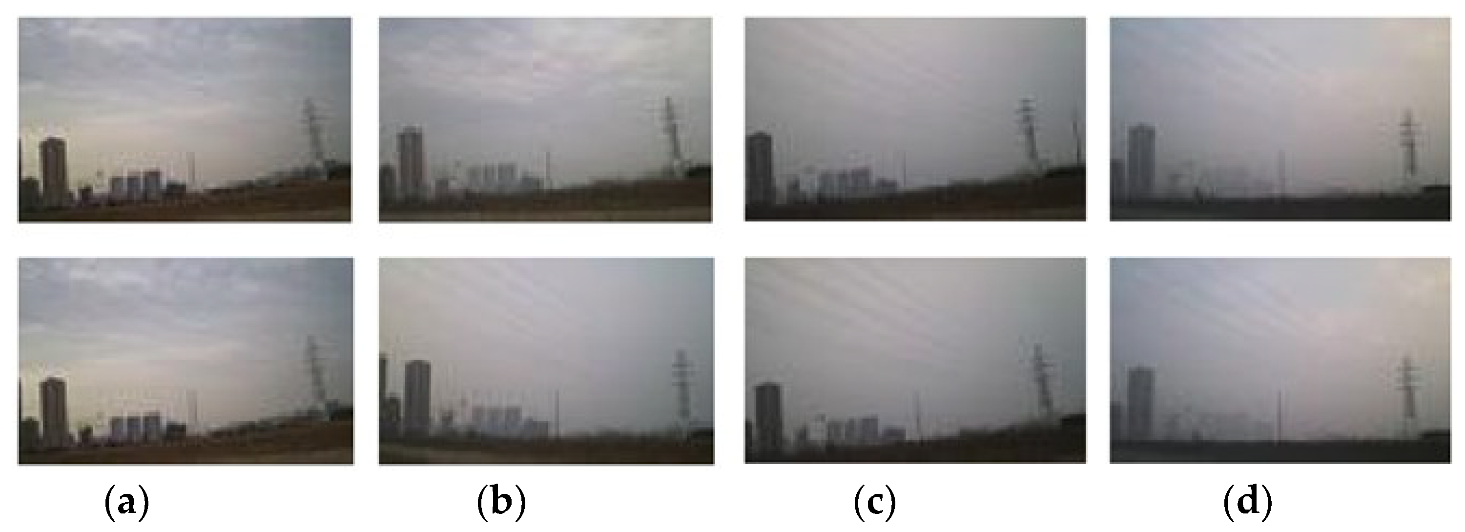
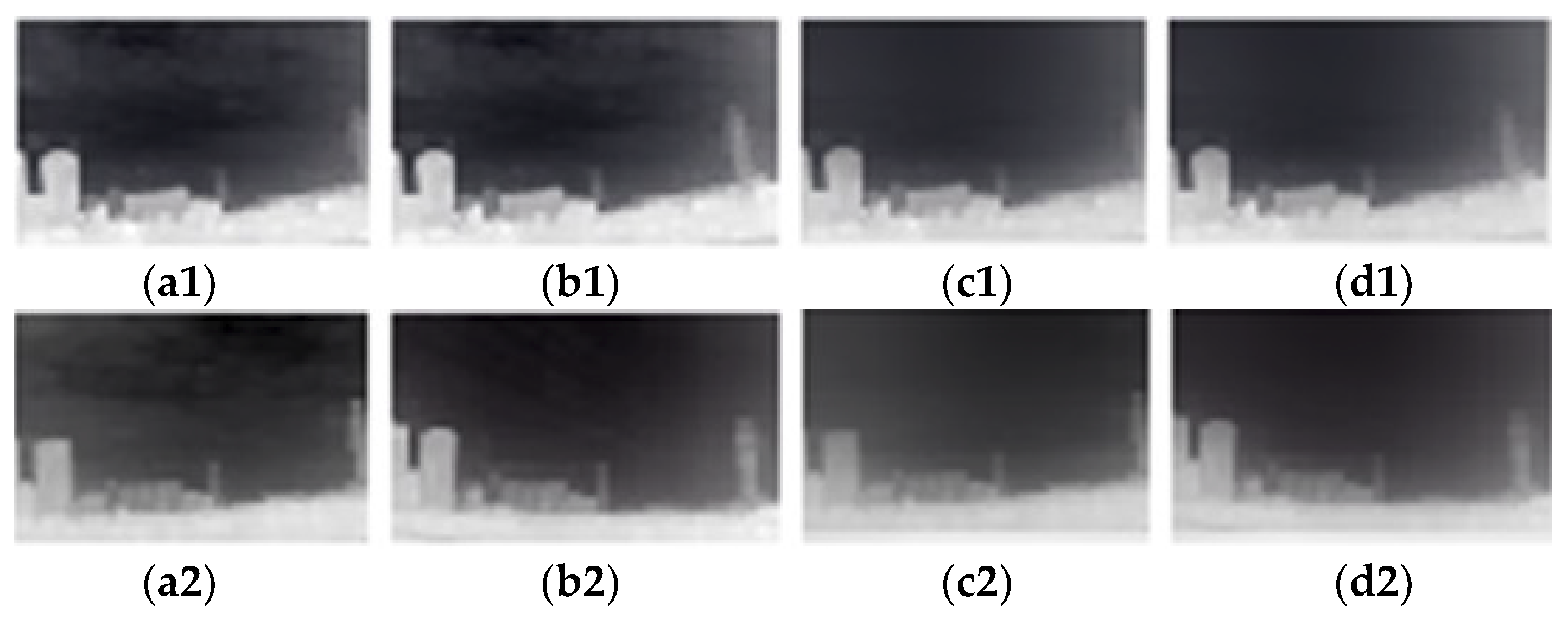
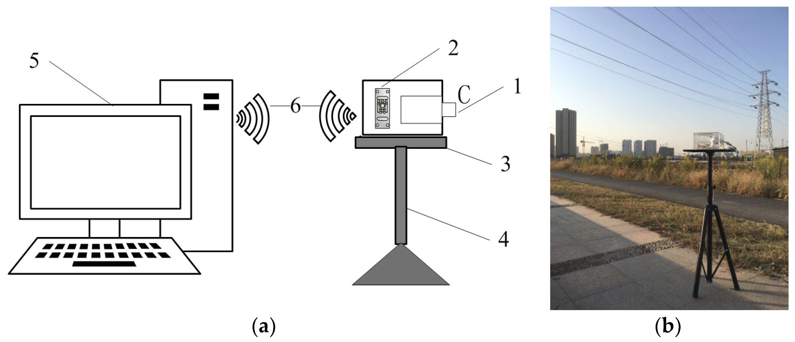
2.1. Materials

The latitude and longitude of the experimental site are longitude 118°70′44′′E and latitude 32°13′29′′N. An image acquisition system is established with a self-made image acquisition device, a router, and a computer, as shown in Figure 1a. The system is used to acquire images and establish an image set for visibility test. The visibility level corresponding to each image is determined, according to the local weather forecast. The image set contains a total of 300 images, which are classified into four levels according to their visibility level: good, mild pollution, moderate pollution, and heavy pollution, with 75 images per level. The field experiment is shown in Figure 1. Some of the acquired images are shown in Figure 2.

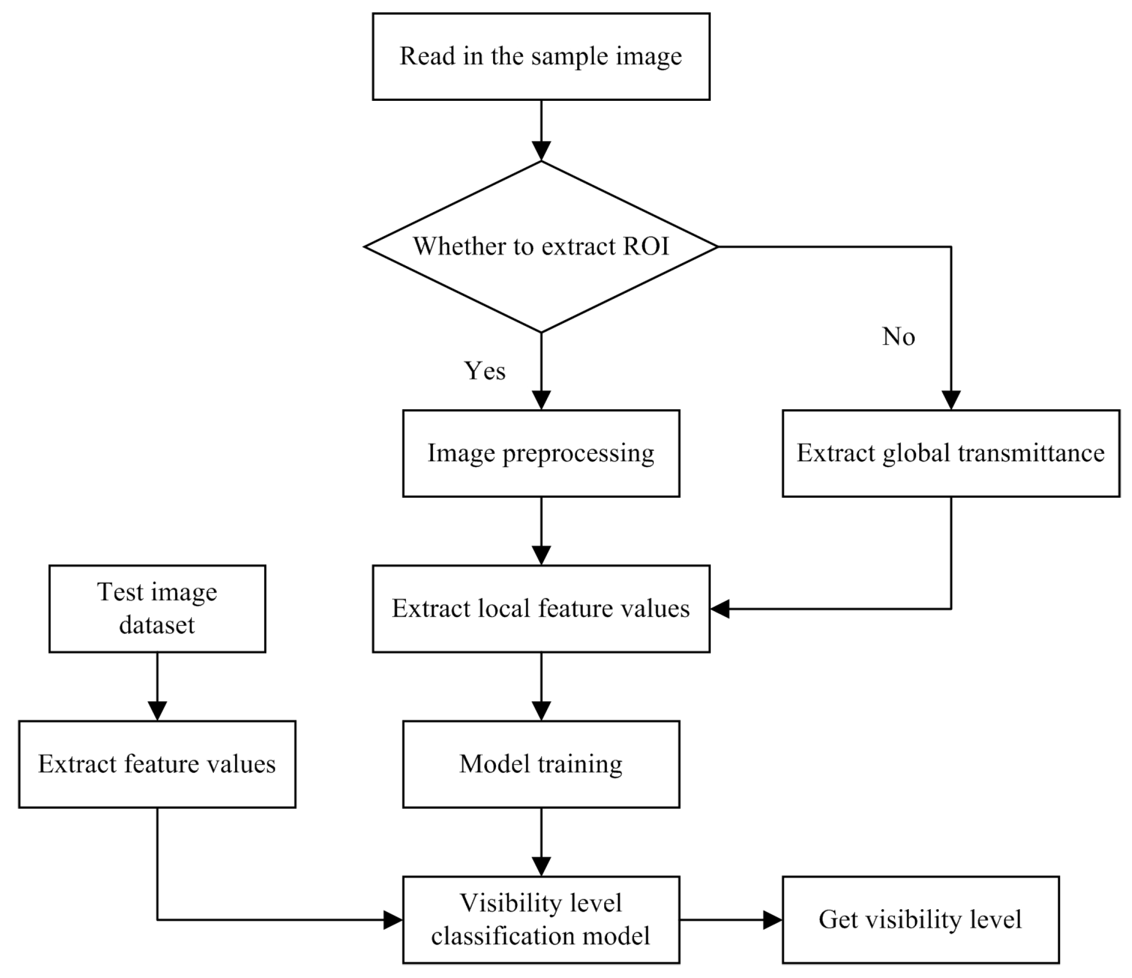
2.2. Visibility Recognition Method

The visibility recognition method based on SVM can be divided into four steps: ROI extraction, image preprocessing, feature value extraction, and model training. The flowchart is shown in Figure 3.

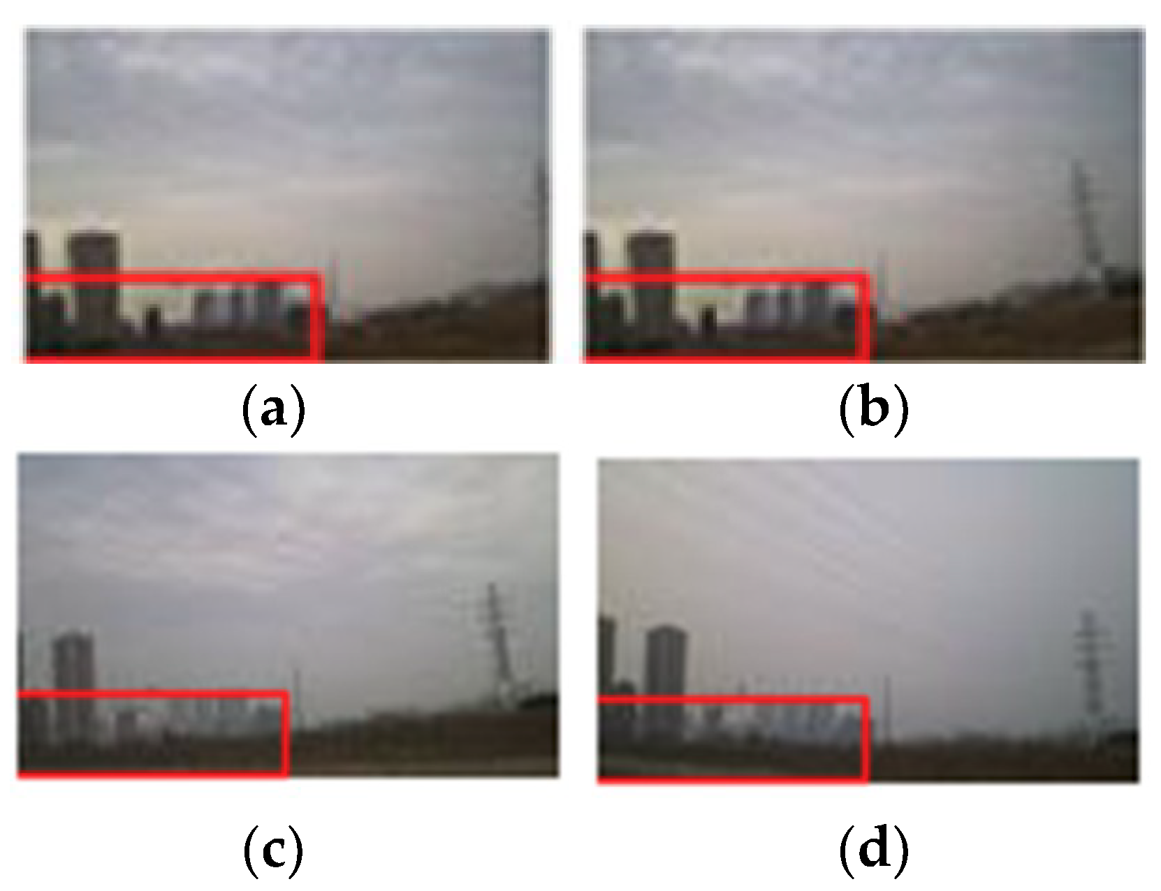
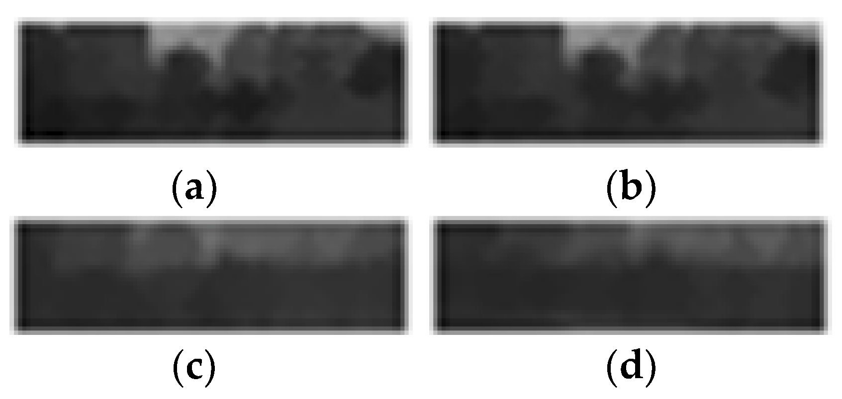
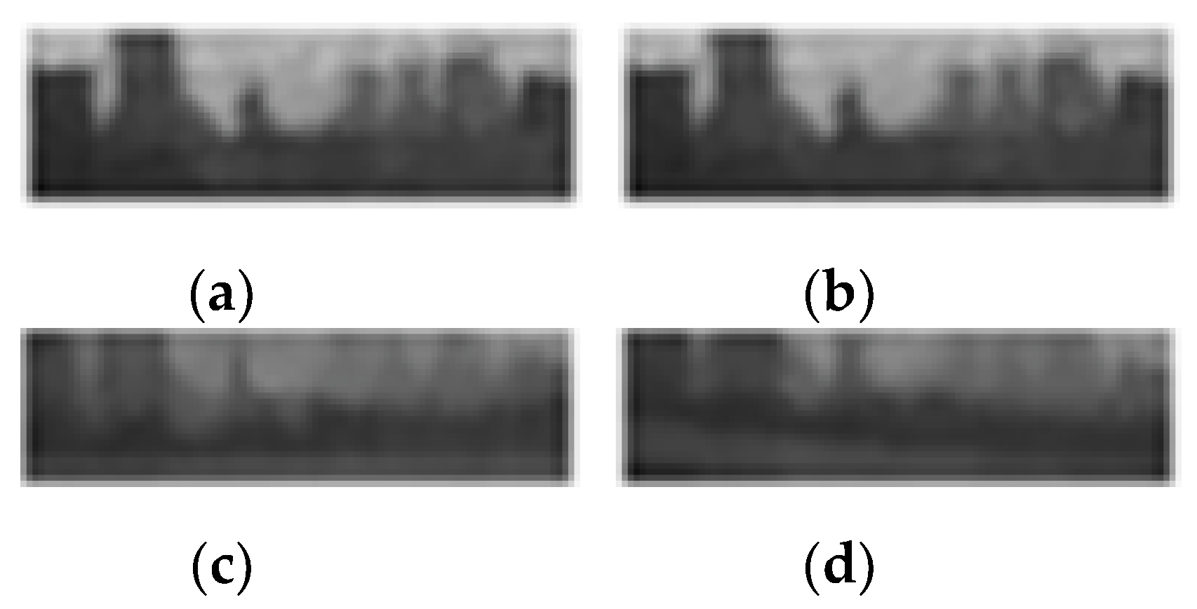
2.2.1. ROI Extraction

In a saliency map, a pixel represents the saliency of a certain point in the input image. In this paper, the ROI extraction is conducted based on the saliency region, where the saliency map is generally introduced through the visual attention model, then the foreground and background information obtained from the visual attention model is integrated, and finally, the image segmentation method is used to finish the ROI extraction [14].

This paper obtains a saliency map in frequency domain [15]. Firstly, Fourier transform is performed to obtain the frequency domain of the image, and to calculate the amplitude spectrum and phase spectrum. Then, the amplitude spectrum is transformed into a logarithmic spectrum. Finally, the logarithmic spectrum is linearly filtered using a linear spatial filter. The difference between the logarithmic spectrum, and the processed amplitude spectrum is defined as the residual spectrum $R\left(f\right)$, as expressed by:

$$R\left(f\right)=log\left(A\left(f\right)\right)-h_n\left(f\right)\times log\left(A\left(f\right)\right)$$

(1)

where f is the Fourier transform spectrum of the image, A(f) is the amplitude spectrum of the image, log(A(f)) is the logarithmic spectrum of the amplitude spectrum, and h_n(f) is the local average filter.

The inverse Fourier transform is performed on the residual spectrum, and the phase spectrum to obtain a saliency value for each point in the image. To get better results, the unprocessed image is linearly filtered using an 8 × 8 Gaussian filter with a mean of 8, and then normalized to obtain the final saliency map S(x):

$$S\left(x\right)=g\left(x\right)\times {\mathrm{F}}^{-1}{\left[exp\left(R\left(f\right)+P\left(f\right)\right)\right]}^2$$

(2)

where g(x) is a Gaussian filter in linear space, P(f) is the phase spectrum of the image, exp is an exponential function, and F⁻¹ is the inverse Fourier transform.

Next, the saliency map is automatically binarized by Otsu’s segmentation algorithm [16]. Then the binary image is divided into a plurality of rectangles with 50 pixels × 15 pixels. The rectangle with the largest number of salient points in the rectangle is selected as the final saliency region, i.e., ROI. The results of the selection are shown in Figure 4.

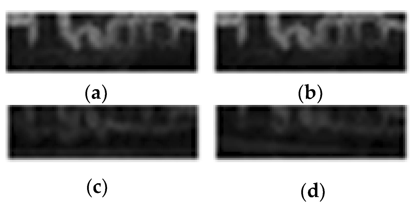
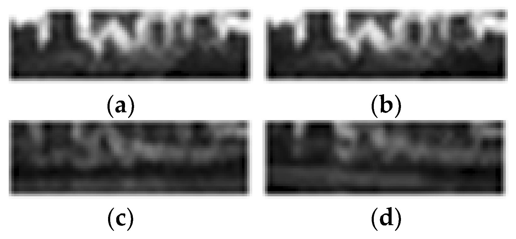
2.2.2. Image Preprocessing

2.2.2.1. Expansion and Erosion

Expansion is the process of merging all background points that are in contact with an object, into the object, eventually causing the boundary to expand outward. Expansion operation can fill the small holes in the image and small concaves at the edges of image, thereby eliminating noise in the target area. Erosion is the dual operation of expansion. Erosion is an operation that eliminates boundary points and that shrinks the boundaries toward the inside of the target area. Small and meaningless objects, as well as noise, can be eliminated by erosion operation.

In this paper, the images after expansion are subtracted from the image after erosion to obtain gradient images. The results of four kinds of air visibility levels are shown in Figure 5, Figure 6 and Figure 7.

2.2.2.2. Linear Contrast Stretch

For the images with lower visibility, their edge features need to be enhanced to improve the matching accuracy. Commonly-used contrast enhancement methods include histogram equalization and contrast stretch. Since contrast enhancement is used to improve the accuracy of feature values extraction, whereas histogram equalization reduces the contrast of useful information, this paper uses linear contrast stretch to enhance edge features [17]. The results of four kinds of air visibility levels are shown in Figure 8.

2.2.3. Extraction of Feature Values

The feature values of the pre-processed image are extracted, including edge features, local contrast features, and global transmittance. The edge features and local contrast features are extracted based on ROI image, while the transmittance features are extracted based a on global image.

2.2.3.1. Calculation of Transmittance

In most non-sky local areas, there are some pixels that always have a very low value in at least one color channel, that is, the minimum value of the intensity of the region is a small number, and the dark channel prior principle [18] indicates that the value usually tends to zero. For any input image J, the dark channel J^dark (x) is defined by:

$$J^{dark}\left(x\right)=\underset{y\in \Omega \left(x\right)}{\min }(\underset{c\in \left\{r,g,b\right\}}{\min }{J}^c\left(y\right))$$

(3)

where Ω(x) is a window centered on pixel x, r, g and b represent the three channels of red, green and blue (RGB) of the color image, c is one of the channels, and J^c(y) is the value of pixel y in channel c, and min indicates the minimum value. The dark channel prior principle satisfies J^dark→0.

For the digital image captured by camera, the optical imaging is mainly formed by two parts: the light reflected by object and the atmospheric light. In computer vision and computer graphics, the commonly used digital foggy imaging model is expressed as:

$$I\left(x\right)=J\left(x\right)t\left(x\right)+\mathrm{A}\left(1-t\left(x\right)\right)$$

(4)

where I(x) is the observed intensity, J(x) is the scene radiance, A is the global atmospheric light, and t(x) is the transmittance feature value needs to be extracted in this paper. According to the dark channel prior principle, and by minimizing Equation (4) twice, the transmittance [19] can be obtained by:

$$t\left(x\right)=1-\underset{c}{\min }\left(\underset{y\in \Omega \left(x\right)}{\min }(\frac{I^c\left(y\right)}{A^c})\right)$$

(5)

where I^c represents the value in channel c of the foggy input image, and $A^c$ represents the value in channel c of the global atmospheric light component.

The above inference assumes that the global atmospheric light component is known. In actual calculations, the value of $A^c$ can be obtained from the foggy image using the dark channel map. The specific steps are as follows:

(1)

Extract the value I of the 0.1% pixels with the largest luminance from the dark channel map.

(2)

Search the maximum value among these values and take it as the global atmospheric light value.

Since the transmittance obtained by this method is too rough, the fast guided filter is employed in this paper to optimize Equation (5). The principle of fast guided filtering is as follows:

(1)

The filtering result at pixel i can be expressed as a weighted average, as expressed by:

$$Q_i={\displaystyle \sum }_j{W}_{i,j}\left(H\right)I_j$$

(6)

where i and j represent the abscissa and ordinate of the image plane, H is the guided image; $I_j$ is the value before filtering, $Q_i$ is the value after filtering, and $W_{ij}$ is a function related to the guided image H. This function is independent of the image p to be processed.

(2)

Assuming that the guided filter is a local linear model in a two-dimensional window between the guided image H and the filtered output Q, which is expressed by:

$$Q_i=a_k{H}_i+b_k\left(\forall \in {\omega }_k\right)$$

(7)

where a and b are the coefficients of the linear function when the center of the window is at k; $Q_i$ is the kernel function related to the transmittance map before filtering; ${\omega }_k$ is the current processing window of image I; $\forall \in {\omega }_k$ indicates that any pixel in the current processing window satisfies Equation (7).

(3)

To minimize the difference between the pre-filtered image J and the filtered image Q, the kernel functions adopted by the coefficients a and b of the fast guided filter are shown by:

$$a_k=\frac{\frac{1}{\left|\omega \right|}{{\displaystyle \sum }}_{i\in {\omega }_k}{H}_i{I}_i-{\mu }_k{\overline{I}}_k}{{\delta }_k{}^2+\epsilon }$$

(8)

$$b_k={\overline{I}}_k-a_k{\mu }_k$$

(9)

where ${\mu }_k$ and ${\delta }_k{}^2$ are is the mean value and variance of the pixel intensity in the current window of the image H, respectively; $\left|\omega \right|$ is the number of pixels in the window; $\overline{I}$ indicates the mean of I values for each pixel in the current window.

The images with more accurate transmittance are obtained by fast guided filtering. The results before and after the fast guided filtering are compared in Figure 9. As can be seen from the figure, part of the noise in the image is removed after the filtering, which makes the image smoother and the transmittance obtained more accurate.

2.2.3.2. Edge Features

Edge features are extremely important information in image processing and computer vision. The gradient is calculated by examining the grayscale change of each pixel in a certain area in an image to find the set of pixels with the greatest brightness change. The edge-detection method determines the edge of an area by using first-order or second-order derivatives. The experimental comparison shows that the Sobel operator has a better ability to detect edges in foggy image. The Sobel operator extracts the edge using the fast convolution function, and the pixels at different positions have different weights. Therefore, this paper uses the Sobel operator for edge detection. The calculated local gradient value is a vector. The absolute value of the calculated gradient is used as the gradient amplitude, and the global average gradient value of the image is used as the gradient feature value, which is defined by:

$$F\left(G_{mean}\right)=\frac{{{\displaystyle \sum }}_i^M{{\displaystyle \sum }}_j^N\left|G_s\left(i,j\right)\right|}{M\times N}$$

(10)

where $F\left(G_{mean}\right)$ is the global average gradient value; M, N indicate the size of the image; $G_s\left(i,j\right)$. is the gradient value of the pixel (i, j) after Sobel operator processing.

2.2.3.3. Extraction of Local Contrast

Another important feature is contrasted feature. Whether an object can be recognized is based on contrast. The definition of contrast in each field is different. The LIP model proposed by Jourlin and Pinoli [20] defines the semi-closed operation on the real interval $[0,M)$. In this model, the contrast of two adjacent pixels (x₁, y₁) and (x₂, y₂) is defined by:

$${\mathrm{C}}_{\left(\left(x1,y1\right),\left(x2,y2\right)\right)}=\frac{M\left|f\left(x1,y1\right)-f\left(x2,y2\right)\right|}{M-min\left(f\left(x1,y1\right),\left(x2,y2\right)\right)}.$$

(11)

where M is taken as 255 in an 8-bit grayscale image, f = M = 255, when the image is all black, f = 0 when the image is all white. In actual image processing, f = 255 when the image is all white, f = 0, when image is all black, so the equation needs to be reversed. Let F = 255—f, bring it into Equation (10), normalize the equation, and we have:

$${\mathrm{C}}_{\left(\left(x1,y1\right),\left(x2,y2\right)\right)}=\frac{\left|F\left(x1,y1\right)-F\left(x2,y2\right)\right|}{max\left(F\left(x1,y1\right),\left(x2,y2\right)\right)}$$

(12)

where ${\mathrm{C}}_{\left(\left(x1,y1\right),\left(x2,y2\right)\right)}$ is the contrast value of the corresponding pixel (x₁, y₁) along the x-axis, and F(x₁, y_1s) and F(x₂, y₂) are the gray values of the corresponding pixels. F(x₂, y₂) is the value of the pixel on the adjacent right side of the pixel (x₁, y₁), and M is the maximum gray value of the image F. Each pixel (x₀, y₀) has eight adjacent pixels, so each pixel has eight contrasts. The contrast feature value of the pixel (x₀, y₀) is defined as:

$$x={\mathrm{maxC}}_{\left(\left(x0,y0\right),\left(x1,y1\right)\right)},\left(x_i,y_i\right)\in V.$$

(13)

where V is a neighborhood pixel set.

The results of the image feature values extracted from a part of the dataset are shown in

Table 1. Image feature extraction results from a part of the dataset according to extraction methods of edge feature, local contrast, and red, green and blue (RGB) channel transmittance.

Levels of Visibility	Edge Features	Eraction of Local Contrast	R Channel Transmittance	G Channel Transmittance	B Channel Transmittance
good air quality	2009.631	0.002457	0.40	0.40	0.43
mild pollution	461.629	0.001429	0.39	0.39	0.40
moderate pollution	645.9079	0.001429	0.40	0.38	0.39
heavy pollution	730.431	0.002457	0.34	0.33	0.35
good air quality	2002.341	0.002457	0.40	0.40	0.42
mild pollution	460.9177	0.001314	0.37	0.36	0.37
moderate pollution	708.7448	0.001714	0.36	0.35	0.35
heavy pollution	731.2064	0.0024	0.37	0.34	0.33

according to the above methods. From Table 1, the edge feature values and local contrast feature values of the images are significantly distinguished between different air visibility levels, while the transmittance values of the RGB channels are slightly different. The transmittance values of RGB in the same image are almost the same.

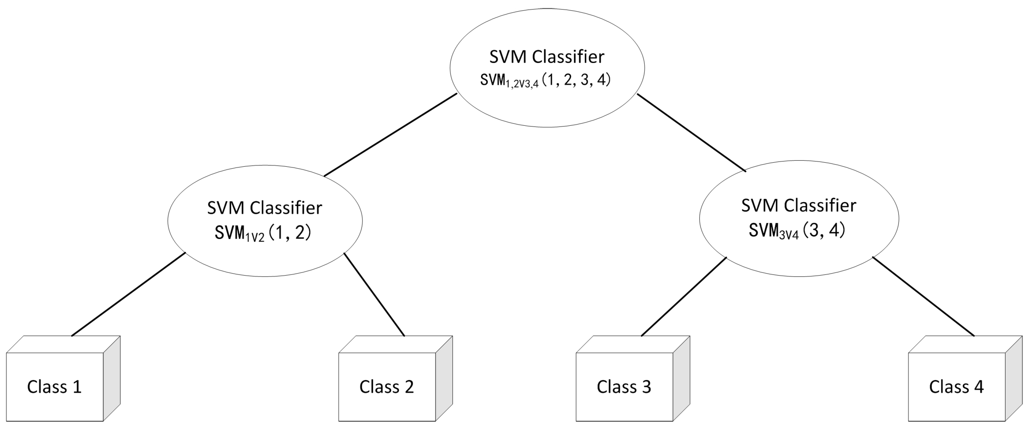
2.2.4. Multi-Classification Model Based on Binary Tree SVM

After extracting the features of different images, the visibility recognition model is established through SVM training. Support vector machine (SVM) is a classifier based on structural risk minimization. By solving the quadratic programming problem, the best hyperplane that can divide the data into two categories can be determined [21,22].

SVM is originally proposed for solving the binary-classification problem. For the multi-classification problem [23], we can refer to binary classification and classify all categories into two sub-categories, which are then classified into two secondary sub-categories. The process continues until the entire individual category is obtained. So, a multi-classifier can be constructed to achieve multi-classification SVM using a certain combination scheme. At present, the multi-classification SVMs are mainly constructed by a one-to-one method and a one-to-many method. The one-to-one method has inseparable regions in classification, and the one-to-many method has an unsatisfying performance. Therefore, faced with the shortcomings of these two methods, this paper proposes a multi-classification SVM based on binary tree [24,25]. A schematic diagram of constructing a classifier is shown in Figure 10.

In this paper, air visibility is classified into four levels: good air quality, mild pollution, moderate pollution, and heavy pollution, which are represented by Class 1, Class 2, Class 3, and Class 4, respectively. So, a 2-layer optimal binary tree is constructed. The SVM_1,2V3,4 on the first layer mainly recognizes Class 1, Class 2, Class 3, and Class 4, and the SVMs on the second layer are SVM_1V2 and SVM_3V4, where SVM_1V2 recognizes Class 1 and Class 2, while SVM_3V4 recognizes Class 3 and Class 4. The categories under each SVM are selected according to the maximum threshold interval. The maximum branch interval under each node can effectively reduce the error of classification and recognition, and avoid the problem of the downward accumulation of errors, thus obtaining the optimal binary tree with the highest classification and recognition accuracy. The process of recognizing the air visibility level by the 2-layer optimal binary tree SVM is as follows:

Step 1

Extract the feature vectors of the images of four visibility levels. Firstly, start from the root node 1, calculate the SVM (serial number), and judge the next destination according to the output value. If the visibility level of the image is Class 1 or Class 2, then go to the left leaf node (serial number) of layer 2, and if the visibility level belongs to Class 3 or Class 4, then go to the right leaf node (serial number) of layer 2.

Step 2

Go to the left leaf node, calculate the classifier (serial number). If the result of this air visibility level is positive, it belongs to Class 1, otherwise, it belongs to Class 2.

Step 3

Go to the right leaf node, calculate the classifier (serial number). If the result of this air visibility level is positive, it belongs to Class 3, otherwise, it belongs to Class 4.

3. Results and Discussion

3.1. Results of Visibility Level Recognition Based on the Proposed Method

In the experiment, 50 images were randomly selected from each set of 75 images, and a total of 200 images were used as training samples. The remaining 25 images of each visibility levels were used as test samples, with a total of 100 test samples. The model based on optimal binary tree SVM was constructed by MATLAB software to recognize and classify the images. In this model, the inner product kernel function of each optimal binary tree classifier used the radial basis kernel function $\mathrm{k}\left(x_i,x_j\right)=exp\left(-\frac{{\left|x_i-x_j\right|}^2}{2{\sigma }^2}\right)$. The kernel width σ and the error penalty parameter C of the kernel function were adjusted by the cross-validation of the sample set at each node to obtain the optimal parameters.

The classification and recognition results are shown in

Table 2. Test results of air visibility classification by four kinds of visibility levels.

Classifier Recognition Accuracy	Levels of Visibility
	Good Air Quality	Heavy Pollution	Mild Pollution	Moderate Pollution
Classifier SVM1,2V3,4 recognition accuracy (%)	96.00	100	96.00	92.00
Classifier SVM1V2 recognition accuracy (%)	92.00	100	NA 1	NA
Classifier SVM3V4 recognition accuracy (%)	NA	NA	92.00	88.00
Single level recognition accuracy (%)	92.00	100	92.00	88.00
Average recognition accuracy (%)	93.00

¹ NA represents no value.

. In the model of the 2-layer optimal binary tree SVM, the root node classifier SVM_1,2V3,4 on the first layer achieved recognition accuracies of 96.00%, 100%, 96.00%, and 92.00% for good air quality and heavy pollution (Class 1, Class 2), mild pollution, and moderate pollution (Class 3, Class 4), respectively. The leaf node classifier SVM_1V2 on the second layer achieved recognition accuracies of 92.00% and 100% for good air quality and heavy pollution, respectively. The leaf node classifier SVM_3V4 achieved the recognition accuracies of 92.00% and 88.00% for mild pollution and moderate pollution, respectively. In summary, the recognition accuracies of air visibility level by the proposed method were 92.00%, 92.00%, 88.00%, and 100.00% for good air quality, mild pollution, moderate pollution, and heavy pollution, respectively, with an average recognition accuracy of 93.00%. The experimental results showed that the proposed model based on the optimal binary tree SVM achieved satisfactory recognition accuracy for the air visibility level.

3.2. Comparison between the Proposed Method and Traditional Methods

In order to further verify that the proposed method performs better than the traditional SVM methods, a comparison was made between the proposed method and one-to-one SVM method as well as one-to-many SVM method. Both the two traditional methods used the same radial basis kernel function as the method proposed in this paper. The one-to-one SVM had a total of four classifiers, and the one-to-many SVM had a total of four classifiers. In this experiment, both the training set and test set were the same as those in Section 3.1, that is, 200 images of four visibility levels were used as training set, and 100 images of four visibility levels were used as the test set.

The training time of the three different methods is shown in Table 2. As can be seen from the table, the training time of the one-to-one SVM method, the one-to-many SVM method, and the proposed method was 6.5 s, 6.7 s, and 6.0 s, respectively, that is, the training time of the proposed method was shorter than that of the other two methods. The reason for this is that the proposed method adopted the structure of the optimal binary tree, which reduced the number of required SVM classifiers, thus shortening the time required for training samples.

The recognition accuracy of air visibility level using the three different methods are shown in

Table 3. The results of training time and recognition rate by using three methods: one-to-one SVM, one-to-many SVM, and the proposed method.

Method	Training Time (Unit: s)	Recognition Rate (%)
one-to-one SVM	6.5	88.00
one-to-many SVM	6.7	90.00
proposed method	6.0	93.00

. The recognition accuracy of the air visibility level by one-to-one SVM, one-to-many SVM, and the proposed method were 88.00%, 90.00%, and 93.00%, respectively. Therefore, it can be seen from the recognition accuracy that the proposed method had higher recognition accuracy than the other two traditional SVM methods.

4. Conclusions

(1)

Using the saliency map acquired in the frequency domain of the image, the ROI extracted by the saliency region is salient in the image, which can fully reflect the features of the image, so that the feature values extracted in the ROI can be easily distinguished.

(2)

The transmittance feature values extracted using the dark channel prior principle have three channels of R, G, and B, which can reflect slight differences between different air visibility levels. In addition, rapid guided filtering is employed to optimize the extraction of the transmittance, so that the feature value of transmittance is more distinguishable for different air visibility levels.

(3)

This paper constructs a model for recognizing air visibility level based on the optimal binary tree SVM. After the calculation of the optimal binary tree and three SVMs, four air visibility levels can be recognized. Combined with the cross-validation method, the recognition accuracy of good air quality, mild pollution, moderate pollution, and heavy pollution are 92.00%, 92.00%, 88.00%, and 100.00%, with an average recognition accuracy of 93.00%. Therefore, the method is able to recognize four air visibility levels in a relatively accurate way.

References

1. Tai, H.; Zhuang, Z.; Jiang, L.; Sun, D. Visibility measurement in an atmospheric environment simulation chamber. Curr. Opt. Photonics 2017, 1, 186–195. [Google Scholar]
2. Kim, K.W. The comparison of visibility measurement between image-based visual range, human eye-based visual range, and meteorological optical range. Atmos. Environ. 2018, 190, 74–86. [Google Scholar] [CrossRef]
3. García, J.A.; Rodriguez-Sánchez, R.; Fdez-Valdivia, J.; Martinez-Baena, J. Information visibility using transmission methods. Pattern Recognit. Lett. 2010, 31, 609–618. [Google Scholar] [CrossRef]
4. Kim, K.S.; Kang, S.Y.; Kim, W.S.; Cho, H.S.; Park, C.K.; Lee, D.Y.; Kim, G.A.; Park, S.Y.; Lim, H.W.; Lee, H.W.; et al. Improvement of radiographic visibility using an image restoration method based on a simple radiographic scattering model for x-ray nondestructive testing. NDT E Int. 2018, 98, 117–122. [Google Scholar] [CrossRef]
5. Gultepe, I.; Müller, M.D.; Boybeyi, Z. A New Visibility Parameterization for Warm-Fog Applications in Numerical Weather Prediction Models. J. Appl. Meteorol. Clim. 2006, 45, 1469–1480. [Google Scholar] [CrossRef]
6. He, X.; Zhao, J. Multiple lyapunov functions with blending for inducedl2-norm control of switched lpv systems and its application to an f-16 aircraft model. Asian J. Control 2014, 16, 149–161. [Google Scholar] [CrossRef]
7. Yanju, L.; Hongmei, L.; Jianhui, S. Research of highway visibility detection based on surf feature point matching. J. Shenyang Ligong Univ. 2017, 36, 72–77. [Google Scholar]
8. Min, X.; Hongying, Z.; Yadong, W. Image visibility detection algorithm based on scene depth for fogging environment. Process Autom. Instrum. 2017, 38, 89–94. [Google Scholar]
9. Xi, X.; Xu-Cheng, Y.; Yan, L.; Hong-Wei, H.; Xiao-Zhong, C. Visibility measurement with image understanding. Intern. J. Pattern Recognit. Artif. Intell. 2013, 26, 543–551. [Google Scholar]
10. Suárez Sánchez, A.; García Nieto, P.J.; Riesgo Fernández, P.; del Coz Díaz, J.J.; Iglesias-Rodríguez, F.J. Application of an svm-based regression model to the air quality study at local scale in the avilés urban area (spain). Math. Comput. Model. 2011, 54, 1453–1466. [Google Scholar] [CrossRef]
11. Bronte, S.; Bergasa, L.M.; Alcantarilla, P.F. Fog detection system based on computer vision. In Proceedings of the 12th International IEEE Conference on Intelligent Transportation Systems, St. Louis, MO, USA, 4–7 October 2009. [Google Scholar]
12. Singh, K.P.; Gupta, S.; Rai, P. Identifying pollution sources and predicting urban air quality using ensemble learning methods. Atmos. Environ. 2013, 80, 426–437. [Google Scholar] [CrossRef]
13. Feng, X.; Li, Q.; Zhu, Y.; Hou, J.; Jin, L.; Wang, J. Artificial neural networks forecasting of PM2.5 pollution using air mass trajectory based geographic model and wavelet transformation. Atmos. Environ. 2015, 107, 118–128. [Google Scholar] [CrossRef]
14. Simu, S.; Lal, S.; Nagarsekar, P.; Naik, A. Fully automatic roi extraction and edge-based segmentation of radius and ulna bones from hand radiographs. Biocybern. Biomed. Eng. 2017, 37, 718–732. [Google Scholar] [CrossRef]
15. Hou, X.; Zhang, L. Saliency detection: A spectral residual approach. In Proceedings of the IEEE Computer Society Conference on Computer Vision and Pattern Recognition, Minneapolis, MN, USA, 17–22 June 2007; pp. 1–8. [Google Scholar]
16. Otsu, N. A Threshold Selection Method from Gray-Level Histograms. IEEE Trans. Syst. Man Cybern. 1979, 9, 62–66. [Google Scholar] [CrossRef]
17. Turner, D.; Lucieer, A.; Malenovský, Z.; King, D.; Robinson, S. Spatial co-registration of ultra-high resolution visible, multispectral and thermal images acquired with a micro-uav over antarctic moss beds. Remote Sens. 2014, 6, 4003–4024. [Google Scholar] [CrossRef]
18. Wang, J.-B.; He, N.; Zhang, L.-L.; Lu, K. Single image dehazing with a physical model and dark channel prior. Neurocomputing 2015, 149, 718–728. [Google Scholar] [CrossRef]
19. Ling, Z.; Li, S.; Wang, Y.; Lu, X. Adaptive transmission compensation via human visual system for robust single image dehazing. Vis. Comput. 2016, 32, 653–662. [Google Scholar] [CrossRef]
20. Jourlin, M.; Breugnot, J.; Itthirad, F.; Bouabdellah, M.; Closs, B. Logarithmic image processing for color images. Adv. Imaging Electron Phys. 2011, 168, 65–107. [Google Scholar]
21. Deshpande, A.; Tadse, S.K. Design approach for content-based image retrieval using gabor-zernike features. Int. J. Eng. Sci. Technol. 2012, 3, 42–46. [Google Scholar]
22. An, Y.; Ding, S.; Shi, S.; Li, J. Discrete space reinforcement learning algorithm based on support vector machine classification. Pattern Recognit. Lett. 2018, 111, 30–35. [Google Scholar] [CrossRef]
23. Tang, F.; Adam, L.; Si, B. Group feature selection with multiclass support vector machine. Neurocomputing 2018, 317, 42–49. [Google Scholar] [CrossRef]
24. Manikandan, J.; Venkataramani, B. Study and evaluation of a multi-class svm classifier using diminishing learning technique. Neurocomputing 2010, 73, 1676–1685. [Google Scholar] [CrossRef]
25. Qin, G.; Huang, X.; Chen, Y. Nested one-to-one symmetric classification method on a fuzzy SVM for moving vehicles. Symmetry 2017, 9, 48. [Google Scholar] [CrossRef]
Figure 1. Image acquisition system and the field test. (a) Air visibility image acquisition system with 1. camera, 2. mainboard, 3. tray, 4. tripod, 5. computer, 6. Wi-Fi connection; (b) The picture of the field experiment site.
Atmosphere 09 00481 g001
Figure 2. Some of the acquired images of air visibility: (a) good air quality; (b) mild pollution; (c) moderate pollution; (d) heavy pollution.
Atmosphere 09 00481 g002
Figure 3. The flowchart of the visibility recognition method based on support vector machine.
Atmosphere 09 00481 g003
Figure 4. The results of the region of interest (ROI) selection by a plurality of rectangles with 50 × 15 pixels: (a) good air quality; (b) mild pollution; (c) moderate pollution; (d) heavy pollution.
Atmosphere 09 00481 g004
Figure 5. The ROI images after expansion are obtained from (a) good air quality; (b) mild pollution; (c) moderate pollution; (d) heavy pollution.
Atmosphere 09 00481 g005
Figure 6. The ROI images after erosion are obtained from (a) good air quality; (b) mild pollution; (c) moderate pollution; (d) heavy pollution.
Atmosphere 09 00481 g006
Figure 7. The gradient images after expansion are subtracted from the images after erosion of (a) good air quality; (b) mild pollution; (c) moderate pollution; (d) heavy pollution.
Atmosphere 09 00481 g007
Figure 8. The edge features of the ROI images are enhanced by using linear contrast stretch from (a) good air quality; (b) mild pollution; (c) moderate pollution; (d) heavy pollution.
Atmosphere 09 00481 g008
Figure 9. The results before and after the fast guided filtering are compared. (a1, b1, c1, d1) Before the fast guided filtering; (a2, b2, c2, d2) After the fast guided filtering. (a1, a2) Good air quality; (b1, b2) Mild pollution; (c1, c2) Moderate pollution; (d1, d2) Heavy pollution.
Atmosphere 09 00481 g009
Figure 10. A schematic diagram of constructing a classifier based on optimal binary tree support vector machine.
Atmosphere 09 00481 g010