1. Introduction
There are two methods that are widely used to represent clouds and precipitation in numerical weather and climate models: bulk and bin microphysics schemes. Usually, bulk microphysics schemes parameterize size distributions of cloud particles using only a few parameters, and calculate microphysical processes by integrating analytic functions. For example, currently most widely used bulk microphysics schemes adopt a kind of gamma distribution with two independent variables (number concentration and mixing ratio) to express drop size distributions, and present the condensational growth rate of drops as a function of the two variables by integrating or approximating the vapor diffusion equation. This method has obvious drawbacks; any analytic function with a few independent variables cannot express arbitrary size distribution shapes. In contrast to bulk microphysics schemes, bin microphysics schemes explicitly express the distributions by dividing cloud particles into a few tens to hundreds of bins and evaluate microphysical processes of the particles in each bin. While bin microphysics schemes are believed to be useful to investigate the evolution of size distributions of particles in clouds, bulk microphysics schemes are widely used in operational weather forecasting, owing to their much lower computational cost than bin microphysics schemes.
Since Ogura and Takahashi [
1] and Soong [
2] developed bin microphysics schemes to represent cloud microphysical processes in numerical models, there has been a growing body of studies that develops and utilizes bin microphysics schemes to better understand clouds and precipitation [
3,
4,
5,
6,
7,
8,
9,
10,
11,
12]. Previous studies have reported that results obtained using bin microphysics schemes are generally closer to observations than those obtained using bulk microphysics schemes (e.g., mesoscale convection, [
3,
4]; mixed-phase cloud system, [
5,
6]; tropical cyclone, [
7]). In addition, some studies have utilized bin microphysics schemes as a benchmark for evaluating or developing bulk microphysics schemes [
13,
14,
15,
16]. Khain et al. [
17] provided a comprehensive comparison between bin and bulk microphysics schemes.
While many of the studies that compare bin and bulk microphysics schemes have focused on comparisons in idealized atmospheric conditions [
18], a few studies have dealt with real cases. Fan et al. [
6] compared the results of a bin microphysics scheme [
19] to those of a double-moment bulk microphysics scheme [
20] in simulating two precipitation cases that occurred in southern China, and examined aerosol effects on the precipitation cases. That study showed that the bin microphysics scheme better simulates deep convective clouds than the bulk microphysics scheme and that the opposite reaction to an increase in aerosol loading is a key mechanism to the differences. Iguchi et al. [
5] compared the results of another bin microphysics scheme [
9] to those of a single-moment bulk microphysics scheme [
21,
22] in simulating three precipitation cases, and showed that the bin microphysics scheme agrees better with observations than the bulk microphysics scheme. Iguchi et al. [
5] suggested the fall velocity of hydrometeors as a key component.
Previous studies that focused on comparisons between bin and bulk microphysics schemes in simulating real cases have tended to choose just one bulk microphysics scheme for comparison, making it somewhat difficult to distinguish differences originating from the choice of a specific scheme and those originating from generic differences between bin and bulk microphysics schemes. Therefore, in this study, several double-moment bulk microphysics schemes are chosen and compared to one bin microphysics scheme. In addition, while previous studies have tended to focus on the expression of particle size distributions, this study investigates whether differences in the results of bin and bulk microphysics schemes can be caused by more appropriate representations on microphysical processes in the bin microphysics scheme. A plausible factor that partially explains differences in simulated surface precipitation is presented, and reliability of the factor is investigated with an additional simulation. The numerical model used in this study, experimental setup, and the selected case are described in
Section 2. Simulation results are presented and discussed in
Section 3 and
Section 4. A summary and conclusions are provided in
Section 5.
2. Model Description, Experimental Setup, and Case Description
The Weather Research and Forecasting (WRF) model v3.7.1 [
23] is used for this study. The bin microphysics scheme of the Hebrew University Cloud Model is implemented in the WRF model [
9,
12,
24]. This scheme evaluates nucleation, vapor diffusion processes (condensation, evaporation, deposition, and sublimation), collision, breakup, freezing, melting, ice crystal multiplication, and sedimentation. Seven hydrometeor types are considered: liquid drop, three ice crystals (column, plate, and dendrite), snow, graupel, and hail. A simplified version of this bin microphysics scheme that deals with warm microphysical processes only has also been used in combination with the WRF model to simulate idealized shallow convective clouds [
25]. The spatiotemporal evolution of particle size distribution of each hydrometeor is evaluated by predicting number concentrations at 43 mass doubling bins, in which the ratio of masses between two adjacent bins is two. In addition to the number concentrations, liquid water fractions at mass grid points of snow, graupel, and hail are predicted to incorporate the gradual melting of large ice particles in the scheme. Rimed fractions of snow are also predicted to update the density and terminal velocity of snow particles. Note that the bin microphysics scheme used in this study is somewhat different from the publicly available version [
12], in which the number of bins for each hydrometeor and aerosol is 33 and some microphysical processes (e.g., gradual melting), as well as liquid water fractions of large ice particles and rimed fractions of snow particles, are not predicted.
The number concentration of aerosols is calculated using 43 mass doubling bins, in which the maximum radius of aerosols is 2 μm. Aerosols are activated into liquid drops if their radii are larger than the critical radius determined by environmental supersaturation according to the Köhler theory. The radius of newly activated droplets is determined to be the larger of the smallest radius in the mass bin grid and five times the dry aerosol radius, to consider the effects of giant aerosols [
26]. Ice crystals form by stochastic freezing of drops [
27], or by deposition and condensation-freezing nucleation [
28], or by ice crystal multiplication [
29]. The mass of newly formed ice crystals is either that of frozen drop (via stochastic freezing) or the smallest mass in the mass bin grid (via nucleation or multiplication). Compared to Lee and Baik [
24], the scheme is further improved by including the breakup of large snow particles following Khain et al. [
9]. Turbulence-induced collision enhancement is not included.
For bulk microphysics schemes, the WRF Double-Moment 6-class (WDM6) scheme [
30], Milbrandt scheme [
31], Thompson–Eidhammer (or Thompson aerosol-aware) scheme [
32], and National Severe Storms Laboratory (NSSL) scheme [
33] are used. All of the selected bulk microphysics schemes predict cloud droplet number concentration and raindrop number concentration; in other words, they are double-moment for liquid drops. Note that although all of the bulk microphysics schemes are double-moment for liquid drops, there are noticeable differences among them. For example, the WDM6 scheme is single-moment for all ice particles [
34], and the Thompson–Eidhammer scheme for snow and graupel. The Milbrandt scheme does not consider aerosol number concentration in the drop activation process and predicts the number of nucleated droplets using a hardwired method [
35]. The Milbrandt and NSSL schemes consider explicit hail, whereas the WDM6 and Thompson–Eidhammer schemes predict graupel as the only rimed ice particle.
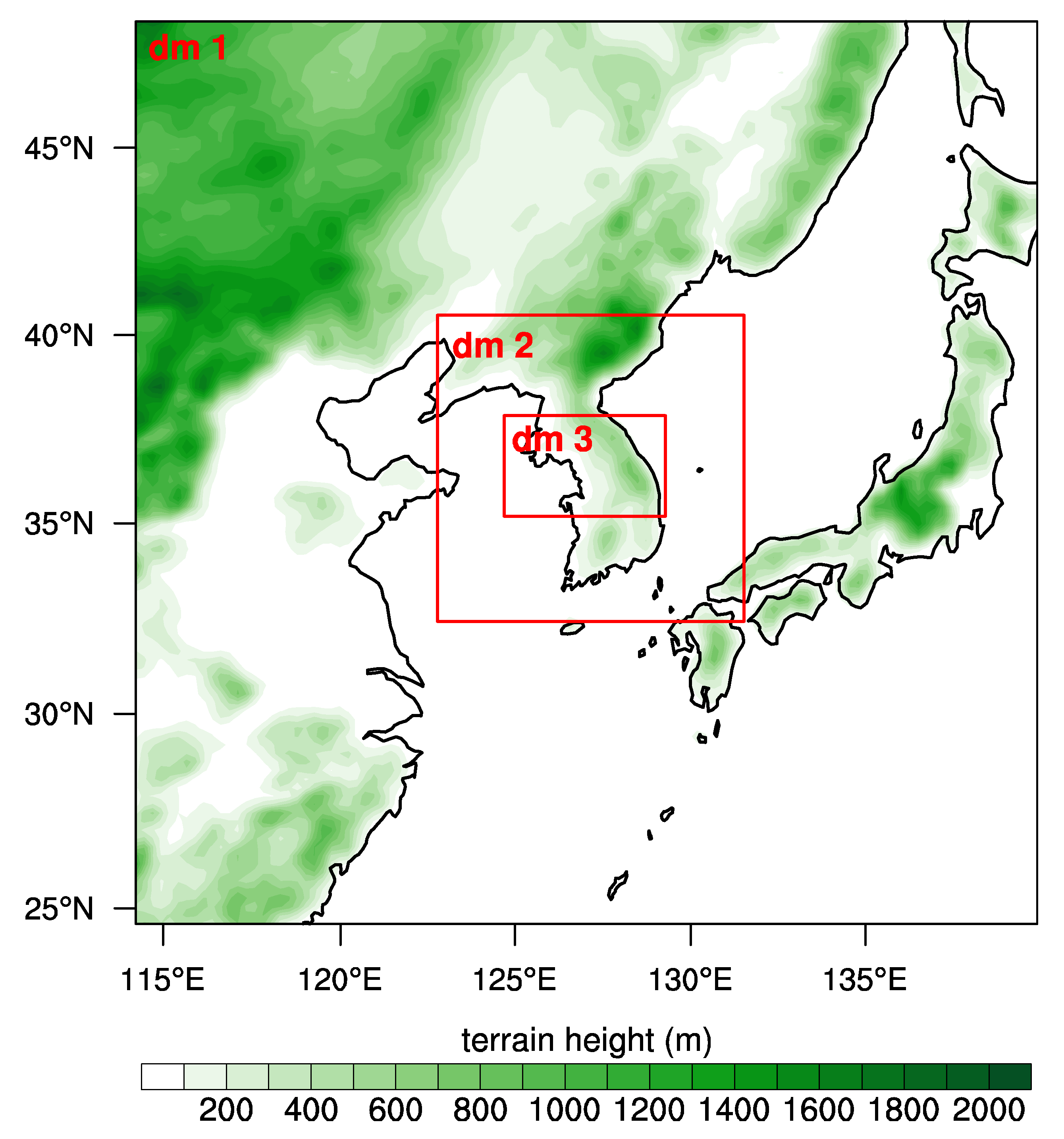
Three one-way nested domains are set for the model calculation. The numerical model setup including domain configuration is the same as in Lee and Baik [
24], which is summarized and depicted in
Figure 1,
Table 1 and
Table 2. The subgrid-scale cumulus scheme is applied only to domain 1. The model top is at 50 hPa (approximately 20 km). The domain is vertically divided into 33 layers. The vertical grid size is finest at the surface with ~30 m, and ~800 m in the free atmosphere. National Centers for Environmental Prediction (NCEP) Final (FNL) analysis data [
36] that have a spatial resolution of 1° × 1° and a temporal resolution of 6 hr are used for the initial and boundary conditions of the outermost domain. In all simulations, the aerosol number concentration is set to be approximately 700 cm
−3, which is similar to the hardwired value assumed in the polluted case of the Milbrandt scheme and supported by observations of long-term variations of aerosol concentration in and around the Korean Peninsula [
37]. In the bin microphysics scheme, the initial aerosol size distribution is set to follow the Twomey equation [
38], which is expressed as:
where
ra is the radius of aerosol,
N0 is the number concentration of activated aerosols at supersaturation of 1%,
k is a constant that controls the slope of aerosol size distribution, and
A and
B are coefficients related to the curvature and solute effects, respectively [
24].
A precipitation case that occurred on 21 September 2010 in the central region of the Korean Peninsula (roughly covered by domain 3 in
Figure 1) is simulated. The maximum hourly precipitation rate and the maximum daily accumulated precipitation amount in this case reached approximately 100 mm hr
−1 and 300 mm, respectively. In this case, the relatively cold and dry Siberian high was on the northwest side of the Korean Peninsula, and the relatively warm and moist western Pacific subtropical high was on the southeast side of the Korean Peninsula. A large amount of low-level moisture was supplied to the central Korean Peninsula by westerly winds along the edge of the western Pacific subtropical high. Precipitation occurred at a stationary front induced by the convergence of these two different air masses over the Korean Peninsula while thermodynamic instability (such as convective available potential energy) was low throughout the precipitation period. These features are common characteristics in heavy precipitation cases in the Korean Peninsula; hence, this case could be a representative of typical heavy precipitation in the Korean Peninsula. A detailed description of this case is given in Jung and Lee [
44] and Lee and Baik [
24]. The model is integrated for 24 hr from 21:00 LST (local standard time, UTC+09:00) 20 September. The first 6 hr is excluded from analysis considering the spin-up time of the model, and the remaining 18-hr data are used for analysis.
3. Comparison of Simulations to Observations
In this section, a simple comparison of simulation results to observations is presented. Because evaluations of the simulation results obtained using the bin microphysics scheme against observations are given in Lee and Baik [
24] in more detail and the main purpose of this study is to compare bin microphysics scheme to bulk microphysics schemes, only a simple description focusing on performance comparison is given in this study.
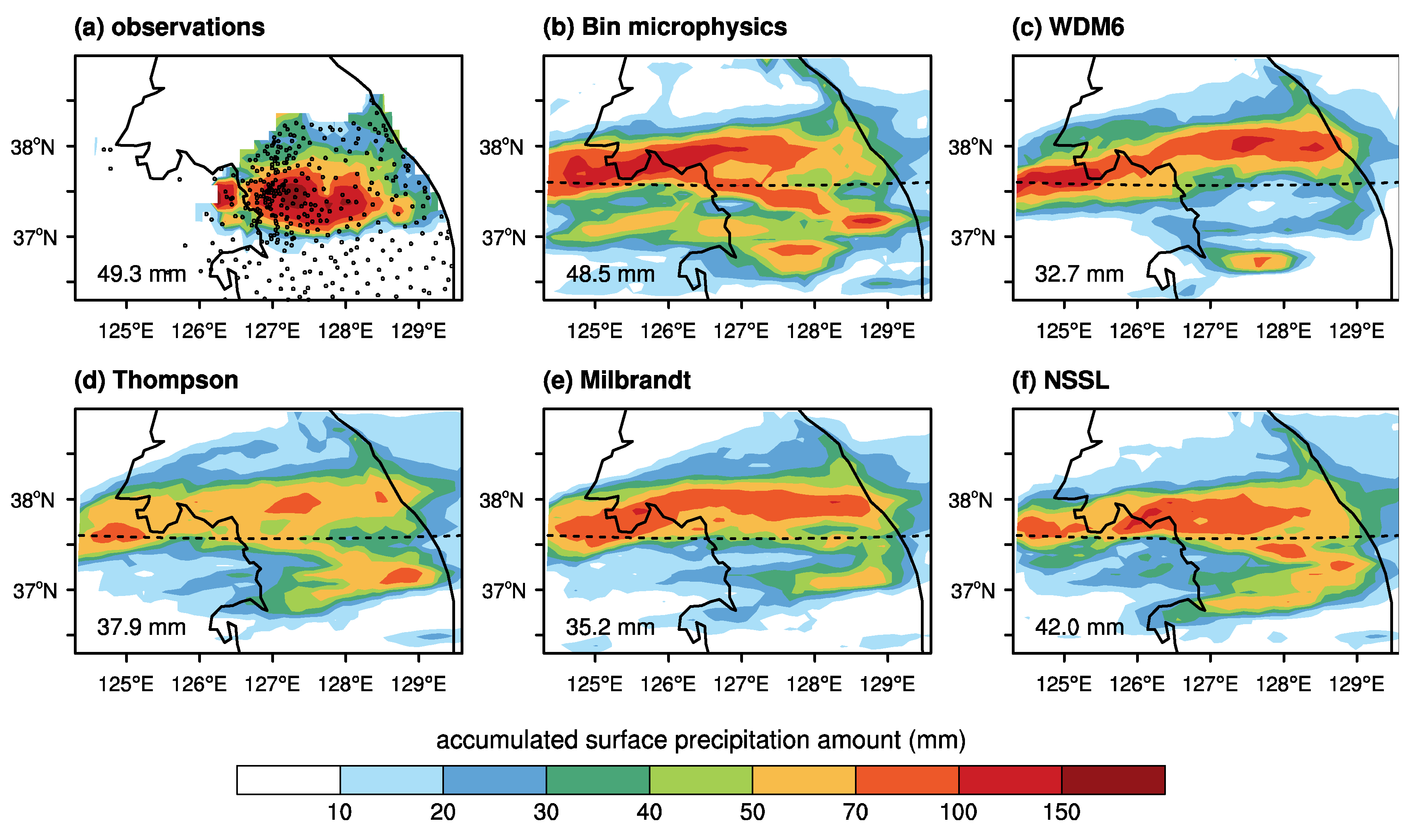
Figure 2 shows the 18-hr accumulated surface precipitation amounts observed by automatic weather systems (AWSs) and simulated by the model with different microphysics schemes. The number of AWSs is 346, whose locations are marked in
Figure 2a. Surface precipitation amounts accumulated for every 15-min interval at each AWS are used. All of the simulations show two distinctly different precipitation bands: one north of ~37.6° N (the northern precipitation hereafter) and the other one south of ~37.6° N (the southern precipitation hereafter). The simulation results show the northern precipitation spreading across a relatively broad area with relatively uniform intensity compared to the southern precipitation. The northern precipitation is not evident in
Figure 2a, but radar observations show that the northern precipitation actually happened although the position and intensity are somewhat different from the simulation results [
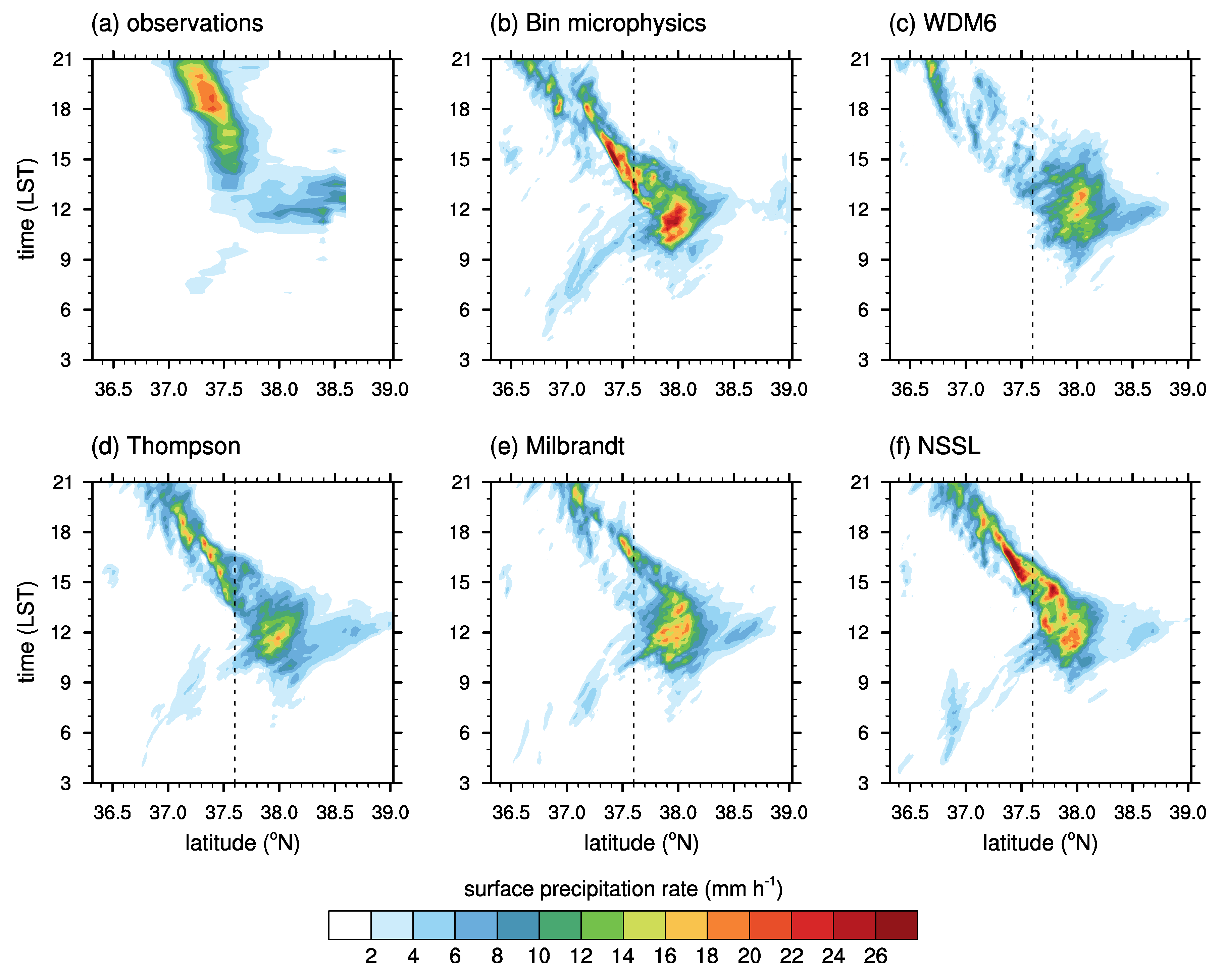
24]. The northern precipitation is not evident in the AWS observations because there are only a small number of AWSs in the region where the actual northern precipitation is concentrated. For the southern precipitation largely concentrated in the region of ~37.0° N—37.5° N and ~127° E—128° E, the bin microphysics scheme simulates strong precipitation that is underestimated and slightly northward biased compared to observations. However, the bin microphysics scheme simulates the location and propagation direction (southeastward) of the strong precipitation similar to observations. On the other hand, all of the bulk microphysics schemes simulate very small amounts of the southern precipitation compared to observations. Among the bulk microphysics schemes, the Thompson–Eidhammer and NSSL schemes simulate the largest amount of the southern precipitation, and the WDM6 scheme simulates the smallest amount of the southern precipitation. The latitude–time diagrams of surface precipitation rate averaged along the longitudinal direction are depicted in
Figure 3. This figure also shows that this precipitation case can be separated into the northern precipitation propagating northward at a relatively fast speed before ~15 LST and the southern precipitation propagating southward at a relatively slow speed after ~15 LST. We note that the observed surface precipitation north of ~38°N seen in
Figure 3a does not well represent real precipitation attributable to the lack of observation stations.
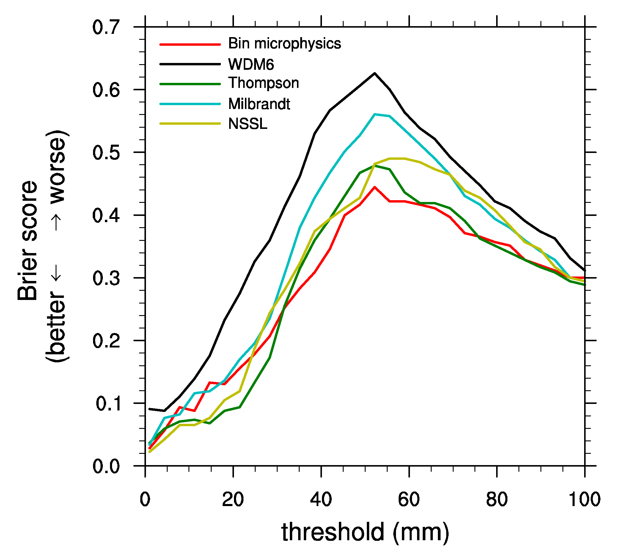
To evaluate the performance of each microphysics scheme in predicting surface precipitation amount more objectively, the Brier score [
45,
46] for the 18-hr accumulated surface precipitation amount is calculated across a range of thresholds (
Figure 4). The Brier score (BS) is defined as:
where
N is the number of comparison points, and
oi and
fi are observation values and forecasting values, respectively. Here, an observation value is defined as unity if the accumulated surface precipitation amount at a given point exceeds the threshold; zero otherwise. There are many methods to define forecasting values, but the same method as that of calculating the observation values is used. Note that different methods to define forecasting values could yield quantitatively different but qualitatively similar results. The Brier scores are low at small thresholds because of the widespread surface precipitation and low at large thresholds because of the limited area of strong surface precipitation.
Figure 4 shows that the Brier score is generally highest (i.e., the model performance is worst) at thresholds of 40–80 mm in this case, and in that range, the bin microphysics scheme shows the best performance among the schemes.
4. Comparison of Bin Microphysics to Bulk Microphysics
In this section, comparisons between the bin microphysics scheme and the four selected bulk microphysics schemes are described.
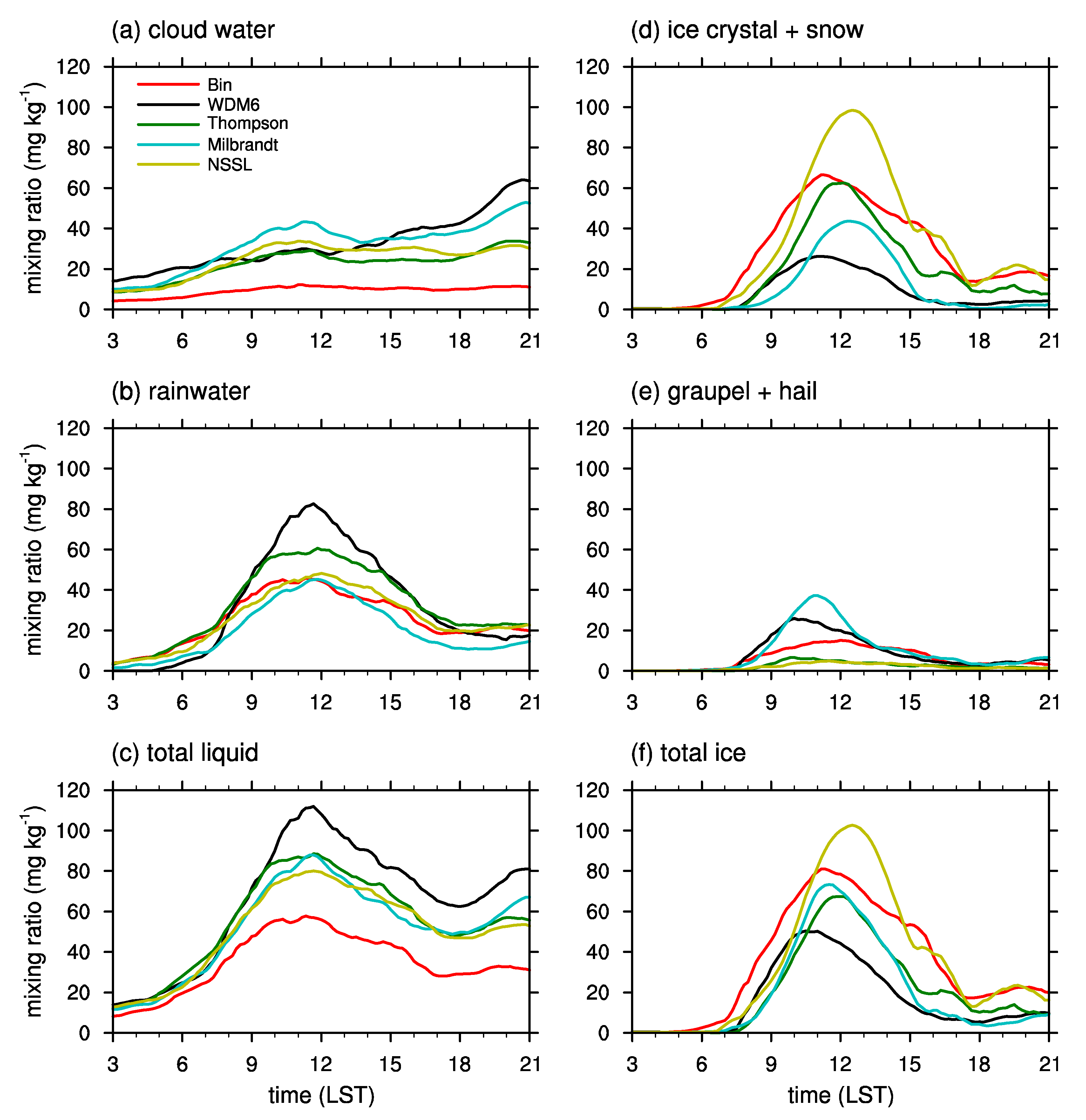
Figure 5 shows the time series of mixing ratios of cloud water, rainwater, pristine and aggregated ice particles (ice crystal and snow), rimed ice particles (graupel and hail), the total liquid water, and the total ice particles. It should be noted that criteria to distinguish hydrometeor types are different depending on the schemes when comparing the mixing ratio of each hydrometeor type from different microphysics schemes.
Among the microphysics schemes, the bin microphysics scheme predicts the smallest cloud water mixing ratio and predicts the largest pristine and aggregated ice particle mixing ratio except the NSSL scheme, and it is one of the schemes that predict the smallest rainwater mixing ratio. In other words, all of the bulk microphysics schemes tend to predict a larger liquid water mixing ratio and a smaller ice particle mixing ratio than the bin microphysics scheme. This suggests that the ice microphysical processes are more active in the bin microphysics scheme than in the bulk microphysics schemes.
While all of the schemes generally predict a relatively smaller rimed ice particle mixing ratio than pristine and aggregated ice particle mixing ratio in this case, the bulk schemes that predict a larger pristine and aggregated ice particle mixing ratio (the NSSL and Thompson–Eidhammer schemes) generally tend to predict a smaller rimed ice particle mixing ratio, and vice versa (the WDM6 and Milbrandt schemes). This implies that the conversion rates from pristine and aggregated ice particles to rimed ice particles might differ greatly depending on the schemes. This so-called type conversion is known to have high uncertainties; even the bin microphysics scheme uses several ad hoc methods to consider the type conversion although it utilizes some additional information (e.g., rimed fractions of snow) to consider the type conversion. A recent alternative approach that predicts ice particle properties [
47] is expected to reduce uncertainties in type conversion.
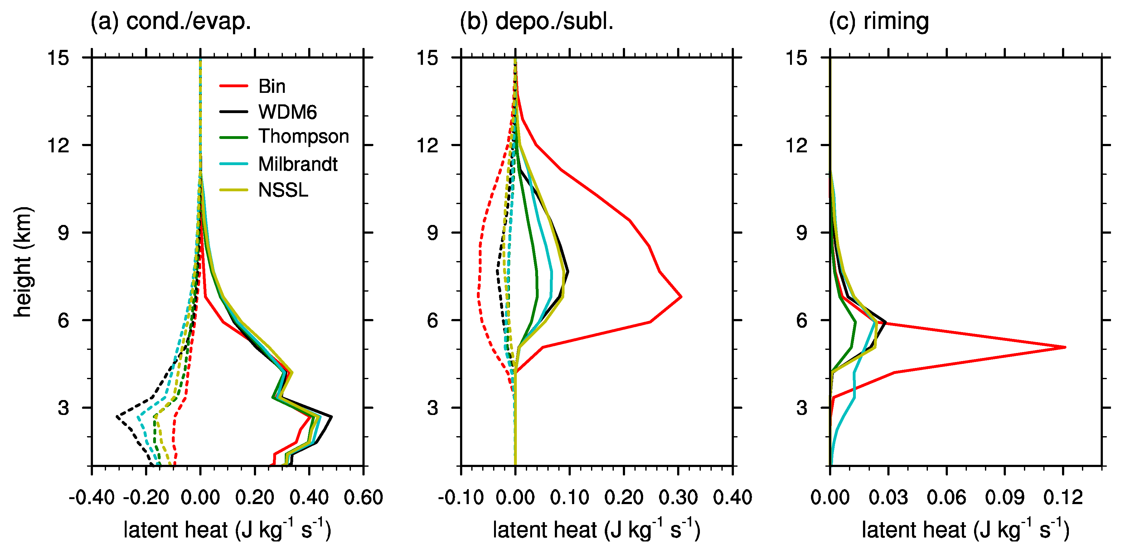
Figure 6 shows the vertical profiles of latent heat release and absorption rates by some selected microphysical processes. All of the examined schemes show similar vertical profiles of condensation and evaporation. The bin microphysics scheme shows the smallest condensation and evaporation below
z ~ 3 km, which is presumably related to the result that the scheme predicts the lowest liquid water mixing ratio among the examined schemes (
Figure 5c). Likewise, the WDM6 scheme, which predicts the largest liquid water mixing ratio, shows the largest condensation and evaporation below
z ~ 3 km.
In contrast to condensation and evaporation, which show similar trends among the schemes, there are distinct differences in deposition, sublimation, and riming between the bin and bulk microphysics schemes. In particular, the bin microphysics scheme shows substantially larger deposition and riming compared to all of the examined bulk microphysics schemes. The latent heat release by deposition and riming in the bin microphysics scheme are more than three times those of the bulk microphysics schemes. The latent heat absorption by sublimation is also largest in the bin microphysics scheme among the examined schemes, but the heating by deposition is much larger than the cooling by sublimation in the bin microphysics scheme as well as in all of the bulk microphysics schemes. Note that the amounts of latent heat release and absorption by other microphysical processes (e.g., freezing and melting) are not large in all the schemes (not shown).
The differences in latent heat release by deposition and riming between the bin and bulk microphysics schemes are likely to alter the development of clouds and precipitation.
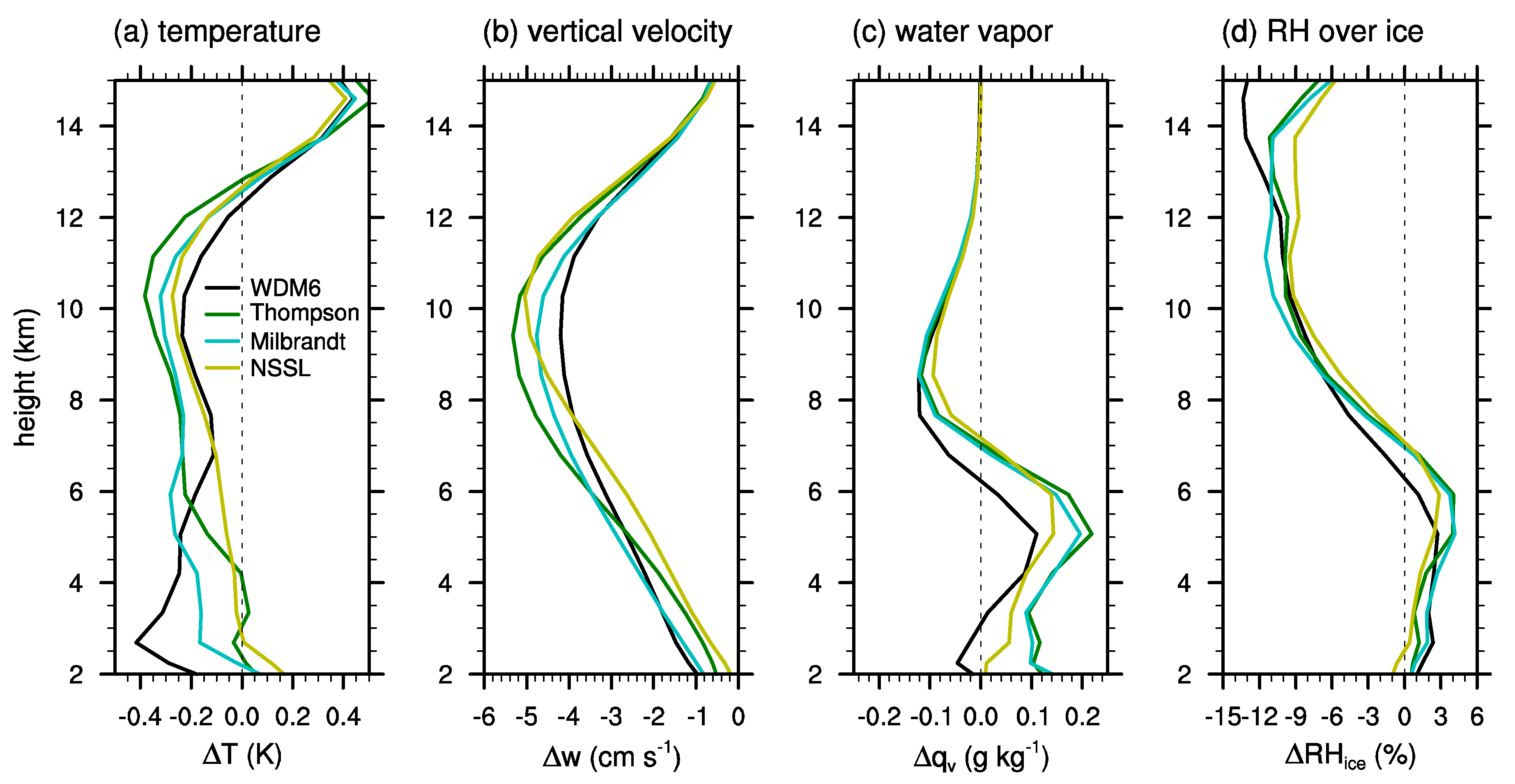
Figure 7 shows the deviations of some selected atmospheric variables, which are temperature, vertical velocity, water vapor mixing ratio, and relative humidity with respect to ice, obtained using the bulk microphysics schemes from those obtained using the bin microphysics scheme. It is clearly seen that all of the bulk microphysics schemes show a lower temperature in the layer between ~4–12 km and weaker vertical velocity in all layers compared to the bin microphysics scheme. In addition, all of the bulk microphysics schemes generally show more water vapor in the lower layer (below ~6 or 7 km) but less water vapor in the upper layer than the bin microphysics scheme. Although the decrease in water vapor in the upper layer is similar in magnitude to the increase in the lower layer (
Figure 7c), the decrease in relative humidity in the upper layer is more pronounced than the increase in the lower layer (
Figure 7d). This is simply because the water vapor mixing ratio in the upper layer is much smaller than that in the lower layer.
The latent heat release, upward motion, and vapor diffusional growth are closely related to each other in cloud development. Once the temperature rises due to the latent heat release, the upward motion becomes stronger, and the stronger upward motions transport more water vapor from the lower layer to the upper layer. The transported water vapor prompts an increase in vapor diffusional growth of ice particles, which causes more latent heat release and a further rise in temperature. In this case, the bin microphysics scheme predicts a distinctly larger amount of latent heat release by deposition and riming compared to the bulk microphysics schemes (
Figure 6). This larger latent heat release in the bin microphysics scheme causes the increases in temperature, vertical velocity, and upper-layer water vapor mixing ratio (
Figure 7). The latent heat release is again amplified by the increased vapor diffusional growth in the upper layer. Note that the increased vertical velocity in the bin microphysics scheme might also affect the relatively small cloud water mixing ratio and relatively large pristine and aggregated ice particle mixing ratio (
Figure 5a,d). The increased vertical velocity can transport more amount of cloud water from the lower layer, which can form more ice crystals in the upper layer.
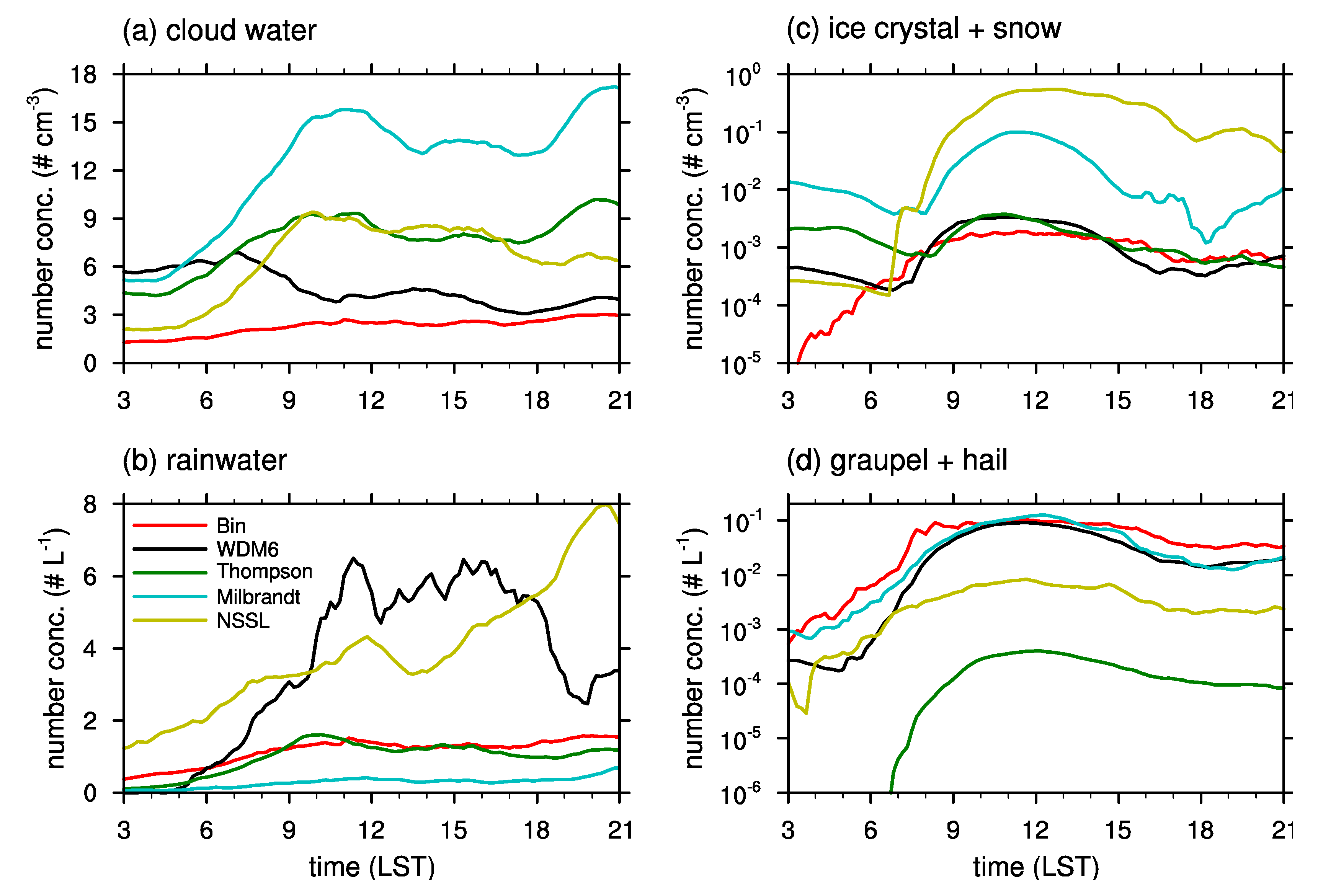
Figure 8 shows the time series of number concentrations of cloud water, rainwater, pristine and aggregated ice particles, and rimed ice particles. It is easily seen that the differences among the schemes are larger in terms of hydrometeor number concentration than in terms of hydrometeor mixing ratio (
Figure 5). Moreover, the relative differences in ice particle number concentrations among the schemes are much larger than those of liquid particles. The NSSL and Milbrandt schemes yield the number concentrations of pristine and aggregated ice particles that are larger by several orders compared to those of the bin microphysics scheme, which would result in smaller ice particles. The Thompson–Eidhammer and NSSL schemes, which predict the smallest rimed ice particle mixing ratio among the schemes (
Figure 5e), predict the significantly small number concentrations of rimed ice particles. These large differences in the hydrometeor number concentrations among the schemes simply show that uncertainties in predicting the number concentrations of hydrometeors, particularly of ice particles, are larger than those of the mixing ratios. There are relatively less studies that report reliable observational statistics on the hydrometeor number concentration. Because the hydrometeor number concentration is used to estimate a representative size of particles that is essential for calculating microphysical processes, these large uncertainties in predicting hydrometeor number concentration should be improved in future studies (e.g., [
48]).
It was discussed in
Figure 6 and
Figure 7 that the bin microphysics scheme exhibits a larger latent heat release by deposition and riming compared to the examined bulk microphysics schemes and that this increased latent heat release enhances vertical motion. To investigate whether this enhanced convection is associated with the better performance in predicting the surface precipitation in the case considered in this study than that of the bulk microphysics schemes (
Figure 2,
Figure 3 and
Figure 4), an additional simulation with a small modification of the bin microphysics scheme, which excludes the riming of cloud droplets onto ice crystals, is conducted. It is noted that the collision between ice crystals and cloud droplets is not considered in all the bulk microphysics schemes chosen in this study except the NSSL scheme, presumably because ice crystals and cloud droplets are generally regarded as non-sedimenting particles in bulk microphysics schemes. By excluding the riming of cloud droplets onto ice crystals, it is expected that the latent heat release attributable to riming would be decreased.
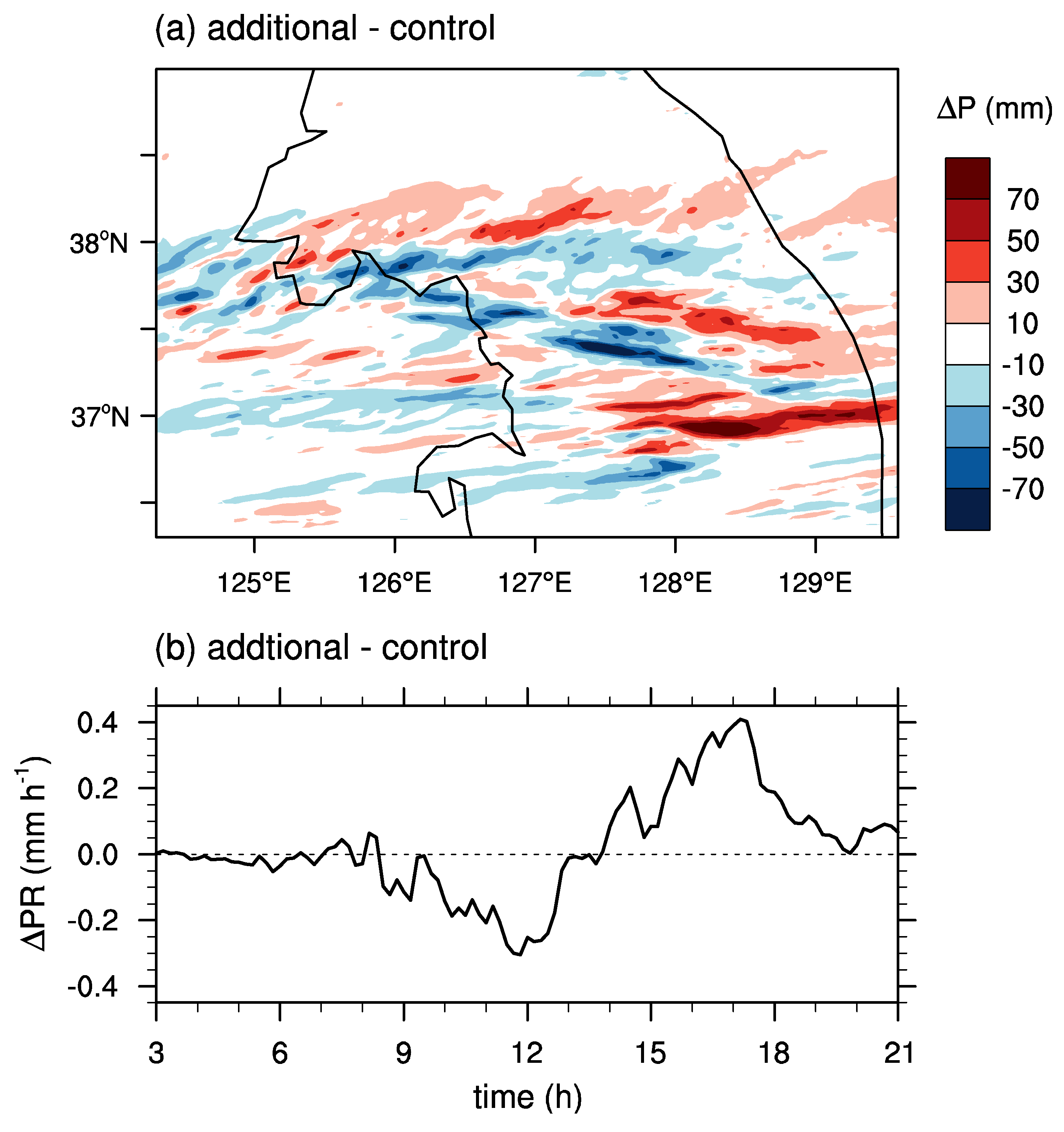
Figure 9 shows the differences in surface precipitation between the additional simulation and the control simulation (conducted using the original bin microphysics scheme). The southern precipitation in the region of ~37.0° N—37.6° N and ~126.5° E—129° E (see
Figure 2b) is slightly weakened and shifted eastward. The time series of the difference in surface precipitation rate (
Figure 9b) shows that the surface precipitation rate in the additional simulation is lower than that of the control simulation before ~13 LST.
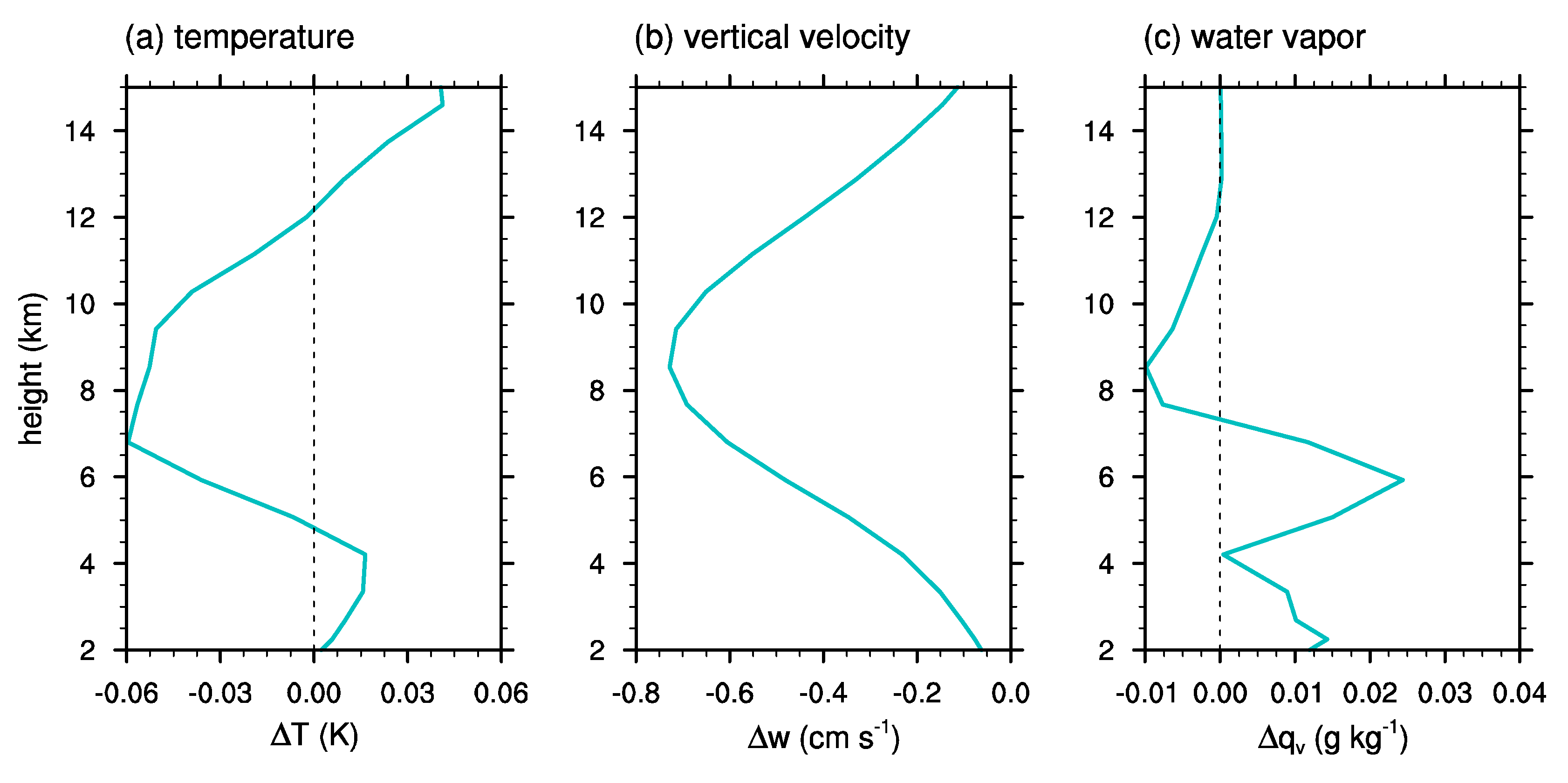
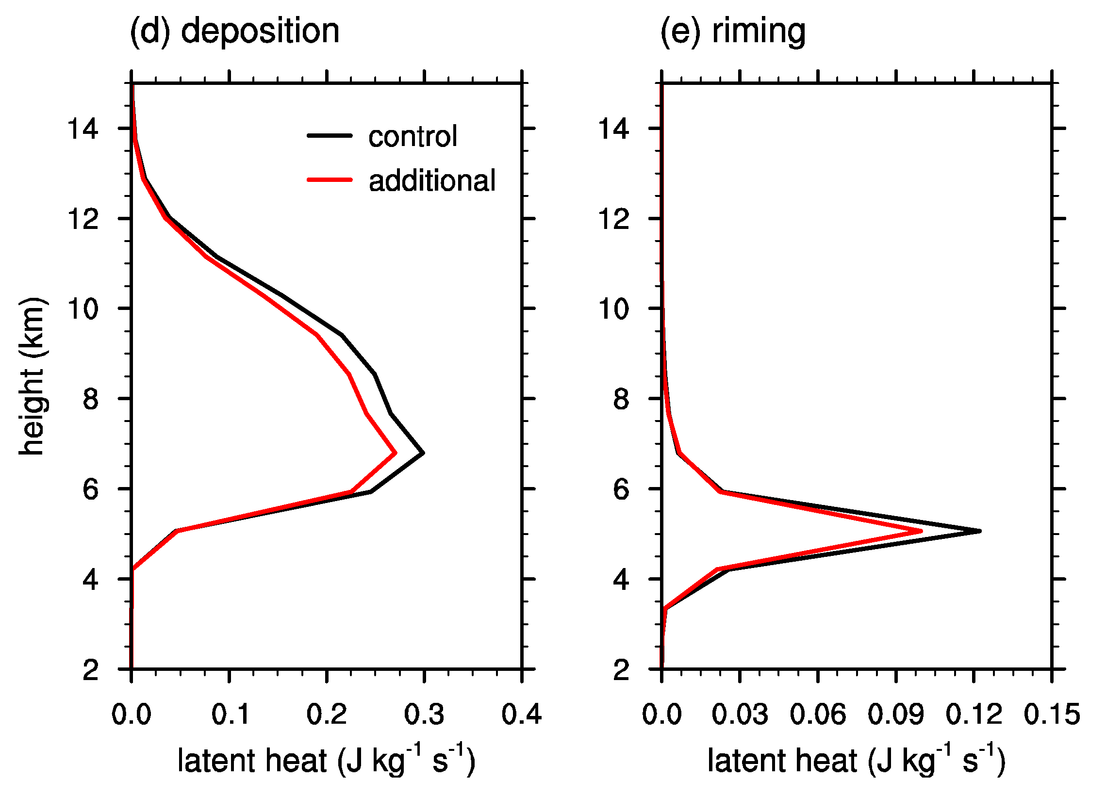
Figure 10 shows the vertical profiles of deviations in temperature, vertical velocity, and water vapor mixing ratio obtained in the additional simulation from those that are obtained in the control simulation, and the vertical profiles of latent heat release by deposition and riming. The profiles are obtained by averaging from 03 LST to 13 LST. It is clearly seen that the overall trends shown in
Figure 10a–c are almost the same as shown in
Figure 7a–c. In the additional simulation, the temperature in the upper level (~5–12 km) is decreased, the vertical velocity is decreased in the entire layer, and the upper-level (~7–12 km) water vapor mixing ratio is decreased. In addition,
Figure 10d,e shows that deposition as well as riming is decreased in the additional simulation. Therefore, it can be concluded that by excluding the riming of cloud droplets onto ice crystals, latent heat release by riming and deposition is decreased, which causes the decreases in upper-level temperature, vertical velocity, and upper-level water vapor. These decreases seem to be associated with the slight decrease in surface precipitation amount and the shift of precipitation toward the downwind side (
Figure 9), presumably attributable to the decrease in the convective activity and the growth of ice particles.
On the other hand, after ~14 LST, the surface precipitation rate increases in the additional simulation although the riming of cloud droplets on ice crystals is excluded. The accumulated surface precipitation amount is clearly increased in the region of ~37° N and ~128° E–129.5° E (
Figure 9a). This can be explained by considering that the remaining small ice crystals and cloud droplets in clouds grow further by vapor diffusion, hence inducing an increase in vertical velocity and surface precipitation at the later stage. Our further analysis shows that latent heat releases by deposition and riming increase and upper-level temperature, vertical velocity, and upper-level water vapor mixing ratio are also enhanced in the additional simulation (not shown), contrary to the results before 13 LST. Therefore, the relationship between the surface precipitation and convective activity represented as latent heat release and vertical velocity remains similar even after ~14 LST.
5. Summary and Conclusions
This study compared the bin and bulk microphysics schemes by conducting numerical simulations for a real precipitation case using the WRF model. We implemented the bin microphysics scheme of the Hebrew University Cloud Model (somewhat different from the publicly available version) in the WRF model. Four bulk microphysics schemes in the WRF model (the WDM6 scheme, Thompson–Eidhammer scheme, Milbrandt scheme, and NSSL scheme), which are double-moment for liquid drops, were selected. Using the WRF model, the precipitation event that occurred on 21 September 2010 in the central Korean Peninsula was numerically simulated.
While all of the microphysics schemes underestimate the strong precipitation shown in the AWS observations, the bin microphysics scheme simulates the largest amount of the accumulated surface precipitation, which is the closest to observations. All of the bulk microphysics schemes tend to predict a larger liquid water mixing ratio and a smaller ice particle mixing ratio compared to the bin microphysics scheme, which might be partially contributed to by weaker vertical velocity in the bulk microphysics schemes. The bulk microphysics schemes that exhibit a larger rimed ice particle mixing ratio tend to exhibit a smaller pristine and aggregated ice particle mixing ratio, which implies that the conversion rates in the bulk microphysics schemes are substantially different depending on the schemes. In addition, the differences in hydrometeor number concentration among the schemes are larger than those of mixing ratio, which needs to be improved in future studies (e.g., [
49]).
It was shown that all of the bulk microphysics schemes predict much smaller latent heat release by deposition and riming compared to the bin microphysics scheme. Also, they predict lower temperature, weaker vertical velocity, and smaller upper-level water vapor mixing ratio than the bin microphysics scheme in this case. The increased latent heat release can enhance itself again through the enhanced upward transport of moisture. It is found that no bulk microphysics schemes examined in this study, except the NSSL scheme, consider the growth of ice crystals by colliding with cloud droplets, presumably owing to their negligible fall velocities. The exclusion of this riming process in the bulk microphysics schemes might contribute to the underestimation of air temperature, vertical velocity, and upper-level water vapor mixing ratio compared to those of the bin microphysics scheme. An additional simulation with the bin microphysics scheme, in which the riming of cloud droplets onto ice crystals is excluded, revealed that the simulated surface precipitation is slightly decreased and moved to the downwind side compared to the control simulation conducted using the original bin microphysics scheme before a certain time instance. Before the time instance, the additional simulation exhibits the decreased deposition, riming, upper-level temperature, vertical velocity, and upper-level water vapor mixing ratio, which are very similar to those shown in the comparisons of the bulk and bin microphysics schemes. After the time instance, the results are reversed; deposition, riming, upper-level temperature, vertical velocity, and upper-level water vapor mixing ratio increase in the additional simulation compared to those of the control simulation, which is presumably attributable to the further vapor diffusional growth of small ice crystals aloft. The surface precipitation amount after the time instance is larger in the additional simulation, so the relationship between convective activity, which is represented as vertical velocity and vapor diffusion, and surface precipitation is still valid.
Previous studies have mainly focused on the fundamental differences between bin and bulk microphysics schemes in expressing the size distributions of cloud particles, and they have attempted to improve bulk microphysics schemes through a better representation of particle size distributions [
30,
50]. This study shows that a more appropriate representation of microphysical processes in bin microphysics scheme than in bulk microphysics schemes can contribute to more accurate prediction in this real precipitation case. Therefore, certain oversimplified assumptions in treating microphysical processes of traditional bulk microphysics schemes (e.g., ignoring the terminal velocities of cloud droplets and ice crystals and the collision between cloud droplets and ice crystals) need to be revised and constrained by detailed observations [
48] to improve the performance of bulk microphysics schemes. This can help better understanding and prediction of precipitation.


