Observed Key Surface Parameters for Characterizing Land–Atmospheric Interactions in the Northern Marginal Zone of the Taklimakan Desert, China

 , ,
, ,
Abstract
1. Introduction
2. Observational Site and Analytical Methods
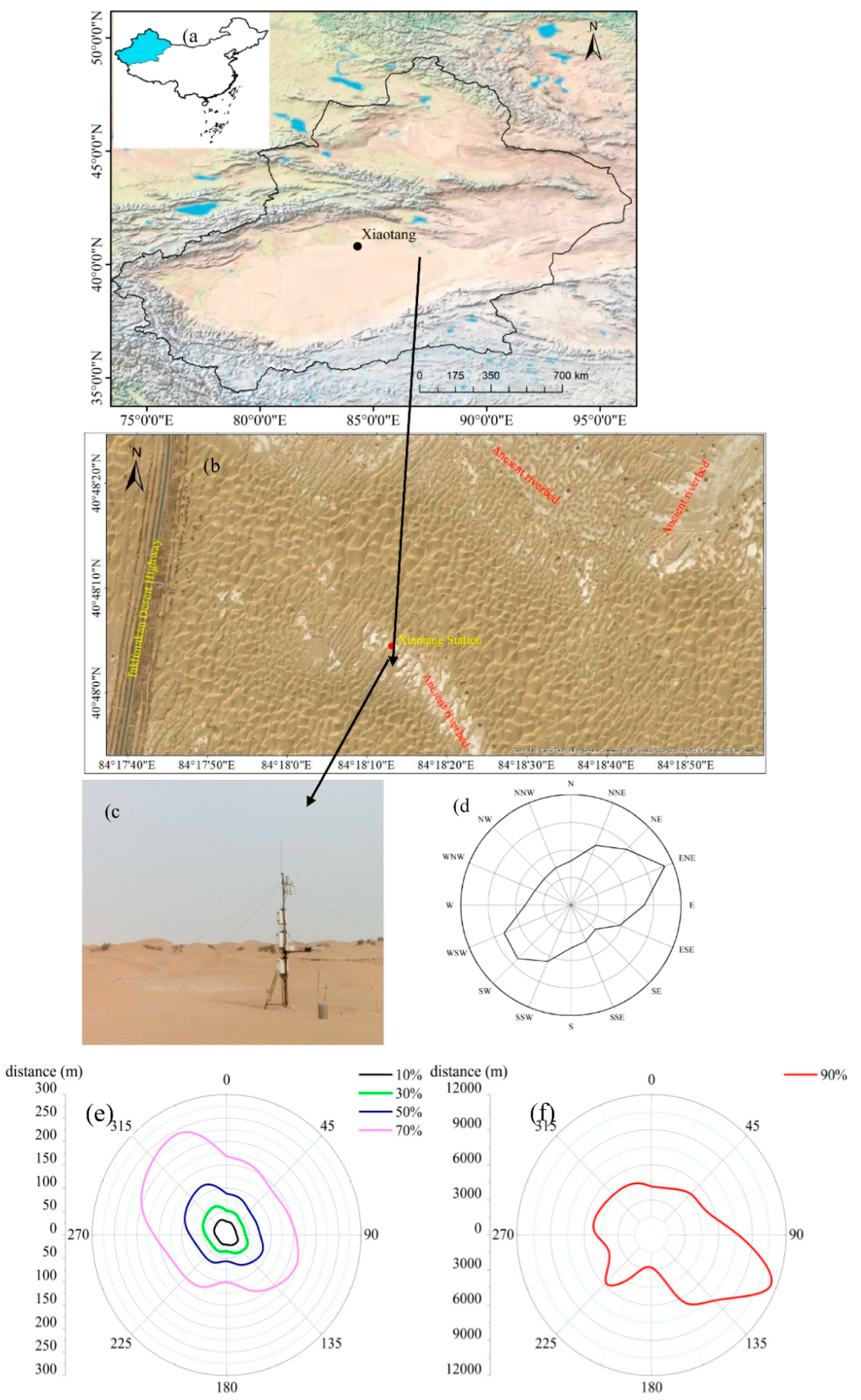
2.1. Site Description
2.2. Data
2.3. Theory and Methodology
3. Results and Discussion
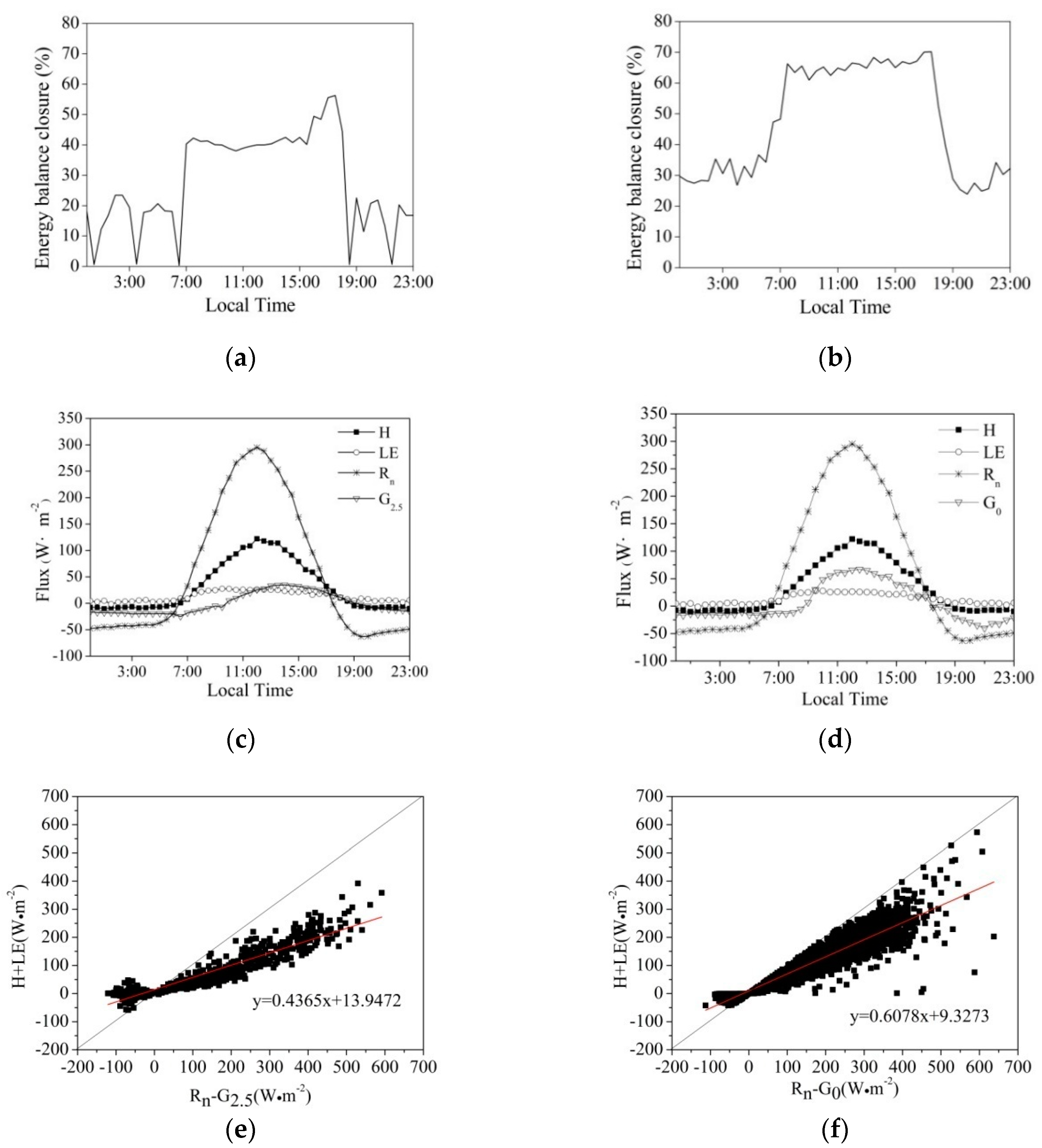
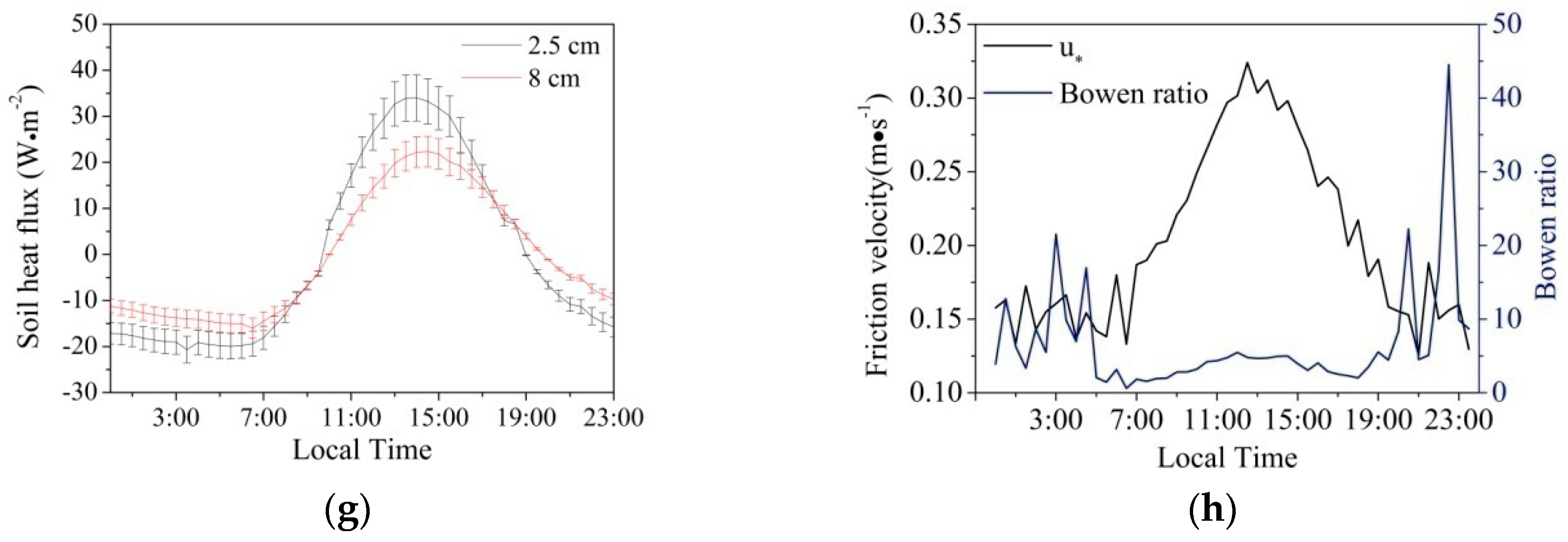
3.1. Surface Energy Balance Closure
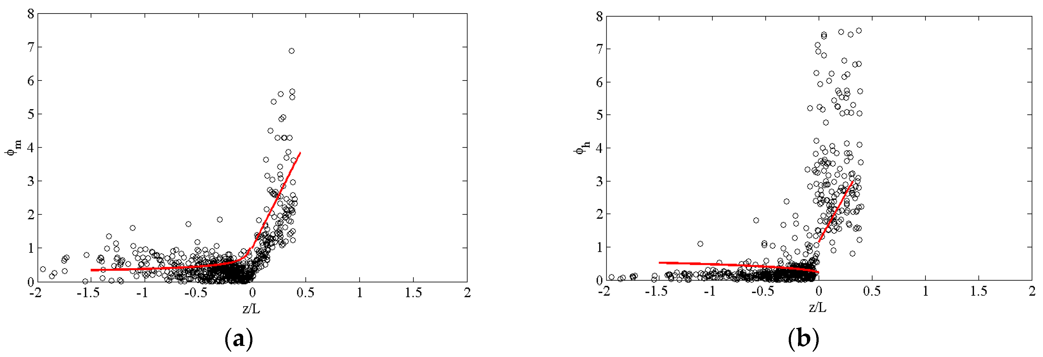
3.2. Relationships between φm, φh, and z/L
3.3. Surface Albedo
3.4. Surface Emissivity
3.5. Aerodynamic Roughness Length (z0m), Thermal Roughness Length (z0h), and kB−1
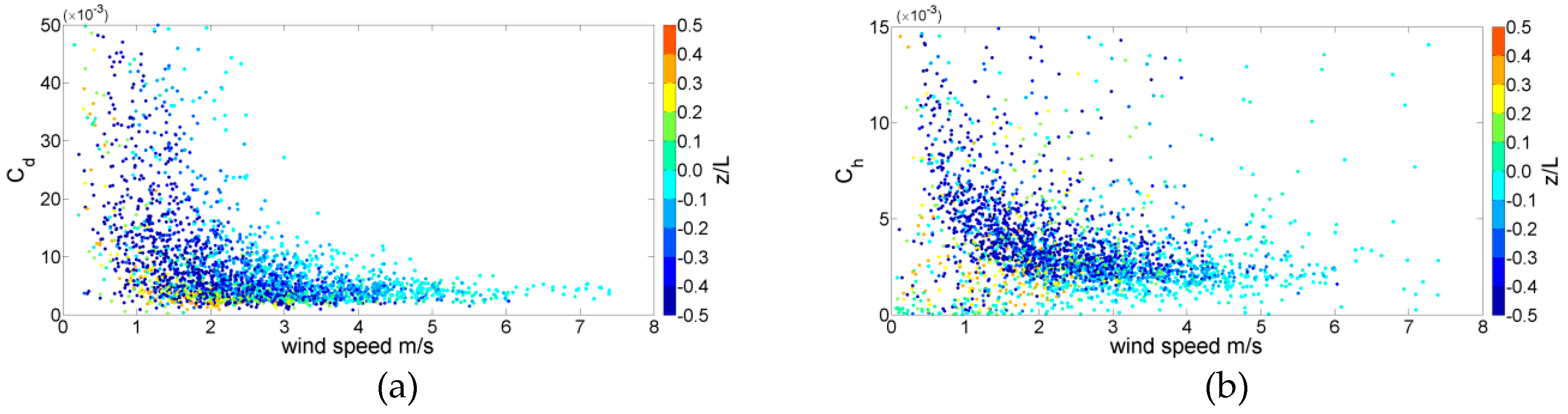
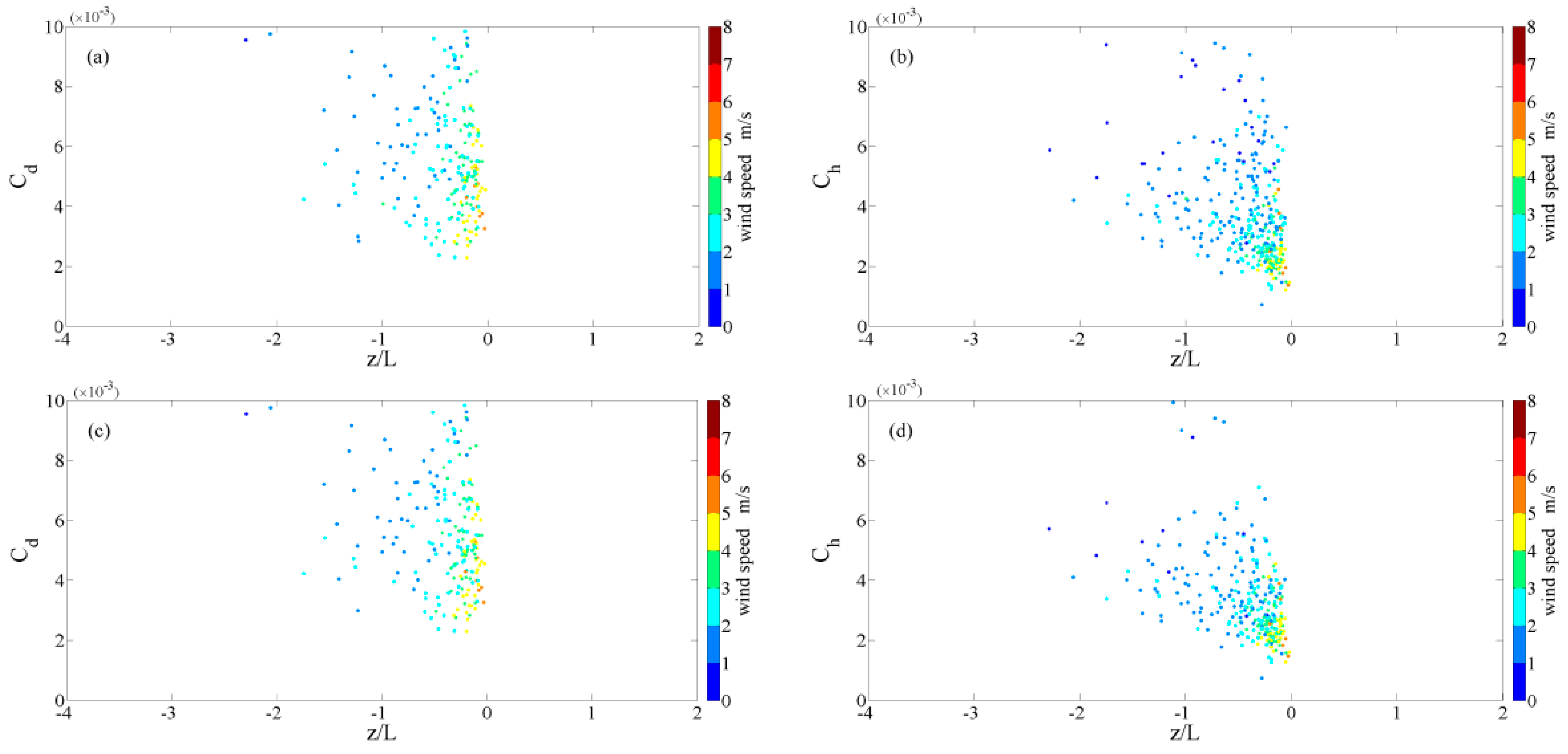
3.6. Bulk Transfer Coefficients Cd and Ch
4. Discussion
5. Conclusions and Further Work
Author Contributions
Funding
Conflicts of Interest
References
- Zeng, X.B.; Shaikh, M.; Dai, Y.J.; Dickinson, R.E.; Myneni, R. Coupling of the common land model to the NCAR community climate model. J. Clim. 2002, 15, 1832–1854. [Google Scholar] [CrossRef]
- Li, J.Y.; Ye, C.Z.; Zhong, Z. Impacts of land-surface process parameterization on model predictability of two kinds of heavy rainfall events. Chin. J. Atmos. Sci. 2010, 34, 407–417. (In Chinese) [Google Scholar]
- Stull, R.B. An Introduction to Boundary Layer Meteorology; Kluwer Academic Publishers: Dordrecht, The Netherlands, 1988; pp. 383–385. [Google Scholar]
- Garratt, J.R. Review of drag coefficients over oceans and continents. Mon. Weather Rev. 1977, 105, 915–929. [Google Scholar] [CrossRef]
- Tomoaki, O. Seasonal change of Asian summer monsoon circulation and its heat source. J. Meteorol. Soc. Jpn. 1998, 76, 1045–1063. [Google Scholar]
- Tzeng, R.Y.; Lee, Y.H. The effects of land-surface characteristics on the East Asian summer monsoon. Clim. Dynam. 2001, 17, 317–326. [Google Scholar] [CrossRef]
- Boussetta, S.; Balsamo, G.; Dutra, E.; Beljaars, A.; Albergel, C. Assimilation of surface albedo and vegetation states from satellite observations and their impact on numerical weather prediction. Remote Sens. Environ. 2015, 163, 111–126. [Google Scholar] [CrossRef]
- Liu, Y.Q.; He, Q.; Zhang, H.S.; Mamtimin, A. Improving the CoLM in Taklimakan Desert hinterland with accurate key parameters and an appropriate parameterization scheme. Adv. Atmos. Sci. 2012, 29, 381–390. [Google Scholar] [CrossRef]
- Feldman, D.R.; Collins, W.D.; Pincus, R.; Huang, X.L.; Chen, X.H. Far-infrared surface emissivity and climate. Proc. Natl. Acad. Sci. USA 2014, 111, 16297–16302. [Google Scholar] [CrossRef] [PubMed]
- Garratt, J.R. Flux profile relations above tall vegetation. Q. J. R. Meteorol. Soc. 1978, 104, 199–211. [Google Scholar] [CrossRef]
- Yang, K.; Koike, T.; Ishikawa, H.; Kim, J.; Li, X.; Liu, H.Z.; Liu, S.M.; Ma, Y.M.; Wang, J.M. Turbulent flux transfer over bare-soil surfaces: Characteristics and parameterization. J. Appl. Meteorol. Clim. 2008, 47, 276–290. [Google Scholar] [CrossRef]
- Lu, L.; Liu, S.M.; Xu, Z.W.; Yang, K.; Cai, X.H.; Jia, L.; Wang, J.M. The characteristics and parameterization of aerodynamic roughness length over heterogeneous surfaces. Adv. Atmos. Sci. 2009, 26, 180–190. [Google Scholar] [CrossRef]
- Toda, M.; Sugita, M. Single level turbulence measurements to determine roughness parameters of complex terrain. J. Geophys. Res. Atmos. 2003, 108. [Google Scholar] [CrossRef]
- Brock, B.W.; Willis, I.C.; Sharp, M.J. Measurement and parameterization of aerodynamic roughness length variations at Haut Glacier d’Arolla, Switzerland. J. Glaciol. 2006, 52, 281–297. [Google Scholar] [CrossRef]
- Paul, G.; Gowda, P.H.; Prasad, P.V.V.; Howell, T.A.; Aiken, R.M.; Neale, C.M.U. Investigating the influence of roughness length for heat transport (zoh) on theperformance of SEBAL in semi-arid irrigated and dryland agricultural systems. J. Hydrol. 2014, 509, 231–244. [Google Scholar] [CrossRef]
- Zheng, D.H.; Velde, R.V.D.; Su, Z.B.; Booij, M.J.; Hoekstra, A.Y.; Wen, J. Assessment of roughness length schemes implemented within the Noah land surface model for high-altitude regions. J. Hydrometeorol. 2014, 15, 921–937. [Google Scholar] [CrossRef]
- Zhang, Q.; Yao, T.; Yue, P. Development and test of a multifactorial parameterization scheme of land surface aerodynamic roughness length for flat land surfaces with short vegetation. Sci. China Earth Sci. 2016, 59, 281–295. [Google Scholar] [CrossRef]
- Banerjee, T.; De Roo, F.; Mauder, M. Explaining the convector effect in canopy turbulence by means of large-eddy simulation. Hydrol. Earth Syst. Sci. 2017, 21, 2987–3000. [Google Scholar] [CrossRef]
- Mauder, M.; Genzel, S.; Fu, J.; Kiese, R.; Soltani, M.; Steinbrecher, R.; Zeeman, M.; Banerjee, T.; de Roo, F.; Kunstmann, H. Evaluation of energy balance closure adjustment methods by independent evapotranspiration estimates from lysimeters and hydrological simulations. Hydrol. Process. 2018, 32, 39–50. [Google Scholar] [CrossRef]
- Graf, A.; van de Boer, A.; Moene, A.; Vereecken, H. Intercomparison of methods for the simultaneous estimation of zero-plane displacement and aerodynamic roughness length from single-level eddy-covariance data. Bound.-Layer Meteorol. 2014, 151, 373–387. [Google Scholar] [CrossRef]
- Chen, Q.T.; Jia, L.; Hutjes, R.; Menenti, M. Estimation of aerodynamic roughness length over oasis in the Heihe River Basin by utilizing remote sensing and ground data. Remote Sens. 2015, 7, 3690–3709. [Google Scholar] [CrossRef]
- Miao, M.Q.; Qian, J.P. Characteristics of bulk transfer coefficient and transport coefficient over the land. Acta Meteorol. Sin. 1996, 54, 95–101. [Google Scholar]
- Verhoef, A.; de Bruin, H.A.R.; van den Hurk, B. Some practical notes on the parameter kB–1 for sparse vegetation. J. Appl. Meteorol. 1997, 36, 560–572. [Google Scholar] [CrossRef]
- Sun, J. Diurnal variations of thermal roughness height over a grassland. Bound.-Layer Meteorol. 1999, 92, 407–427. [Google Scholar] [CrossRef]
- Ma, Y.; Tsukamoto, O.; Wang, J.M.; Hirohiko, I.; Ichiro, T. Analysis of aerodynamic and thermodynamic parameters on the grassy marshland surface of Tibetan Plateau. Prog. Nat. Sci. 2002, 12, 36–40. [Google Scholar]
- Chen, Y.Y.; Yang, K.; Zhou, D.G.; Qin, J.; Guo, X.F. Improving the Noah land surface model in arid regions with an appropriate parameterization of the thermal roughness length. J. Hydrometeorol. 2010, 11, 995–1006. [Google Scholar] [CrossRef]
- Charney, J.G. Dynamics of deserts and drought in the Sahel. Q. J. R. Meteorol. Soc. 1975, 101, 193–202. [Google Scholar] [CrossRef]
- Ta, Y.E.; Lü, X.; Ma, L.H.; Ding, L.J. Study on change of net radiation radiation and heat flux in south oasis of Gurbantunggut Desert. J. Shihezi Univ. (Nat. Sci.) 2005, 23, 587–590. (In Chinese) [Google Scholar]
- Cunnington, W.M.; Rowntree, P.R. Simulations of the Saharan atmosphere-dependence on moisture and albedo. Q. J. R. Meteorol. Soc. 1986, 112, 971–999. [Google Scholar]
- Kimura, F.; Shimizu, Y. Estimation of sensible and latent heat fluxes from soil surface temperature using a linear air-land heat transfer model. J. Appl. Meteorol. 1994, 33, 477–489. [Google Scholar] [CrossRef]
- Wei, W.S.; Dong, G.R. Radiant heat transportation at the interface of desert-taking Gurbantunggut desert for example. Acta Sedimentol. Sin. 1999, 17, 840–845. (In Chinese) [Google Scholar]
- Li, G.P.; Duan, T.Y.; Haginoya, S.; Chen, L.X. Estimates of the bulk transfer coefficients and surface fluxes over the Tibetan Plateau using AWS data. J. Meteorol. Soc. Jpn. 2001, 79, 625–635. [Google Scholar] [CrossRef]
- Wang, M.Z.; Wei, W.S.; Yang, L.M.; He, Q.; Geng, Y. Analysis on space-time characteristics of surface latent heat flux in Taklimakan Desert. J. Desert Res. 2008, 28, 940–947. (In Chinese) [Google Scholar]
- Wang, M.Z.; Yang, L.M.; Wei, W.S.; He, Q.; Geng, Y.; Li, H.J. Analysis on characteristics of surface sensible heat flux in Taklimakan Desert. J. Arid Land Resour. Environ. 2009, 23, 172–178. (In Chinese) [Google Scholar]
- He, Q.; Zhao, J.F. Studies on the distribution of floating dusts in Tarim Basin. Chin. J. Arid Land Res. 1999, 12, 35–42. [Google Scholar]
- Liu, Y.Q.; He, Q.; Zhang, H.S.; Mamtimin, A. Studies of land-atmosphere interaction parameters in Taklimakan Desert hinterland. Plateau Meteorol. 2011, 30, 1294–1299. (In Chinese) [Google Scholar]
- Liu, Y.Q.; Mamtimin, A.; He, Q. Estimation of the surface roughness length and bulk transfer coefficients over the hinterland of Taklimakan Desert. IJAES 2013, 8, 1401–1411. [Google Scholar]
- Jin, L.L.; Li, Z.J.; Mamtimin, A.; He, Q.; Liu, Y.Q. Characteristics and Parameterization Scheme of Surface Albedo Over the Northern Margin of the Taklimakan Desert. Resour. Sci. 2014, 36, 1051–1061. (In Chinese) [Google Scholar]
- Qian, Z.A.; Song, M.H.; Li, W.Y. Analyses on distributive variation and forecast of sand-dust storms in recent 50 years in North China. J. Desert Res. 2002, 2, 106–111. [Google Scholar]
- Warner, T.T. Desert Meteorology; Wei, W.S.; Cui, C.X.; Shang, H.M.; He, Q.; Liu, Y.; Yang, L.M.; Liu, X.C.; Zhang, G.X.; Wang, J.; Nan, Q.H.; et al., Translators; Cambridge University Press: Cambridge, UK, 2004; Volume 197, 595p. (In Chinese) [Google Scholar]
- Sun, J.M.; Liu, T.S. The age of the Taklimakan Desert. Science 2006, 312, 1621. [Google Scholar] [CrossRef] [PubMed]
- Miller, R.L.; Tegen, I. Climate response to soil dust aerosols. J. Clim. 1998, 11, 3247–3267. [Google Scholar] [CrossRef]
- Washington, R.; Todd, M.; Middleton, N.J.; Goudie, A.S. Dust-storm source determined by the total ozone monitoring spectrometer and surface observations. Ann. Assoc. Am. Geogr. 2003, 93, 297–313. [Google Scholar] [CrossRef]
- Liu, Y.Q.; Mamtimin, A.; Huo, W.; Yang, X.H.; Liu, X.C.; Meng, X.Y.; He, Q. Estimation of the land surface emissivity in the hinterland of Taklimakan Desert. J. Mt. Sci. 2014, 11, 1543–1551. [Google Scholar] [CrossRef]
- Korb, A.R.; Salisbury, J.W.; D’Aria, D.M. Thermal-infrared remote sensing and Kirchhoff’s law: 2. Field measurements. J. Geophys. Res. 1999, 104, 15339–15350. [Google Scholar] [CrossRef]
- Korb, A.R.; Dybwad, P.; Wadsworth, W.; Salisbury, J.W. Portable Fourier transform infrared spectrometer for field measurements of radiance and emissivity. Appl. Opt. 1996, 35, 1679–1692. [Google Scholar] [CrossRef] [PubMed]
- Ma, D.; Lü, S.H.; Chen, S.Q.; Luo, S.Q.; Quan, X.J. Distribution of source area and footprint of Jinta Oasis in summer. Plateau Meteorol. 2009, 28, 28–35. (In Chinese) [Google Scholar]
- Yang, K.; Wang, J.M. A Correction method for temperature prediction that calculate surface soil heat flux based on soil temperature and humidity data. Sci. China Press 2008, 38, 243–250. (in Chinese). [Google Scholar]
- Wilson, K.; Goldstein, A.; Falge, E.; Aubinet, M.; Baldocchi, D. Energy Balance Closure at FLUXNET Sites. Agric. For. Meteorol. 2002, 113, 223–243. [Google Scholar] [CrossRef]
- Stoy, P.C.; Mauder, M.; Foken, T.; Barbara, M.; Eva, B.; Andreas, I.; Altaf, A.M.; Lu, A.A.; Mika, A.; Christian, B. A data-driven analysis of energy closure across FLUXNET research sites: The role of landscape scale heterogeneity. Agric. For. Meteorol. 2013, 171–172, 137–152. [Google Scholar] [CrossRef]
- Huang, R.H.; Chen, W.; Ma, Y.M.; Gao, X.Q.; Lü, S.H.; Wei, Z.G.; Zhang, Q.; Wei, G.A.; Hu, Z.Y.; Zhou, L.T.; et al. Land Atmosphere Interaction and Its Effect on East Asian Climate Change in Arid Region in the Northwest of China; Meteorol Press: Beijing, China, 2011; 100p. (In Chinese) [Google Scholar]
- Dyer, A.J. A review of flux-profile relationships. Bound.-Layer Meteorol. 1974, 7, 363–372. [Google Scholar] [CrossRef]
- Paulson, C.A. The mathematical representation of wind speed and temperature profiles in the unstable atmospheric surface layer. J. Appl. Meteorol. 1970, 9, 857–861. [Google Scholar] [CrossRef]
- Webb, E.K. Profile relationships: The log-linear range, and extension to strong stability. Q. J. R. Meteorol. Soc. 1970, 96, 67–90. [Google Scholar] [CrossRef]
- Businger, J.A.; Wyngaard, J.C.; Izumi, Y.; Bradley, E.F. Flux-profile relationships in the atmospheric surface layer. J. Atmos. Sci. 1971, 28, 181–189. [Google Scholar] [CrossRef]
- Kanda, M.; Kanega, M.; Kawai, T.; Moriwaki, R. Roughness lengths for momentum and heat derived from outdoor urban scale models. J. Appl. Meteorol. Clim. 2007, 46, 1067–1079. [Google Scholar] [CrossRef]
- Heikinheimo, M.; Kangas, M.; Tourule, T.; Venäläinena, A.; Tattari, S. Momentum and heat fluxes over lakes Tämnaren and Råksjö determined by the bulk-aerodynamic and eddy-correlation methods. Agric. For. Meteorol. 1999, 98–99, 521–534. [Google Scholar] [CrossRef]
- Mahrt, L.; Vickers, D. Bulk formulation of the surface heat flux. Bound.-Layer Meteorol. 2003, 110, 357–379. [Google Scholar] [CrossRef]
- Qin, Z.H.; Li, W.J.; Xu, B.; Chen, Z.X.; Liu, J. The estimation of land surface emissivity for Landsat TM6. Remote Sens. Land Resour. 2004, 61, 28–32, 36, 41. (In Chinese) [Google Scholar]
- Zuo, H.C.; Hu, Y.Q. The bulk transfer coefficient over desert and gobi in HEIFE region. Plateau Meteorol. 1992, 11, 371–380. (In Chinese) [Google Scholar]
- Zhang, Q.; Huang, R.H.; Wang, S.; Wei, G.A.; Cao, X.Y.; Hou, X.H.; Lü, S.H.; Hu, Z.Y.; Ma, Y.M.; Wei, Z.G.; et al. NWC-ALIEX and IEX research advances. Adv. Earth Sci. 2005, 20, 427–441. (In Chinese) [Google Scholar]
- Zheng, H.; Liu, S.H. Land surface parameterization and modeling over desert. Chin. J. Geophys. 2013, 56, 2207–2217. (In Chinese) [Google Scholar]
- Stull, R.B. Introduction to Boundry Layer Meteorology; Yang, C., Translator; Meteorological Press: Beijing, China, 1991; pp. 719–720. (In Chinese) [Google Scholar]
- Zou, J.L.; Hou, X.H.; Ji, G.L. Preliminary study of surface solar radiation properties in “HEIFE” area in late summer. Plateau Meteorol. 1992, 11, 381–388. (In Chinese) [Google Scholar]
- Jü, Y.Q. Study of Aerodynamic Roughness Length and Thermal Roughness. Ph.D. Thesis, NUIST, Nanjing, China, May 2012. (In Chinese). [Google Scholar]
- Chamberlain, A.C. Roughness length of sea, sand, and snow. Bound.-Lay Meteorol. 1983, 25, 405–409. [Google Scholar] [CrossRef]
- Blyth, E.M.; Dolman, A.J. The roughness length for heat of sparse vegetation. J. Appl. Meteorol. 1995, 34, 583–585. [Google Scholar] [CrossRef]
- Brutsaert, W.H. Evaporation into the Atmosphere: Theory, History, and Applications; Kluwer Academic: Dordrecht, The Netherlands, 1982; 299p. [Google Scholar]
- Kondo, J. Air-sea bulk transfer coefficients in diabatic conditions. Bound.-Layer Meteorol. 1975, 9, 91–112. [Google Scholar] [CrossRef]
- Feng, J.W.; Liu, H.Z.; Wang, L.; Du, Q.; Shi, L.Q. Seasonal and inter-annual variation of surface roughness length and bulk transfer coefficients in a semiarid area. Sci. China Earth Sci. 2012, 55, 254–261. [Google Scholar] [CrossRef]
- Ren, H.L.; Wang, C.H.; Qiu, C.J.; Dong, W.J. A study of computing the surface flux in the typical arid region of northwest China by a variational method. Chin. J. Atmos. Sci. 2004, 28, 269–277. (In Chinese) [Google Scholar]
- Zhang, Q.; Wei, G.A.; Huang, R.H. Bulk transfer coefficients of the atmospheric momentum and sensible heat over desert and Gobi in arid climate region of Northwest China. Sci. China (Ser. D) 2002, 45, 468–480. [Google Scholar] [CrossRef]
- Zhang, L.S.; Qian, Z.A.; Chen, B.M. Estimation of surface drag coefficients in HEIFE region and numerical experiments of their influences. Plateau Meteorol. 1994, 13, 257–265. (In Chinese) [Google Scholar]
- Gao, Z.Q.; Wang, J.M.; Ma, Y.M.; Kim, J.; Choi, T.; Lee, H.; Asanuma, J.; Su, Z.B. Study of roughness lengths and drag coefficients over Nansha Sea Region, Gobi, desert, oasis and Tibetan Plateau. Phys. Chem. Earth Part B Hydrol. Oceans Atmos. 2000, 25, 141–145. [Google Scholar] [CrossRef]
- Stull, R.B. Review of non-local mixing in turbulent atmospheres: Transilient turbulence theory. Bound.-Layer Meteorol. 1993, 62, 21–96. [Google Scholar] [CrossRef]
- Zhang, Q.; Cao, X.Y.; Wei, G.A.; Huang, R.H. Observation and Study of some key parameters of land surface process of Gobi in arid Region. Adv. Atmos. Sci. 2002, 19, 1–14. [Google Scholar]
- Yang, T.; Wang, X.Y.; Zhao, C.Y.; Chen, X.; Yu, Z.B.; Shao, Q.X.; Xu, C.Y.; Xia, J.; Wang, W.G. Changes of climate extremes in a typical arid zone: Observations and multimodel ensemble projections. J. Geophys. Res. Atmos. 2011, 116, 106–124. [Google Scholar] [CrossRef]


| Item | Height or Depth | Sensor |
|---|---|---|
| Wind direction, wind speed | 10 m | Metone 010C/020C |
| Solar radiation | 1.5 m | Kipp & Zonen CNR-1 (ventilated) |
| Longwave radiation | 1.5 m | Kipp & Zonen CNR-1 (ventilated) |
| Air temperature and humidity | 0.5, 1, 2, 4, 10 m | Vaisala HMP45D (ventilated) |
| Soil temperature | surface, 10, 20, 40 cm | Campbell 109L |
| Soil moisture | 2.5, 10, 20, 40 cm | Campbell CS616 |
| Soil heat flux | 2.5 cm, 8 cm | Hukseflux HFP01 |
| Turbulent fluxes | 3 m | Campbell CSAT3/Licor 7500 |
| Surface radiation spectrum of 8–14 µm | 1 m | Fourier transform infrared spectrometer (FTIR) |
| Parameter | Value | Parameter | Value |
|---|---|---|---|
| File duration | 30 min | Acquisition frequency | 20 Hz |
| Canopy height | 0.1 m | Displacement height | 0 m |
| Roughness height | 0 m | Altitude | 933 m |
| Latitude | 40°48′ | Longitude | 84°18′ |
| Manufacturer | Campbell Scientific LI-COR | Model | CSAT-3 Li-7500 |
| Height | 3 m | Wind data format | u, v, w |
| North offset | 0.0 [°] | Rotation method | Double rotation |
| Month | March | April | May | June | July | August | September |
|---|---|---|---|---|---|---|---|
| EBR | 53.4% | 57.8% | 68.5% | 68.3% | 71.2% | 66.4% | 71.3% |
| Sample | 636 | 510 | 337 | 982 | 1346 | 776 | 71 |
| Hobs Variation | |
|---|---|
| −40% | invalid |
| −35% | 0.532 |
| −30% | 0.568 |
| −25% | 0.612 |
| −20% | 0.653 |
| −15% | 0.710 |
| −10% | 0.776 |
| −5% | 0.808 |
| default | 0.852 |
| +5% | 0.876 |
| +10% | 0.917 |
| +15% | 0.929 |
| +20% | 0.951 |
| +25% | 0.961 |
| +30% | 0.967 |
| +35% | 1 |
| Groups | Height (m) | Temperature Difference (°C) | Data Records | |
|---|---|---|---|---|
| 1 | 0.5 | 0.5–1.0 | 71,437 | 0.798 |
| 1 | 0.4–0.5 | 2011 | 0.849 | |
| 2 | 0.3–0.4 | 2556 | 0.849 | |
| 4 | 0.2–0.3 | 3131 | 0.850 | |
| 0.1–0.2 | 3961 | 0.849 | ||
| 0–0.1 | 3893 | 0.839 | ||
| 2 | 0.5 | 0.5–1.0 | 117,874 | 0.798 |
| 1 | 0.4–0.5 | 4929 | 0.854 | |
| 2 | 0.3–0.4 | 6310 | 0.852 | |
| 4 | 0.2–0.3 | 6272 | 0.834 | |
| 10 | 0.1–0.2 | 6564 | 0.825 | |
| 0–0.1 | 5857 | 0.818 |
| Methods Bulk Transfer Coefficients (×10−3) | Eddy Correlation Method | M–O Similarity Function (NNE–ESE Wind) | ||||||
|---|---|---|---|---|---|---|---|---|
| All Wind Directions | NNE–ESE Wind | Unrevised | Revised | |||||
| Cd | Ch | Cd | Ch | Cd | Ch | Cd | Ch | |
| Near natural conditions | 20.72 | 6.62 | 4.30 | 1.70 | 4.23 | 2.74 | 4.44 | 1.55 |
| Average | 20.31 | 7.13 | 6.34 | 5.96 | 12.14 | 3.81 | 7.94 | 3.33 |
© 2018 by the authors. Licensee MDPI, Basel, Switzerland. This article is an open access article distributed under the terms and conditions of the Creative Commons Attribution (CC BY) license (http://creativecommons.org/licenses/by/4.0/).
Share and Cite
Jin, L.; Li, Z.; He, Q.; Liu, Y.; Mamtimin, A.; Liu, X.; Huo, W.; Xin, Y.; Zhang, J.; Zhou, C. Observed Key Surface Parameters for Characterizing Land–Atmospheric Interactions in the Northern Marginal Zone of the Taklimakan Desert, China. Atmosphere 2018, 9, 458. https://doi.org/10.3390/atmos9120458
Jin L, Li Z, He Q, Liu Y, Mamtimin A, Liu X, Huo W, Xin Y, Zhang J, Zhou C. Observed Key Surface Parameters for Characterizing Land–Atmospheric Interactions in the Northern Marginal Zone of the Taklimakan Desert, China. Atmosphere. 2018; 9(12):458. https://doi.org/10.3390/atmos9120458
Chicago/Turabian StyleJin, Lili, Zhenjie Li, Qing He, Yongqiang Liu, Ali Mamtimin, Xinchun Liu, Wen Huo, Yu Xin, Jiantao Zhang, and Chenglong Zhou. 2018. "Observed Key Surface Parameters for Characterizing Land–Atmospheric Interactions in the Northern Marginal Zone of the Taklimakan Desert, China" Atmosphere 9, no. 12: 458. https://doi.org/10.3390/atmos9120458
APA StyleJin, L., Li, Z., He, Q., Liu, Y., Mamtimin, A., Liu, X., Huo, W., Xin, Y., Zhang, J., & Zhou, C. (2018). Observed Key Surface Parameters for Characterizing Land–Atmospheric Interactions in the Northern Marginal Zone of the Taklimakan Desert, China. Atmosphere, 9(12), 458. https://doi.org/10.3390/atmos9120458