Deep Convolutional Neural Networks Capabilities for Binary Classification of Polar Mesocyclones in Satellite Mosaics

Abstract

Polar mesocyclones (MCs) are small marine atmospheric vortices. The class of intense MCs, called polar lows, are accompanied by extremely strong surface winds and heat fluxes and thus largely influencing deep ocean water formation in the polar regions. Accurate detection of polar mesocyclones in high-resolution satellite data, while challenging, is a time-consuming task, when performed manually. Existing algorithms for the automatic detection of polar mesocyclones are based on the conventional analysis of patterns of cloudiness and they involve different empirically defined thresholds of geophysical variables. As a result, various detection methods typically reveal very different results when applied to a single dataset. We develop a conceptually novel approach for the detection of MCs based on the use of deep convolutional neural networks (DCNNs). As a first step, we demonstrate that DCNN model is capable of performing binary classification of 500 × 500 km patches of satellite images regarding MC patterns presence in it. The training dataset is based on the reference database of MCs manually tracked in the Southern Hemisphere from satellite mosaics. We use a subset of this database with MC diameters falling in the range of 200–400 km. This dataset is further used for testing several different DCNN setups, specifically, DCNN built “from scratch”, DCNN based on VGG16 pre-trained weights also engaging the Transfer Learning technique, and DCNN based on VGG16 with Fine Tuning technique. Each of these networks is further applied to both infrared (IR) and a combination of infrared and water vapor (IR + WV) satellite imagery. The best skills (97% in terms of the binary classification accuracy score) is achieved with the model that averages the estimates of the ensemble of different DCNNs. The algorithm can be further extended to the automatic identification and tracking numerical scheme and applied to other atmospheric phenomena that are characterized by a distinct signature in satellite imagery.

1. Introduction

Polar mesoscale cyclones (MCs) are high-latitude marine atmospheric vortices. Their sizes range from 200 to 1000 km with lifetimes typically spanning from 6 to 36 h [1]. A specific intense type of mesocyclones, the so-called polar lows (PLs), is characterized by surface winds of more than 15 m/s and strong surface fluxes. These PLs have a significant impact on local weather conditions causing rough seas. Being relatively small in size (compared to the extratropical cyclones), PLs contribute significantly to the generation of extreme air-sea fluxes and initialize intense surface transformation of water masses resulting in the formation of ocean deep water [2,3,4]. These processes are most intense in the Weddel and Bellingshausen Seas in the Southern Hemisphere (SH) and in the Labrador, Greenland, and Irminger Seas in the Northern Hemisphere (NH).

One potential source of data is reanalyses. However, MCs, being critically important for many oceanographic and meteorological applications, are only partially detectable in different reanalysis datasets, primarily due to the inadequate resolution. Studies [3,5,6,7,8] have demonstrated the significant underestimation of both number of mesocyclones and wind speeds by modern reanalyses in contrast with satellite observations of MCs cloud signatures and wind speeds. This hints that the spatial resolution of modern reanalyses is still not good enough for reliable and accurate detection of MCs. Press et al. argued for at least 10 × 10 grid points is necessary for effective capturing the MC [9]. This implies a 30 km spatial resolution in the model or reanalysis is needed for detecting MC with the diameter of 300 km. Some studies [5,10] have demonstrated that 80% (64%) of MCs (PLs) in the SH (NH) are characterized by the diameters ranging from 200 to 500 km (250 to 450 km for NH in [10]). The most recent study of Smirnova and Golubkin [11] revealed that only 70% of those could be sustainably represented, even in the very high-resolution Arctic System Reanalysis (ASR) [12]. At the same time only 53% of the observed MCs characterized by diameters less than 200 km [5] are sustainably represented in ASR [11]. It was also shown [3,5,6] that both number of MCs and associated winds in modern reanalyses are significantly underestimated when compared to satellite observations of cloud signatures of MCs and satellite scatterometer observations of MC winds.

One might argue for the use of operational analyses for detecting MCs. However, these products are influenced by the changes in the numerics of a model and physics parameterization schemes with newly developed ones, and by the changes of the performance of data assimilation system and the amount of assimilated data. This leads to artificial trends at climatological timescales. In several studies, automated cyclone tracking algorithms that were originally developed for mid-latitude cyclones were adapted for MCs identification and tracking [13,14,15]. These algorithms were applied to the preprocessed (spatially filtered) reanalysis data and delivered climatological assessments of MCs activity in reanalyses or revealed the direction for their improvement. However, reported estimates of MCs numbers, sizes, and lifecycle characteristics vary significantly in these studies.

Zappa et al. [13] shows that ECMWF operational analysis makes it possible to detect up to 70% of the observed PLs, which is higher than ERA40 and ERA-Interim reanalyses (24%, 45%, or 55% depending on the procedure of tracking and the choice of reanalysis [6,13]). One bandpass filter in conjunction with different combinations of criteria used for the post-processing of the MC tracking results may result in a 30% spread in the number of PLs [13]. Observational satellite-based climatologies of MCs and PLs [5,10,16,17,18,19] consistently reveal a mean vortex diameter of 300–350 km. In a number of reanalysis-based automated studies [14,20], the upper limit of MC and PL diameters was set to 1000 km, resulting in the mean values between 500 and 800 km. Thus, the estimates of MC sizes are still inconsistently derived with automated tracking algorithms. This inconsistency contrasts with the estimates for midlatitude cyclones’ characteristics derived with the ensemble of tracking schemes [21] applied to a single dataset.

Satellite imagery of cloudiness is another data source for identification and tracking of MCs. These data allow for visual identification of cloud signatures that are associated with MCs. However, the manual procedure re Carleton quires enormous effort to build a long enough dataset. Pioneering work of Wilhelmsen [22] used ten years of consecutive synoptic weather maps, coastal observational stations, and several satellite images over the Norwegian and Barents Seas to describe local PLs activity. Later, in the 1990s, the number of instruments and satellite crossovers increased. It provoked many studies [16,23,24,25,26,27,28] evaluating the characteristics of MCs occurrence and lifecycle in different regions of both NH and SH. These studies identified major MCs generation regions, their dominant migration directions, and cloudiness signature types that are associated with MCs. Increases in the amount of satellite observations allowed for the development of robust regional climatologies of MCs occurrence and characteristics. For the SH, Carleton [27] used twice daily cloudiness imagery of West Antarctica and classified for the first time four types of cloud signatures associated with PLs (comma, spiral, transitional type, and merry-go-round). This classification has been confirmed later in many works and it is widely used now. Harold et al. [16,26] used daily satellite imagery for building one of the most detailed datasets of MC characteristics for the Nordic Seas (Greenland, Norwegian, Iceland, and Northern Seas). Also, Harold et al. [16,26] developed a detailed description of the conventional methodology for the identification and tracking of MCs using satellite IR imageries.

There are also several studies regarding polar MCs and PLs activity in the Sea of Japan. Gang et al. [29] conducted the first long-term (three winter months) research of PLs in the Sea of Japan based on visible and IR imagery from the geostationary satellite with hourly resolution. In the era of multi-sensor satellite observations, Gurvich and Pichugin [30] developed the nine-year climatology of polar MCs based on water vapor, cloud water content and surface wind satellite data over the Western Pacific. This study reveals a mean MCs diameter of 200–400 km as well.

As these examples illustrate, most studies of MCs activity are regional [10,17,18,31,32] and they cover relatively short time periods [5] due to the very costly and time-consuming procedure of visual identification and tracking of MCs. Thus, development of the reliable long-term (multiyear) dataset covering the whole circumpolar Arctic or Antarctic remains a challenge.

Recently, machine learning methods have been found to be quite effective for the classification of different cloud characteristics such as solar disk state and cloud types. There are studies in which different machine learning techniques are used for recognizing cloud types [33,34,35]. Methodologies employed include deep convolutional neural networks (DCNNs [36,37]), k-nearest-neighbor classifier (KNN), and Support Vector Machine (SVM) and fully-connected neural networks (FCNNs). Krinitskiy [38] used FCNNs for the detection of solar disk state and reported very high accuracy (96.4%) of the proposed method. Liu et al. [39] applied DCNNs to the fixed-size multichannel images to detect extreme weather events and reported the success score of the detection of 89 to 99%. Huang et al. [40] applied the neural network “DeepEddy” to the synthetic aperture radar images for detection of ocean meso- and submesoscale eddies. Their results are also characterized by high accuracy exceeding 96% success rate. However, Deep Learning (DL) methods have never been applied for detecting MCs.

DCNNs are known to demonstrate high skills in classification, pattern recognition, and semantic segmentation, when applied to two-dimensional (2D) fields, such as images. The major advantage of DCNNs is the depth of processing of the input 2D field. Similarly to the processing levels of satellite data (L0, L1, L2, L3, etc.), which allow retrieving, e.g., wind speed (L2 processing) from the raw remote measurements (L0), DCNNs are dealing with multiple levels of subsequent non-linear processing of an input image. In contrast to the expert-designed algorithms, the neural network levels of processing (so-called layers) are built in a manner that is common within each specific layer type (convolutional, fully-connected, subsampling, etc.). During the network training process, these layers of a DCNN acquire the ability to extract a broad set of patterns of different scales from the initial data [41,42,43,44]. In this sense, a trained DCNN closely simulates the visual pattern recognition process naturally used by a human operator. There exist several state-of-the-art network architectures, such as “AlexNet” [35], “VGG16” and “VGG19” [45], “Inception” of several subversions [46], “Xception” [47], and residual networks [48]. Each of these networks has been trained and tested using a range of datasets, including the one that is considered as a “reference” for the further image processing, the so-called ImageNet [49]. Continuous development of all DCNNs aims to improve the accuracy of the ImageNet classification. Today, the existing architectures demonstrate high accuracy with the error rate from 2% to 16% [50].

A DCNN by design closely simulates the visual recognition process. IR and WV satellite mosaics can be interpreted as images. Thus, assuming that a human expert detects MCs on these mosaics on the basis of his visual perception, application of DCNN appears to be a promising approach to this problem. Liu et al. [39] described a DCNN applied to the detection of tropical cyclones and atmospheric rivers in the 2D fields of surface pressure, temperature and precipitation stacked together into “image patches”. However, the proposed approach cannot be directly applied to the MC detection. This method is skillful for the detection of large-scale weather extremes that are discernible in reanalysis products. However, as noted above, MCs have a poorly observable footprint in geophysical variables of reanalyses.

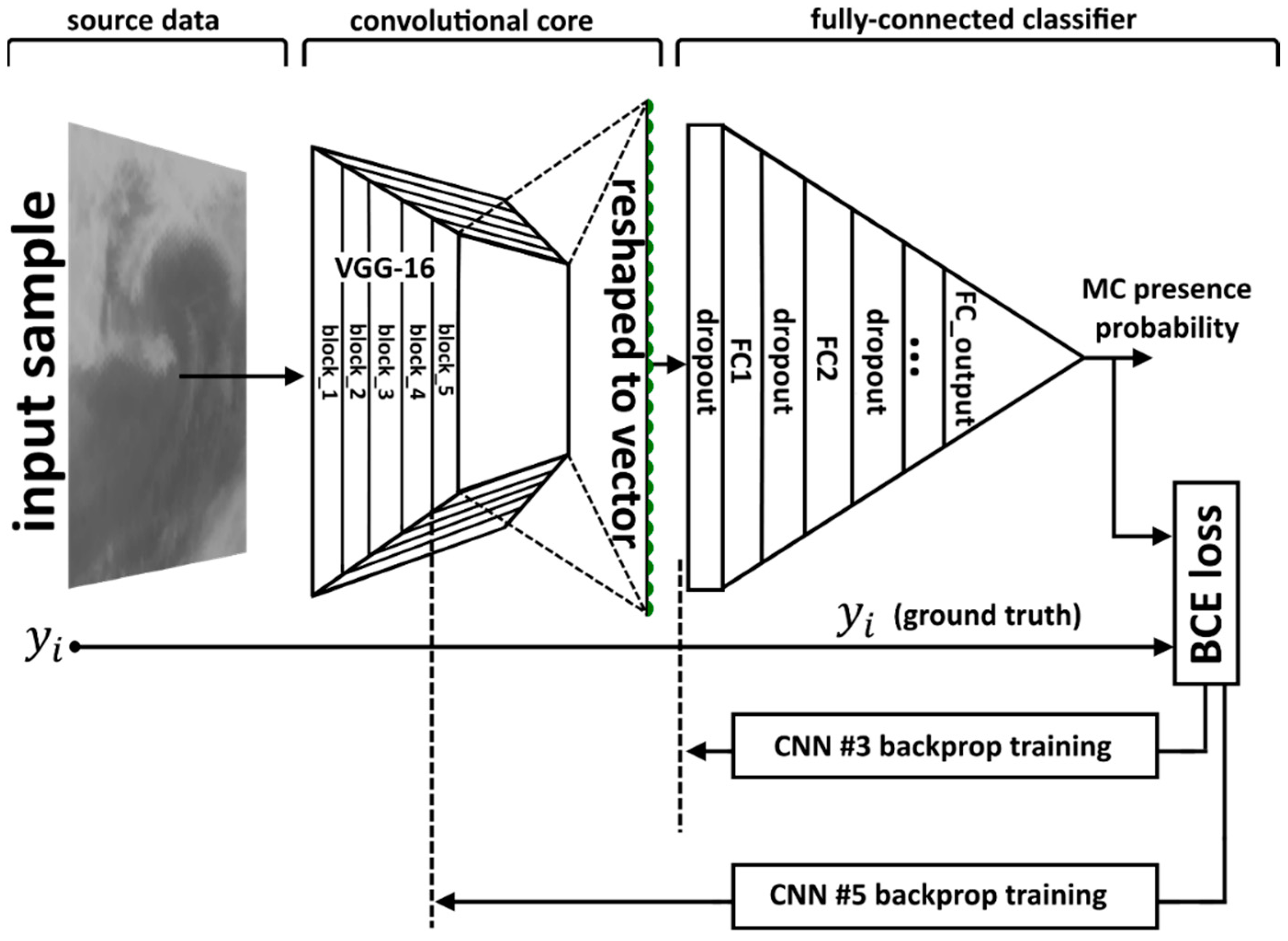
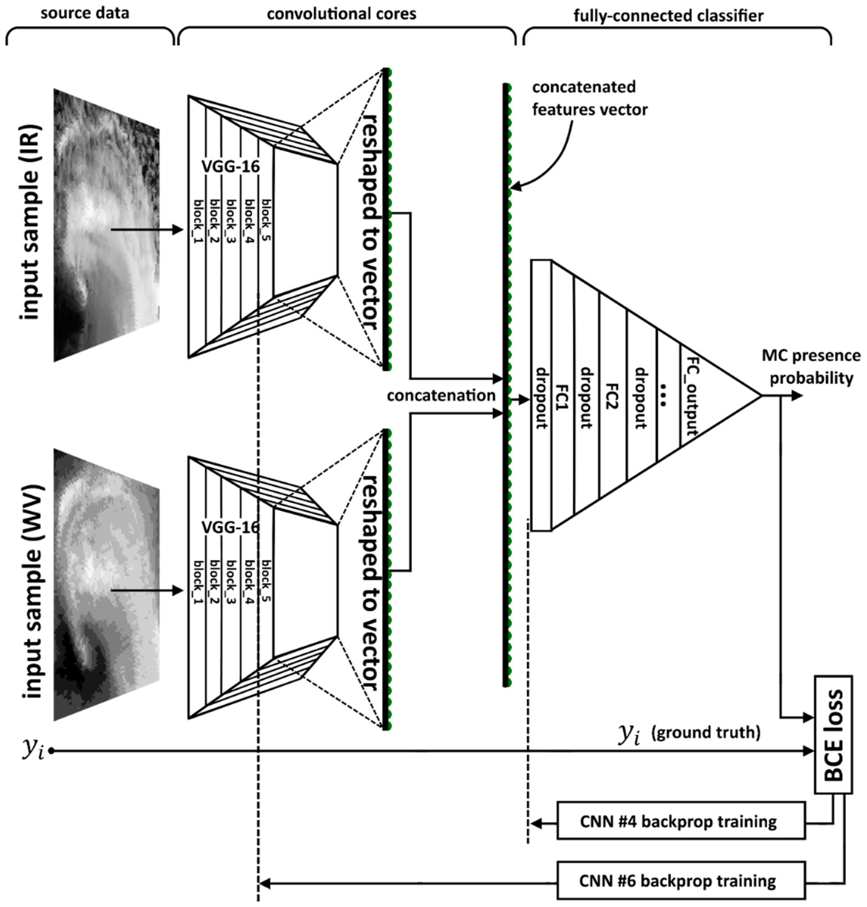
In this study, we apply the DL technique [51,52,53] to the satellite IR and WV mosaics distributed by Antarctic Meteorological Research Center [54,55]. This allows for the automated recognition of MCs cloud signatures. Our focus here is exclusively on the capability of DCNNs to perform a binary classification task regarding MCs patterns presence in patches of satellite imagery of cloudiness and/or water vapor, rather than on the DCNN-based MC tracking. This will indicate that a DCNN is capable of learning the hidden representation that is in accordance with the data and the MCs detection problem.

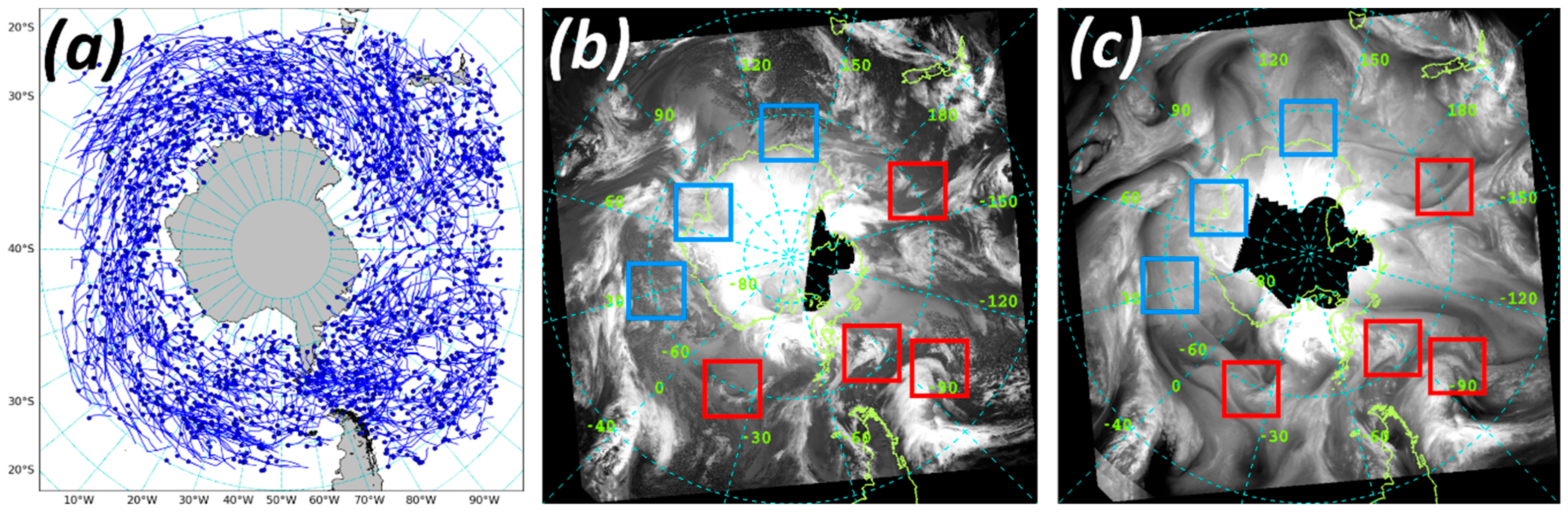
The paper is organized as follows. Section 2 describes the source data based on MC trajectories database [5]. Section 3 describes the development of the MC detection method that is based on deep convolutional neural networks and necessary data preprocessing. In Section 4, we present the results of the application of the developed methodology. Section 5 summarizes the paper with the conclusions and provides an outlook.

2. Data

For the training of DCNNs, we use the MCs dataset for the Southern Ocean (SOMC, http://sail.ocean.ru/antarctica/), consisting of 1735 MC trajectories, resulting in 9252 MC locations and associated estimates of MC sizes [5] for the four-months period (June, July, August, September) of 2004 (Figure 1a). The dataset was developed by visual identification and tracking of MCs using 976 consecutive three-hourly satellite IR (10.3–11.3 micron) and WV (~6.7 microns) mosaics provided by the Antarctic Meteorological Research Center (AMRC) Antarctic Satellite Composite Imagery (AMRC ASCI) [54,55]. These mosaics are available online (https://amrc.ssec.wisc.edu/data/) and are composites of geostationary and polar-orbiting satellite observations (GOES East and West, Meteosat, MTSAT, NOAA satellites, METOP, FY-2, Aqua, Terra etc.). This mosaics dataset is maintained by the AMRC [55]. The SOMC dataset contains longitudes and latitudes of MC centers at each three-hourly time step of the MC track, as well as MC diameter and the cloudiness signature type through the MC life cycle [5]. These characteristics were used along with the associated cloudiness patterns of MCs from the initial IR and WV mosaics for training DCNNs.

AMRC ASCI mosaics spatially combine observations from geostationary and polar-orbiting satellites and cover the area to the South of ~40° S with three-hourly temporal and 5 km spatial resolution (Figure 1b,c). While the IR channel is widely used for MCs identification [16,17,26,27,32], we also additionally employ the WV channel imagery that provides a better accuracy over the ice-covered ocean, where the IR images are potentially incorrect.

3. Methodology

3.1. Data Preprocessing

For training models, we first co-located a square (patch) of 100 × 100 mosaic pixels (500 × 500 km) with each MC center location from SOMC dataset (9252 locations in total) (Figure 2a–d). Since the distance between MCs in the multiple systems, such as the merry-go-round pattern, may be comparable to each MC diameter, and to ensure that (i) each patch covers only one MC and (ii) covers it completely, we require that MC diameters fall into 200–400 km range. Hereafter, we call this set of samples ‘the true samples’. The chosen set of true samples includes 67% of the whole population of samples in SOMC dataset.

We additionally built the set of ‘false samples’ for DCNNs training. False samples were generated from the patches that do not consist of MC-associated cloudiness signatures (Figure 2e–h) according to the SOMC dataset.

Table 1. Total number of true and false samples.

	True Samples	False Samples	Total Samples
IR	6177 (55%)	5012 (45%)	11,189 (100%)
WV	6177 (55%)	5012 (45%)	11,189 (100%)

summarizes the numbers of true and false samples that both make up the source dataset for our further analysis of IR and WV mosaics. The total number of snapshots used (both IR and WV) is 11,189. The true samples are 6177 (55%) of them, and 5012 (45%) are the false samples (see Figure 2). In order to unify images in the dataset, we normalized them by the maximum and the minimum brightness temperature (in the case of IR) over the whole dataset:

$$x_{norm}=\frac{x-\min \left(X\right)}{\max \left(X\right)-\min \left(X\right)},$$

(1)

where $x$ denotes the individual sample (represented by a matrix of 100 × 100 pixels) and $X$ is the whole dataset of 11,189 IR snapshots. The same normalization was applied to WV snapshots.

3.2. Formulation of the Problem

We consider MC identification as a binary classification problem. We use the set of true and false samples (Figure 2) as input (“objects” herein). We have developed two DCNN architectures following two conditional requirements: either (i) the object is described by the IR image only or (ii) the object is described by both IR and WV images. Since the training dataset is almost target-balanced (see Table 1), assuming ~50/50 ratio of true/false samples, we further use the accuracy score as the measure of the classification quality. The accuracy score cannot be used as a reliable quality measure of any machine learning method in the case of the unbalanced training dataset. For example, in the case of a highly unbalanced dataset with the true/false ratio being 95/5, it is easy to achieve 95% accuracy score by just forcing the model to produce only the true outcome. Thus, balancing the source dataset with false samples is critical for building the reliable classification model.

3.3. Justification of Using DCNN

There is a set of best practices commonly used to construct DCNNs for solving classification problems [56]. While building and training DCNNs for MCs identifications, we applied the technique that was proposed by LeCun [41]. This technique implies the usage of consecutive convolutional layers that detect spatial data patterns, alternating with subsampling layers, which reduce the sample dimensions. The set of these layers is followed by a set of so-called fully-connected (FC) layers representing a neural classifier. The whole model built in this manner represents a non-linear classifier that is capable of directly predicting a target value for the input sample. A very detailed description of this model architecture can be found in [41]. We will further term the FC layers set as “FC classifier”, and the preceding part containing convolutional and pooling layers as “convolutional core” (see Figure 3 and Figure 4). The outcome of the whole model is the probability of MC presence in the input sample.

While handling multiple concurrent and spatially aligned geophysical fields, it is important to choose a suitable approach. LeCun [41] proposed the DCNN focused on the processing of only grayscale images—meaning just one 2D field. In order to handle multiple 2D fields, they may be stacked together to form a three-dimensional (3D) matrix by analogy with colorful images which have three color channels: red, green and blue. This approach can be applied when one uses pre-trained networks like AlexNet [36], VGG16 [45], ResNet [48] or similar architectures because of the original purpose of these networks to classify colorful images. However, this approach should be exploited carefully when applied to geophysical fields, because the mentioned networks were trained using massive datasets (e.g., ImageNet) of real photographed scenes, which means specific dependencies laying between channels (red, green and blue) within each image. In contrast to the stacking approach applied by Liu et al. [39], we use separate CNN branch for each channel (IR and WV) to ensure that we are not limiting the overall quality of the whole network (see Figure 4). In the following, we describe in detail each DCNN architecture for both cases: IR + WV (Figure 4) and IR alone (Figure 3).

Since we consider the binary classification, and the source dataset is almost target-balanced (see Table 1), we use as a quality measure the accuracy score or $Acc$, which is a rate of objects, classified correctly as compared to the ground truth:

$$Acc=\frac{1}{\parallel \mathcal{T}\parallel }{\displaystyle \sum }_{\mathcal{T}}\left[\widehat{y_i}=y_i\right],$$

(2)

where $\mathcal{T}$ denotes the dataset and $\parallel \mathcal{T}\parallel$ is its total samples count; $y_i$ is expert-defined target value (ground truth), $\widehat{y_i}$ is the model decision whether the $i$-th object contain MC.

In addition to the baseline that is the network proposed in [41], we applied a set of additional approaches that are commonly used to improve the DCNN accuracy and generalization ability (see Appendix A). Specifically, we used Transfer Learning (TL) [57,58,59,60,61,62] with the VGG16 [45] network pre-trained on ImageNet [49] dataset; Fine Tuning (FT) [63], Dropout (Do) [64], and dataset augmentation (DA) [65] (see Appendix A). With these techniques applied in various combinations, we constructed six DCNN architectures that are summarized in

Table 2. Accuracy score of each model with the best hyper-parameters combination. BA—basic approach [41], TL—Transfer Learning, FT—Fine Tuning, Do—dropout, DA—dataset augmentation. $Acc$ is the accuracy score averaged across models of the particular architecture. AsEA is the accuracy score of the ensemble averaged models with the optimal probability threshold. $p_{th}$ is the optimal probability threshold value.

Model Name	IR	WV	BA	TL	FT	Do	DA	$\mathit{A}\mathit{c}\mathit{c}$	AsEA	${\mathit{p}}_{\mathit{t}\mathit{h}}$
CNN #1	X	-	X	-	-	X	X	86.89 ± 1.1%	89.3%	0.381
CNN #2	X	X	X	-	-	X	X	94.1 ± 1.4%	96.3%	0.272
CNN #3	X	-	X	X	-	X	X	95.8 ± 0.1%	96.6%	0.556
CNN #4	X	X	X	X	-	X	X	95.5 ± 0.3%	96.3%	0.526
CNN #5	X	-	X	X	X	X	X	96 ± 0.2%	96.6%	0.5715
CNN #6	X	X	X	X	X	X	X	95.7 ± 0.2%	96.4%	0.656
Third-order model CNN #1–6 averaged ensemble									97%	0.598

. All of these architectures are built in a common manner: the FC classifier follows the one- (for IR only) or two-branched (for IR + WV) convolutional core. If the convolutional core is one-branched, its output itself is input data for the corresponding FC classifier. If the convolutional core is two-branched, the concatenation product of their outputs is the input data for the corresponding FC classifier. The very detailed description of the constructed architectures is presented in Appendix A. For each DCNN structure, we trained a set of models, as described in detail in Section 3.5. We also applied ensemble averaging (see Appendix A) of a set of models of identical configuration via averaging probabilities of true class for each object of the dataset. We term these six ensemble-averaged models the “second-order” models. We also applied ensemble averaging per sample of all trained DCNNs that were trained in this work. We term this model the “third-order” model. Each of these models was trained using the method of backpropagation of error (BCE loss, see Appendix A) [66], denoted as “backprop training” in Figure 3 and Figure 4.

3.4. Proposed DCNN Architectures

Six DCNNs that we have constructed are able to perform binary classification on satellite mosaics data (IR alone or IR + WV) represented as grayscale 100 × 100 pixels images:

• CNN #1. This model is built “from scratch” which means we have not used any pre-trained networks. CNN #1 is built in the manner proposed in [35]. We varied sizes of convolutional kernels of each convolutional layers from 3 × 3 to 5 × 5. We also varied sizes of subsampling layers’ receptive fields from 2 × 2 to 3 × 3. For each convolutional layer, we varied the number of convolutional kernels: 8, 16, 32, 64 and 100. The network convolutional core consists of three convolutional layers alternated with subsampling layers. Each pair of convolutional and subsampling layers is followed by a dropout layer. CNN #1 is one-branched, and objects are described by IR 500 × 500 km satellite snapshots only.
• CNN #2. This model is built “from scratch” with two separate branches-for IR and WV data. The convolutional core of each branch is built in the same manner as the convolutional core for CNN #1 and as proposed in [41]. We varied the same parameters of the structure here in the same ranges as for CNN #1.
• CNN #3. This model is built with TL approach. We used VGG16 pre-trained convolutional core to construct this model. None of VGG16 weights were optimized within this model, and only the weights of the FC classifier were trainable. This model is one-branched, and the objects are described by IR 500 × 500 km satellite snapshots only. CNN #3 structure is shown in Figure 3.
• CNN #4. This model is two-branched, and each branch of its convolutional core is built with TL approach, in the same manner as the convolutional core of CNN #3. Input data are IR and WV. None of VGG16 weights of this model in any of the two branches were optimized, and only the weights of the FC classifier were trainable. CNN #4 structure is shown in Figure 4.
• CNN #5 is built with both TL and FT approaches. We built the convolutional core of this model with the use of VGG16 pre-trained network. VGG16 convolutional core consists of five similar blocks of layers. For the CNN #5 we turned the last of these five blocks to be trainable. This model is one-branched, and objects are IR 500 × 500 km satellite snapshots only. CNN #5 structure is shown in Figure 3.
• CNN #6 is two-branched, and branches of its convolutional core are built in the same manner as the convolutional core of CNN #5. For the CNN #6, we turned the last of five blocks of each VGG16 convolutional cores to be trainable. Input data are IR and WV 500 × 500 km satellite snapshots of dataset samples. CNN #6 structure is shown in Figure 4.

3.5. Computational Experiment Design

The following hyper-parameters are included in each of the six networks:

• Size (number of nodes) of the first layer of FC classifier (denoted as FC1 in Figure 3 and Figure 4)
• Convolutional kernels count for each convolutional layer (only applies to CNN #1 and CNN #2)
• Sizes of convolutional kernels (only applies to CNN #1 and CNN #2)
• Sizes of receptive fields of subsampling layers (only applies to CNN #1 and CNN #2)

The whole dataset was split into training (8952 samples) and testing (2237 samples) sets stratified by target value meaning that each set has the same (55:45) ratio of true/false samples as the whole dataset (i.e., 4924:4028 and 1253:984 samples in training and testing sets correspondingly). We have conducted hyper-parameters optimization for each of these DCNNs using stratified K-fold (K = 5) cross-validation approach. After this optimization, we trained several (typically 14–18) models with the best hyper-parameters configuration on the training set for each architecture (architecture-specific models). Then, we excluded models with the maximal and minimal accuracy score being estimated with the cross-validation approach, from this set of architecture-specific models for each of the six architectures. The remaining architecture-specific models were evaluated on the testing set, which was never seen by these models. We estimated the accuracy score for each individual model and the variance of accuracy score for the particular architecture with the best hyper-parameters combination (see Table 2).

With the ensemble averaging approach, we evaluated the second-order models on the “never-seen by the model” testing set. As described in Section 3.3, we estimated the optimal probability threshold $p_{th}$ for each second-order model and for the third-order model (see Table 2) for the best accuracy score estimation. These scores are treated as the quality measure of each particular architecture.

Numerical optimization and evaluation of models were performed at the Data Center of Far Eastern Branch of Russian Academy of Sciences (FEB RAS) [67] and DL computational resources of Sea-Air Interactions Laboratory of Shirshov Institute of Oceanology of Russian Academy of Sciences (IORAS, https://sail.ocean.ru/). Exploited computational nodes contain two graphics processing units (GPU) NVIDIA Tesla P100 16GB RAM. With these resources, the total GPU time of calculations is 3792 h.

4. Results

The designed DCNNs were applied to detect of Antarctic MCs for the period from June to September 2004. Summary of the results of the application of six models is presented in Table 2. As we noted above, each model is characterized by the utilized data source (IR alone or IR + WV, columns “IR” and “WV” in Table 2). These DCNNs are further categorized according to a chosen set of applied techniques in addition to the basic approach (see Table 2 legend). Table 2 also provides accuracy scores and probability thresholds estimated, as described in Section 3.5, for the individual, second-, and third-order models of each architecture.

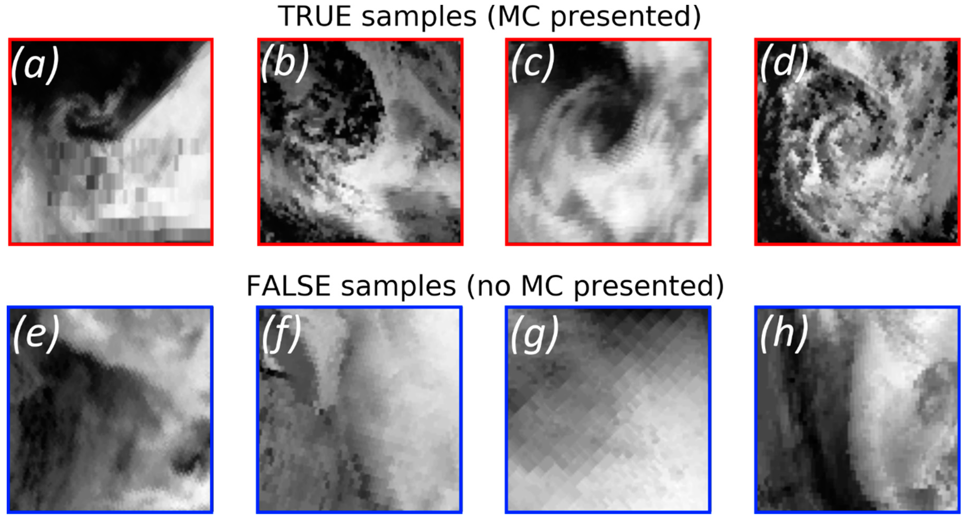
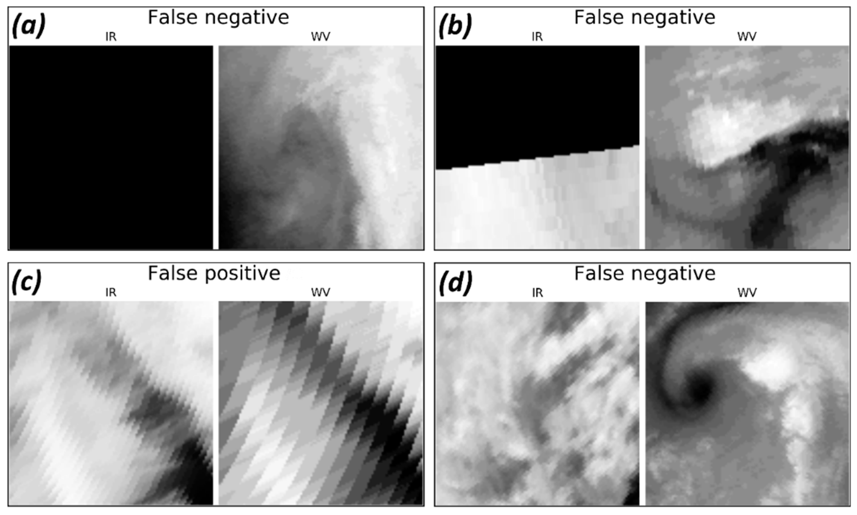
Figure 5 demonstrates four main types of false classified objects. The first and the second types are the ones for which IR data are missing completely or partially. The third type is the one for which the source satellite data were suspected to be corrupted. These three types of classifier errors originating from the lack of source data or the corruption of source data. For the fourth type, the source satellite data were realistic but the classifier has made a mistake. Thus, some of false classifications are model mistakes, and some are associated with the labeling issue where human expert could guess on the MC propagation over the area with missing or corrupted satellite data.

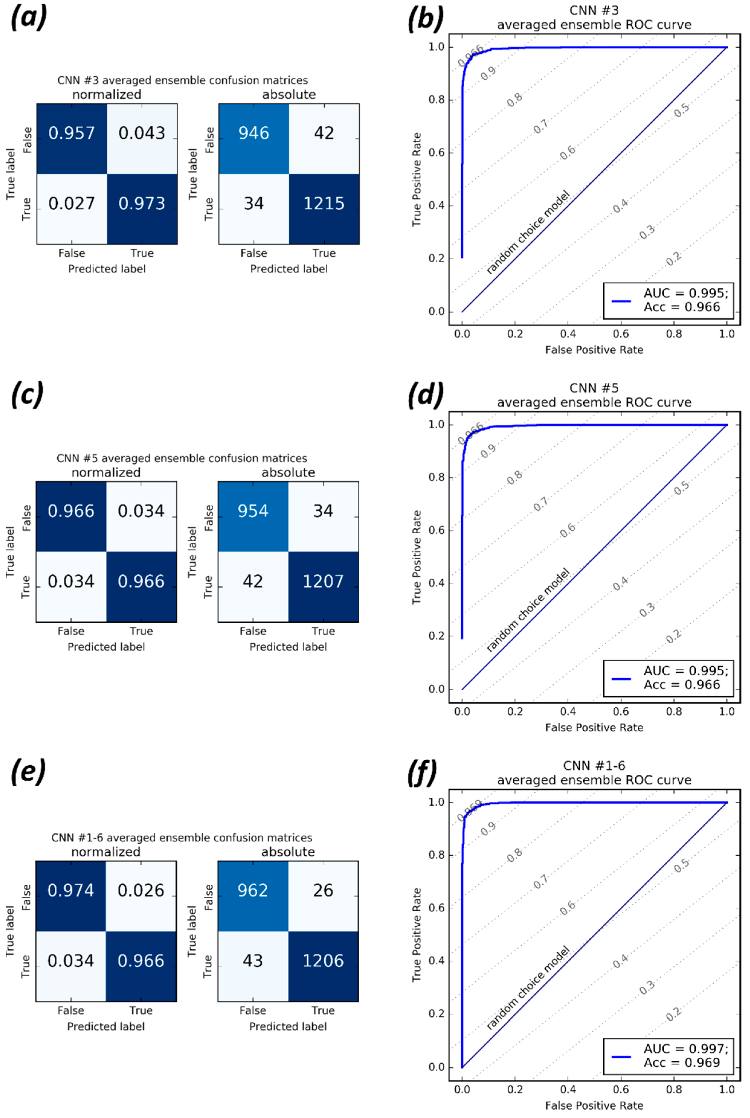
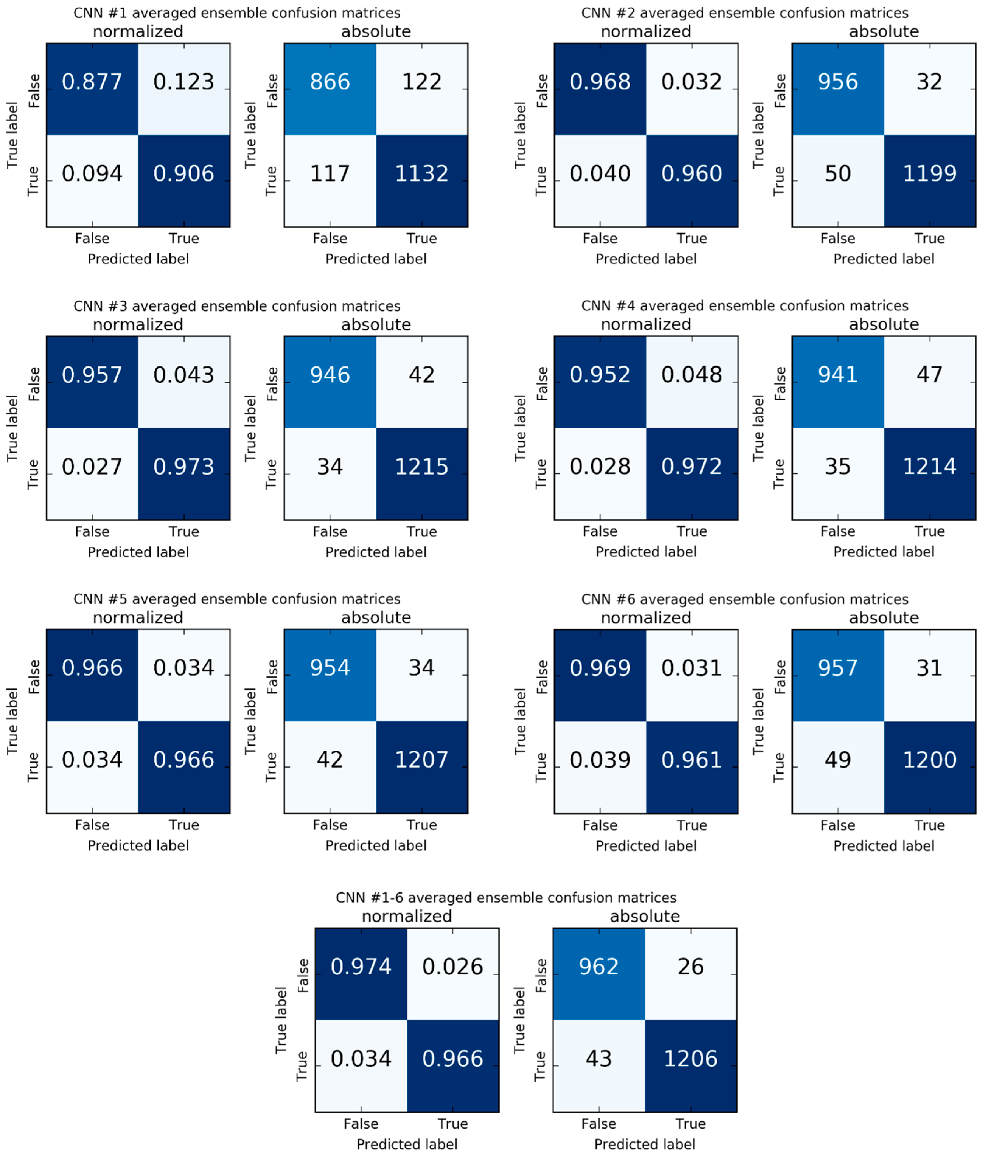
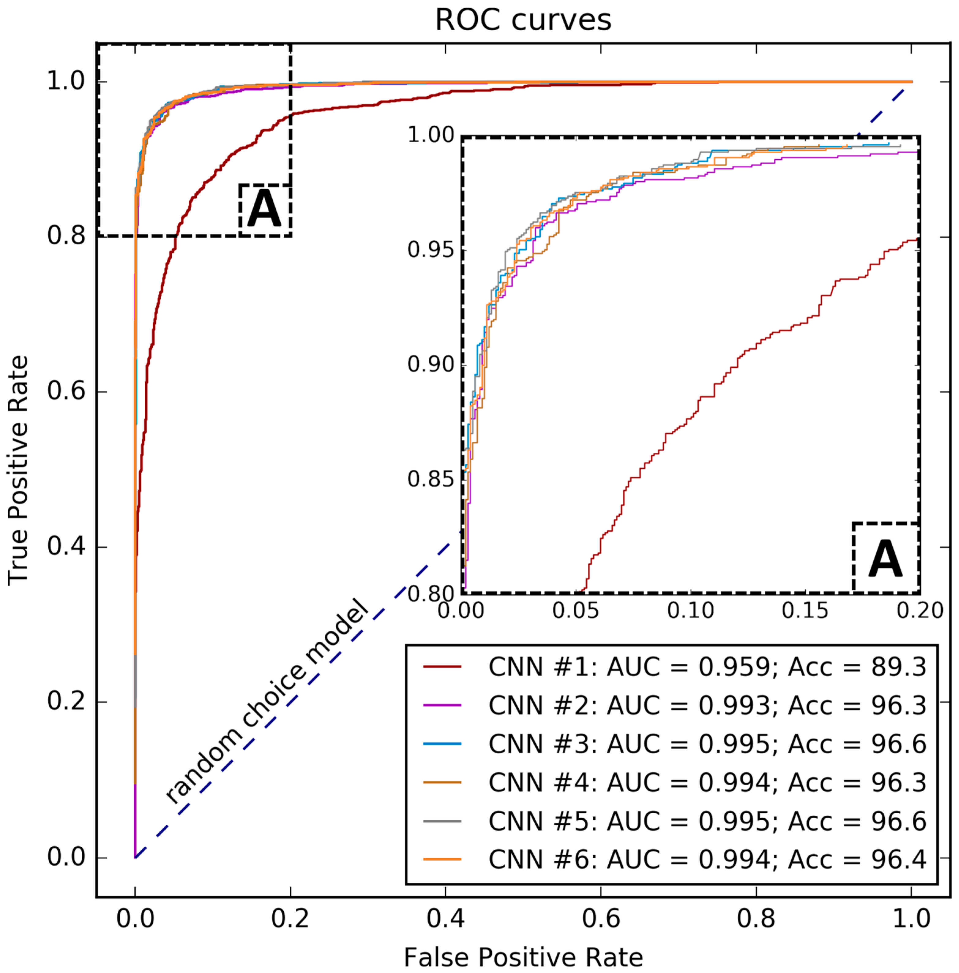
As shown in Table 2, CNN #3 and CNN #5 demonstrated the best accuracy among the second-order models on a never-seen subset of objects. The best combination of hyper-parameters for these networks is presented in Appendix B. Confusion matrices and receiver operating characteristic (ROC) curves for these models are shown in Figure 6a–d. Confusion matrices and ROC curves for all evaluated models are presented in Appendix C. Figure 6 clearly confirms that these two models perform almost equally for the true and the false samples. According to Table 2, the best accuracy score is reached using different probability thresholds for each second- or third-order model.

Comparison of CNN #1, CNN #2, on the one hand, and the remaining models, on the other hand, shows that DCNNs built with the use of TL technique demonstrate better performance when compared to the models built “from scratch”. Moreover, the accuracy score variances of CNN #1 and CNN #2 are higher than for the other architectures. Thus, models built with TL approach seem to be more stable, and their generalization ability is better, as compared to models built “from scratch”.

Comparing CNN #1 and CNN #2 qualities, we may conclude that the use of an additional data source (WV) results in the significant increase of the model accuracy score. Comparison of models within each pair of the network configurations (CNN #3 vs. CNN #5; CNN #4 vs. CNN #6) demonstrates that the FT approach does not provide significant improvement of the accuracy score in case of such a small size of the dataset. It is also obvious that the averaging over the ensemble members does increase the accuracy score from 0.6% for CNN #5 to 2.41% for CNN #1. However, in some cases, these score increases are comparable to the corresponding accuracy standard deviations.

It is also clear from the last row of Table 2, that the third-order model, which averages probabilities that are estimated by all trained models CNN #1–6, produces the accuracy of $Acc=97\%$ which outperforms all scores of individual models and second-order ensemble models. ROC curve and confusion matrices for this model are presented in Figure 6e,f.

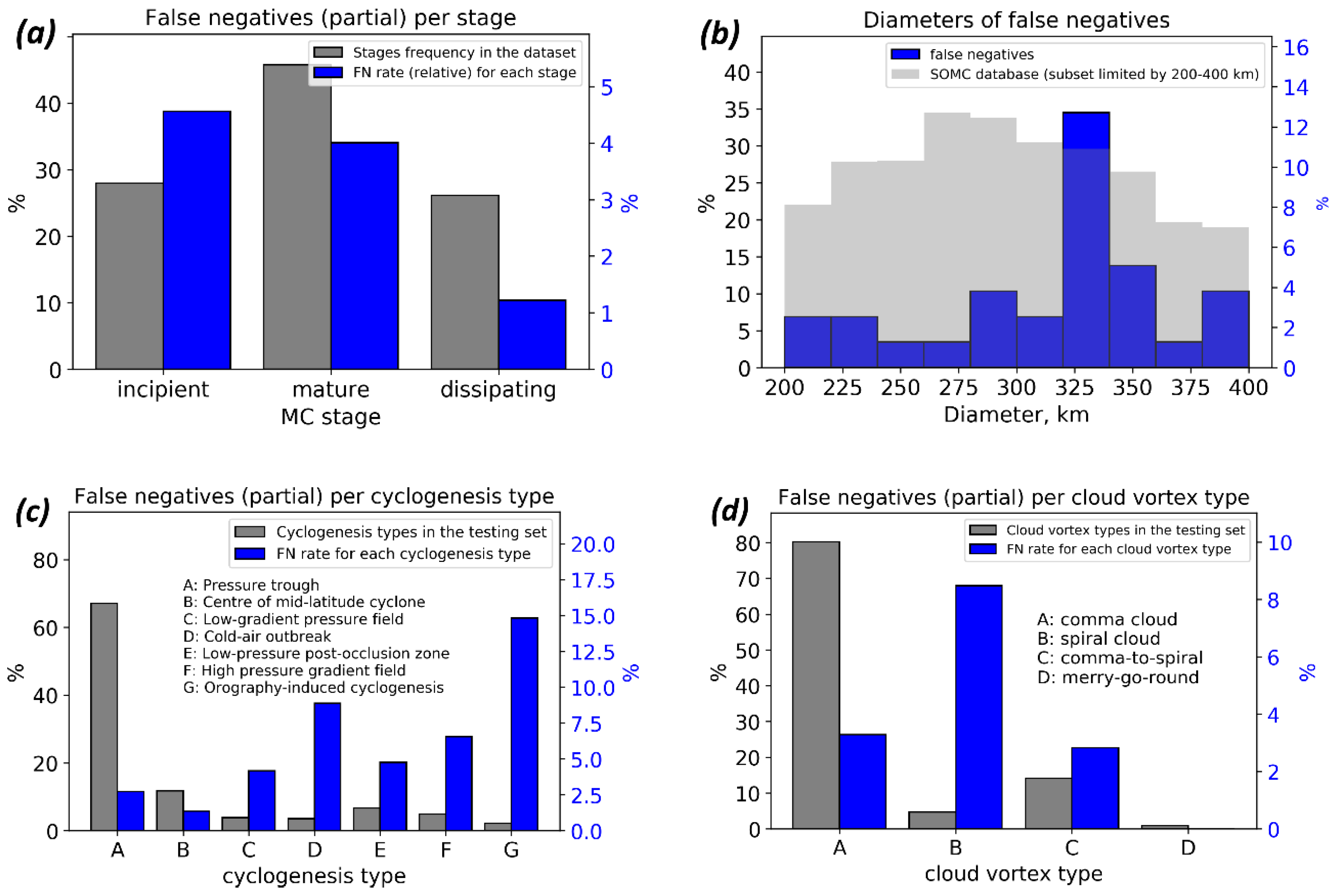
Figure 7 demonstrates the characteristics of the best model (third-order ensemble-averaging model) regarding false negatives (FN). Since the testing set is unbalanced with respect to stages, types of cyclogenesis and cloud vortex types, which we present in Figure 7a,c,d relative FN rates for each separate class in each taxonomy. We present the testing set distribution of classes for these taxonomies as well. Note that scales are different for reference distributions of classes of the testing set and the distributions of missed MCs. Detailed false negatives characteristics may be found in Appendix D.

Tracking procedure requires the sustainable ability of the MCs detection scheme to recognize mesocyclone cloud shape imprints during the whole MC life cycle. Figure 7a demonstrates that the best model classifies mesocyclone imprints almost equally for incipient (~4.6% incipient missed) and mature (~4% mature missed) stages. The fraction of missed MCs in its dissipating stage is lower (~4% missed among MCs in dissipating stage). As for distribution of missed MCs with respect to their diameters (see Figure 7b), the histogram demonstrates fractions of FN objects relative to the whole FN number. The distribution of MC diameters in the testing set in Figure 7b is shown as a reference. There is a peak around the diameter value of 325 km, which does not coincide with any issues of distributions of MC diameters when the testing set is subset by any particular class of any taxonomy. However, since the total number of missed MCs is too small, there is no obvious reason to make assumptions on the origin of this issue. The FN rates per cyclogenesis types (Figure 7c) demonstrate the only issue for the orography-induced MCs. This issue is caused by the total number of that cyclogenesis type, which is small (only 27 MCs in the testing set and only 134 in the training set), so the four that were missed is a substantial fraction of it. The same issue is demonstrated for the FN rates per cloud vortex types. Since the total number of “spiral cloud” type in the testing set is relatively small (59 of 1253), the five missed are a substantial fraction of it, as compared to 33 missed of 1006 for “comma cloud” type.

5. Conclusions and Outlook

In this study, we present an adaptation of a DCNN method resulting in an algorithm that recognizes MCs signatures in preselected patches of satellite imagery of cloudiness and spatially collocated WV imagery. The DCNN technique shows very high accuracy in this problem. The best accuracy score of 97% is reached using the third-order ensemble-averaging model (six models ensemble) and the combination of both IR and WV images as input. We assess the accuracy of MCs recognition by comparison of identified MCs (true/false—image contain MC/no MC on the image parameter) with a reference dataset [5]. We demonstrate that deep convolutional networks are capable of effectively detecting the presence of polar mesocyclone signatures in satellite imagery patches of size 500 × 500 km. We also conclude that the quality of the satellite mosaics is sufficient enough for performing the task of binary classification regarding the MCs presence in 500 × 500 km patches, and for performing other similar tasks of pattern recognition type, e.g., semantic segmentation of MCs.

Since the satellite-based studies of polar mesocyclone activity conducted in the SH (and in NH as well) have never reported season-dependent variations of IR imprint of cloud shapes of MCs [23,27,68,69], we assume the proposed methodology to be applicable to satellite imageries of polar MCs that are available for the whole satellite observation era in SH. In the NH, the direct application of the models that were trained on SH dataset is restricted due to the opposite sign of relative vorticity, and thus, different cloud shape orientation. However the proposed approach is still applicable, and the only need is a dataset of tracks of MCs from the NH.

It was also shown that the accuracy of MCs detection by DCNNs is sensitive to the single (IR only) or double (IR + WV) input data usage. IR+WV combination provides significant improvement of the detection of MCs and allows a weak DCNN (CNN #2) to detect MCs with higher accuracy compared to the weak CNN #1 (89.3% and 96.3% correspondingly). The computational cost of DCNN training and hyper-parameters optimization for deep neural networks are time- and computational-consuming. However, once trained, the computational cost of the DCNN inference is low. Furthermore, the trained DCNN performs much faster when compared to a human expert. Another advantage of the proposed method is the low computational cost of data preprocessing that allows the processing of satellite imagery in real time or the processing of large amounts of collected satellite data.

We plan to extend the usage of this set of DCNNs (Table 2) for the development of an MCs tracking method based on machine learning and using satellite IR and WV mosaics. These efforts would be mainly focused on the development of the optimal choice of the “cut-off” window that has to be applied to the satellite mosaic. In the case of a sliding-window approach (e.g., running the 500 × 500 km sliding window through the mosaics), the virtual testing dataset of the whole mosaic is highly unbalanced, so a model with non-zero FPR evaluated on balanced dataset would produce much higher FPR. Thus, we expect the sliding-window approach not to be accurate enough in the problem of MC detection. In the future, instead of the sliding-window, the Unet-like [70,71] architecture should be considered with the binary semantic segmentation problem formulation. Since the models that have been applied in this study (specifically their convolutional cores) are capable of extracting the hidden representation that is relevant to MCs signatures, they may be used as the encoder part of the Unet-like encoder-decoder neural network for MCs identification and tracking. Considering MC tracking development, an approach proposed in a number of face recognition studies should be reassuring [72,73]. This approach can be applied in a manner of triple-based training of the DCNN to estimate a measure of similarity between one particular MC signatures in consecutive satellite mosaics.

References

1. Thorpe, A.J. Polar Lows: Mesoscale Weather Systems in the Polar Regions; Rasmussen, E.A., Turner, J., Eds.; Cambridge University Press: Cambridge, UK, 2003; ISBN 978-0-511-52497-4. [Google Scholar]
2. Marshall, J.; Schott, F. Open-ocean convection: Observations, theory, and models. Rev. Geophys. 1999, 37, 1–64. [Google Scholar] [CrossRef] [Green Version]
3. Condron, A.; Renfrew, I.A. The impact of polar mesoscale storms on northeast Atlantic Ocean circulation. Nat. Geosci. 2013, 6, 34–37. [Google Scholar] [CrossRef]
4. Condron, A.; Bigg, G.R.; Renfrew, I.A. Modeling the impact of polar mesocyclones on ocean circulation. J. Geophys. Res. Oceans 2008, 113. [Google Scholar] [CrossRef] [Green Version]
5. Verezemskaya, P.; Tilinina, N.; Gulev, S.; Renfrew, I.A.; Lazzara, M. Southern Ocean mesocyclones and polar lows from manually tracked satellite mosaics. Geophys. Res. Lett. 2017, 44, 7985–7993. [Google Scholar] [CrossRef]
6. Laffineur, T.; Claud, C.; Chaboureau, J.-P.; Noer, G. Polar lows over the Nordic Seas: Improved Representation in ERA-Interim Compared to ERA-40 and the Impact on Downscaled Simulations. Mon. Weather Rev. 2014, 142, 2271–2289. [Google Scholar] [CrossRef]
7. Michel, C.; Terpstra, A.; Spengler, T. Polar Mesoscale Cyclone Climatology for the Nordic Seas Based on ERA-Interim. J. Clim. 2017, 31, 2511–2532. [Google Scholar] [CrossRef]
8. Bromwich, D.H.; Wilson, A.B.; Bai, L.-S.; Moore, G.W.K.; Bauer, P. A comparison of the regional Arctic System Reanalysis and the global ERA-Interim Reanalysis for the Arctic. Q. J. R. Meteorol. Soc. 2016, 142, 644–658. [Google Scholar] [CrossRef]
9. Press, W.H.; Teukolsky, S.A.; Vetterling, W.T.; Flannery, B.P. Numerical Recipes 3rd Edition: The Art of Scientific Computing; Cambridge University Press: Cambridge, UK, 2007; ISBN 0-521-88068-8. [Google Scholar]
10. Rojo, M.; Claud, C.; Mallet, P.-E.; Noer, G.; Carleton, A.M.; Vicomte, M. Polar low tracks over the Nordic Seas: A 14-winter climatic analysis. Tellus A Dyn. Meteorol. Oceanogr. 2015, 67, 24660. [Google Scholar] [CrossRef]
11. Smirnova, J.; Golubkin, P. Comparing Polar Lows in Atmospheric Reanalyses: Arctic System Reanalysis versus ERA-Interim. Mon. Weather Rev. 2017, 145, 2375–2383. [Google Scholar] [CrossRef]
12. Hines, K.M.; Bromwich, D.H. Development and Testing of Polar Weather Research and Forecasting (WRF) Model. Part I: Greenland Ice Sheet Meteorology. Mon. Weather Rev. 2008, 136, 1971–1989. [Google Scholar] [CrossRef]
13. Zappa, G.; Shaffrey, L.; Hodges, K. Can Polar Lows be Objectively Identified and Tracked in the ECMWF Operational Analysis and the ERA-Interim Reanalysis? Mon. Weather Rev. 2014, 142, 2596–2608. [Google Scholar] [CrossRef]
14. Pezza, A.; Sadler, K.; Uotila, P.; Vihma, T.; Mesquita, M.D.S.; Reid, P. Southern Hemisphere strong polar mesoscale cyclones in high-resolution datasets. Clim. Dyn. 2016, 47, 1647–1660. [Google Scholar] [CrossRef]
15. Xia, L.; Zahn, M.; Hodges, K.; Feser, F.; Storch, H. A comparison of two identification and tracking methods for polar lows. Tellus A Dyn. Meteorol. Oceanogr. 2012, 64, 17196. [Google Scholar] [CrossRef]
16. Harold, J.M.; Bigg, G.R.; Turner, J. Mesocyclone activity over the North-East Atlantic. Part 1: Vortex distribution and variability. Int. J. Climatol. 1999, 19, 1187–1204. [Google Scholar] [CrossRef]
17. Noer, G.; Saetra, Ø.; Lien, T.; Gusdal, Y. A climatological study of polar lows in the Nordic Seas. Q. J. R. Meteorol. Soc. 2011, 137, 1762–1772. [Google Scholar] [CrossRef] [Green Version]
18. Smirnova, J.E.; Zabolotskikh, E.V.; Bobylev, L.P.; Chapron, B. Statistical characteristics of polar lows over the Nordic Seas based on satellite passive microwave data. Izv. Atmos. Ocean. Phys. 2016, 52, 1128–1136. [Google Scholar] [CrossRef]
19. McMurdie, L.A.; Claud, C.; Atakturk, S. Satellite-derived atmospheric characteristics of spiral and comma-shaped southern hemisphere mesocyclones. J. Geophys. Res. Atmos. 1997, 102, 13889–13905. [Google Scholar] [CrossRef] [Green Version]
20. Irving, D.; Simmonds, I.; Keay, K. Mesoscale Cyclone Activity over the Ice-Free Southern Ocean: 1999–2008. J. Clim. 2010, 23, 5404–5420. [Google Scholar] [CrossRef]
21. Neu, U.; Akperov, M.G.; Bellenbaum, N.; Benestad, R.; Blender, R.; Caballero, R.; Cocozza, A.; Dacre, H.F.; Feng, Y.; Fraedrich, K.; et al. IMILAST: A Community Effort to Intercompare Extratropical Cyclone Detection and Tracking Algorithms. Bull. Am. Meteorol. Soc. 2013, 94, 529–547. [Google Scholar] [CrossRef]
22. Wilhelmsen, K. Climatological study of gale-producing polar lows near Norway. Tellus A Dyn. Meteorol. Oceanogr. 1985, 37, 451–459. [Google Scholar] [CrossRef]
23. Carrasco, J.F.; Bromwich, D.H. Mesoscale cyclogenesis dynamics over the southwestern Ross Sea, Antarctica. J. Geophys. Res. Atmos. 1993, 98, 12973–12995. [Google Scholar] [CrossRef]
24. Carrasco, J.F.; Bromwich, D.H.; Liu, Z. Mesoscale cyclone activity over Antarctica during 1991: 1. Marie Byrd Land. J. Geophys. Res. Atmos. 1997, 102, 13923–13937. [Google Scholar] [CrossRef] [Green Version]
25. Turner, J.; Thomas, J.P. Summer-season mesoscale cyclones in the bellingshausen-weddell region of the antarctic and links with the synoptic-scale environment. Int. J. Climatol. 1994, 14, 871–894. [Google Scholar] [CrossRef]
26. Harold, J.M.; Bigg, G.R.; Turner, J. Mesocyclone activity over the Northeast Atlantic. Part 2: An investigation of causal mechanisms. Int. J. Climatol. 1999, 19, 1283–1299. [Google Scholar] [CrossRef] [Green Version]
27. Carleton, A.M. On the interpretation and classification of mesoscale cyclones from satellite infrared imagery. Int. J. Remote Sens. 1995, 16, 2457–2485. [Google Scholar] [CrossRef]
28. Claud, C.; Katsaros, K.B.; Mognard, N.M.; Scott, N.A. Comparative satellite study of mesoscale disturbances in polar regions. Glob. Atmos. Ocean Syst. 1996, 4, 233–273. [Google Scholar]
29. Gang, F.; Qin-yu, L.; Zeng-mao, W. General features of polar lows over the Japan Sea and the Northwestern Pacific. Chin. J. Ocean. Limnol. 1999, 17, 300–307. [Google Scholar] [CrossRef]
30. Gurvich, I.A.; Pichugin, M.K. Study of the compara tive characteristics of typical mesoscale cyclones over Far Eastern seas on the basis of satellite multisensory sounding. Sovrem. Probl. Distantsionnogo Zondirovaniya Zemli Kosmosa 2013, 10, 51–59. [Google Scholar]
31. Claud, C.; Carleton, A.M.; Duchiron, B.; Terray, P. Southern hemisphere winter cold-air mesocyclones: Climatic environments and associations with teleconnections. Clim. Dyn. 2009, 33, 383–408. [Google Scholar] [CrossRef]
32. Blechschmidt, A.-M. A 2-year climatology of polar low events over the Nordic Seas from satellite remote sensing. Geophys. Res. Lett. 2008, 35. [Google Scholar] [CrossRef] [Green Version]
33. Heinle, A.; Macke, A.; Srivastav, A. Automatic cloud classification of whole sky images. Atmos. Meas. Tech. 2010, 3, 557–567. [Google Scholar] [CrossRef] [Green Version]
34. Taravat, A.; Frate, F.D.; Cornaro, C.; Vergari, S. Neural Networks and Support Vector Machine Algorithms for Automatic Cloud Classification of Whole-Sky Ground-Based Images. IEEE Geosci. Remote Sens. Lett. 2015, 12, 666–670. [Google Scholar] [CrossRef]
35. Onishi, R.; Sugiyama, D. Deep Convolutional Neural Network for Cloud Coverage Estimation from Snapshot Camera Images. SOLA 2017, 13, 235–239. [Google Scholar] [CrossRef] [Green Version]
36. Krizhevsky, A.; Sutskever, I.; Hinton, G.E. Imagenet classification with deep convolutional neural networks. In Advances in Neural Information Processing Systems; MIT Press: Cambridge, MA, USA, 2012; pp. 1097–1105. [Google Scholar]
37. Shin, H.-C.; Roth, H.R.; Gao, M.; Lu, L.; Xu, Z.; Nogues, I.; Yao, J.; Mollura, D.; Summers, R.M. Deep Convolutional Neural Networks for Computer-Aided Detection: CNN Architectures, Dataset Characteristics and Transfer Learning. IEEE Trans. Med. Imaging 2016, 35, 1285–1298. [Google Scholar] [CrossRef] [PubMed]
38. Krinitskiy, M.A. Application of machine learning methods to the solar disk state detection by all-sky images over the ocean. Oceanology 2017, 57, 265–269. [Google Scholar] [CrossRef]
39. Liu, Y.; Racah, E.; Correa, J.; Khosrowshahi, A.; Lavers, D.; Kunkel, K.; Wehner, M.; Collins, W. Application of deep convolutional neural networks for detecting extreme weather in climate datasets. arXiv, 2016; arXiv:1605.01156. [Google Scholar]
40. Huang, D.; Du, Y.; He, Q.; Song, W.; Liotta, A. DeepEddy: A simple deep architecture for mesoscale oceanic eddy detection in SAR images. In Proceedings of the 2017 IEEE 14th International Conference on Networking, Sensing and Control (ICNSC), Calabria, Italy, 16–18 May 2017; pp. 673–678. [Google Scholar]
41. Lecun, Y.; Bottou, L.; Bengio, Y.; Haffner, P. Gradient-based learning applied to document recognition. Proc. IEEE 1998, 86, 2278–2324. [Google Scholar] [CrossRef] [Green Version]
42. LeCun, Y.; Bengio, Y.; Hinton, G. Deep learning. Nature 2015, 521, 436–444. [Google Scholar] [CrossRef] [PubMed]
43. Liu, W.; Wang, Z.; Liu, X.; Zeng, N.; Liu, Y.; Alsaadi, F.E. A survey of deep neural network architectures and their applications. Neurocomputing 2017, 234, 11–26. [Google Scholar] [CrossRef]
44. Guo, Y.; Liu, Y.; Oerlemans, A.; Lao, S.; Wu, S.; Lew, M.S. Deep learning for visual understanding: A review. Neurocomputing 2016, 187, 27–48. [Google Scholar] [CrossRef]
45. Simonyan, K.; Zisserman, A. Very Deep Convolutional Networks for Large-Scale Image Recognition. arXiv, 2014; arXiv:1409.1556. [Google Scholar]
46. Szegedy, C.; Liu, W.; Jia, Y.; Sermanet, P.; Reed, S.; Anguelov, D.; Erhan, D.; Vanhoucke, V.; Rabinovich, A. Going deeper with convolutions. In Proceedings of the IEEE Conference on Computer Vision and Pattern Recognition (CVPR), Boston, MA, USA, 7–12 June 2015; pp. 1–9. [Google Scholar]
47. Chollet, F. Xception: Deep Learning with Depthwise Separable Convolutions, CoRR abs/1610.02357. 2016. Available online: http://arxiv.org/abs/1610.02357 (accessed on 16 August 2018).
48. He, K.; Zhang, X.; Ren, S.; Sun, J. Deep residual learning for image recognition. In Proceedings of the IEEE Conference on Computer Vision and Pattern Recognition (CVPR), Las Vegas, NV, USA, 27–30 June 2016; pp. 770–778. [Google Scholar]
49. Deng, J.; Dong, W.; Socher, R.; Li, L.-J.; Li, K.; Fei-Fei, L. Imagenet: A large-scale hierarchical image database. In Proceedings of the IEEE Conference on Computer Vision and Pattern Recognition (CVPR), Miami, FL, USA, 20–25 June 2009; pp. 248–255. [Google Scholar]
50. Eckersley, P.; Nasser, Y. AI Progress Measurement. Available online: https://www.eff.org/ai/metrics (accessed on 13 August 2018).
51. Deng, L.; Yu, D. Deep Learning: Methods and Applications. SIG 2014, 7, 197–387. [Google Scholar] [CrossRef] [Green Version]
52. Deng, L. A tutorial survey of architectures, algorithms, and applications for deep learning. APSIPA Trans. Signal Inf. Process. 2014, 3. [Google Scholar] [CrossRef] [Green Version]
53. Schmidhuber, J. Deep learning in neural networks: An overview. Neural Netw. 2015, 61, 85–117. [Google Scholar] [CrossRef] [PubMed] [Green Version]
54. Lazzara, M.A.; Keller, L.M.; Stearns, C.R.; Thom, J.E.; Weidner, G.A. Antarctic satellite meteorology: Applications for weather forecasting. Mon. Weather Rev. 2003, 131, 371–383. [Google Scholar] [CrossRef]
55. Kohrs, R.A.; Lazzara, M.A.; Robaidek, J.O.; Santek, D.A.; Knuth, S.L. Global satellite composites—20 years of evolution. Atmos. Res. 2014, 135–136, 8–34. [Google Scholar] [CrossRef]
56. Simard, P.Y.; Steinkraus, D.; Platt, J.C. Best practices for convolutional neural networks applied to visual document analysis. In Proceedings of the Seventh International Conference on Document Analysis and Recognition, Washington, DC, USA, 3–6 August 2003; IEEE: Edinburgh, Scotland, UK, 2003; p. 958. [Google Scholar]
57. Pratt, L.Y.; Mostow, J.; Kamm, C.A.; Kamm, A.A. Direct Transfer of Learned Information Among Neural Networks. In Advances in Neural Information Processing Systems; MIT Press: Cambridge, MA, USA, 1992; Volume 5, pp. 204–211. [Google Scholar]
58. Caruana, R. Learning Many Related Tasks at the Same Time with Backpropagation. In Advances in Neural Information Processing Systems; MIT Press: Cambridge, MA, USA, 1995; Volume 7. [Google Scholar]
59. Collobert, R.; Weston, J. A unified architecture for natural language processing: Deep neural networks with multitask learning. In Proceedings of the 25th International Conference on Machine Learning, Helsinki, Finland, 5–9 July 2008; ACM: New York, NY, USA, 2008; pp. 160–167. [Google Scholar]
60. Pan, S.J.; Yang, Q. A Survey on Transfer Learning. IEEE Trans. Knowl. Data Eng. 2010, 22, 1345–1359. [Google Scholar] [CrossRef] [Green Version]
61. Mesnil, G.; Dauphin, Y.; Glorot, X.; Rifai, S.; Bengio, Y.; Goodfellow, I.; Lavoie, E.; Muller, X.; Desjardins, G.; Warde-Farley, D. Unsupervised and transfer learning challenge: A deep learning approach. Proc. Int. Conf. Unsupervised Transf. Learn. Workshop 2011, 27, 97–111. [Google Scholar]
62. Oquab, M.; Bottou, L.; Laptev, I.; Sivic, J. Learning and Transferring Mid-Level Image Representations using Convolutional Neural Networks. In Proceedings of the IEEE Conference on Computer Vision and Pattern Recognition, Columbus, OH, USA, 23–28 June 2014; pp. 1717–1724. [Google Scholar]
63. Maclin, R.; Shavlik, J.W. Combining the predictions of multiple classifiers: Using competitive learning to initialize neural networks. In Proceedings of the 1995 International Joint Conference on AI, Montreal, QC, Canada, 20–25 August 1995; Citeseer: Montreal, QC, Canada, 1995; pp. 524–531. [Google Scholar]
64. Srivastava, N.; Hinton, G.; Krizhevsky, A.; Sutskever, I.; Salakhutdinov, R. Dropout: A simple way to prevent neural networks from overfitting. J. Mach. Learn. Res. 2014, 15, 1929–1958. [Google Scholar]
65. Agakov, F.V.; Barber, D. An Auxiliary Variational Method. In Neural Information Processing; Lecture Notes in Computer Science; Springer: Berlin/Heidelberg, Germany, 2004; pp. 561–566. [Google Scholar]
66. Rumelhart, D.E.; Hinton, G.E.; Williams, R.J. Learning representations by back-propagating errors. Nature 1986, 323, 533–536. [Google Scholar] [CrossRef]
67. Sorokin, A.A.; Makogonov, S.V.; Korolev, S.P. The Information Infrastructure for Collective Scientific Work in the Far East of Russia. Sci. Tech. Inf. Proc. 2017, 44, 302–304. [Google Scholar] [CrossRef]
68. Carleton, A.M.; Carpenter, D.A. Satellite climatology of ‘polar lows’ and broadscale climatic associations for the Southern Hemisphere. Int. J. Climatol. 1990, 10, 219–246. [Google Scholar] [CrossRef]
69. Carleton, A.M.; Fitch, M. Synoptic aspects of Antarctic mesocyclones. J. Geophys. Res. Atmos. 1993, 98, 12997–13018. [Google Scholar] [CrossRef]
70. Ronneberger, O.; Fischer, P.; Brox, T. U-Net: Convolutional Networks for Biomedical Image Segmentation. In Medical Image Computing and Computer-Assisted Intervention–MICCAI 2015; Lecture Notes in Computer Science; Springer: Cham, Switzerland, 2015; pp. 234–241. [Google Scholar]
71. Badrinarayanan, V.; Kendall, A.; Cipolla, R. SegNet: A Deep Convolutional Encoder-Decoder Architecture for Image Segmentation. arXiv, 2015; arXiv:1511.00561. [Google Scholar] [CrossRef] [PubMed]
72. Parkhi, O.M.; Vedaldi, A.; Zisserman, A. Deep Face Recognition. In Proceedings of the British Machine Vision Conference (BMVC); BMVA Press: Durham, UK, 2015; pp. 41.1–41.12. [Google Scholar]
73. Schroff, F.; Kalenichenko, D.; Philbin, J. FaceNet: A Unified Embedding for Face Recognition and Clustering. In Proceedings of the IEEE Conference on Computer Vision and Pattern Recognition (CVPR), Boston, MA, USA, 7–12 June 2015; pp. 815–823. [Google Scholar]
74. Minsky, M.; Papert, S.A. Perceptrons; MIT Press: Cambridge, MA, USA, 1969; ISBN 978-0-262-13043-1. [Google Scholar]
75. Breiman, L. Bagging predictors. Mach. Learn. 1996, 24, 123–140. [Google Scholar] [CrossRef] [Green Version]
76. Lincoln, W.P.; Skrzypek, J. Synergy of clustering multiple back propagation networks. In Advances in Neural Information Processing Systems; MIT Press: Cambridge, MA, USA, 1990; pp. 650–657. [Google Scholar]
Figure 1. The input for the deep convolutional neural networks (DCNNs). (a) Trajectories of all mesocyclones (MCs) in Southern Ocean MesoCylones (SOMC) dataset, blue dots mark the point of generation of MC. Snapshots of satellite mosaics for SH for (b) InfraRed (IR) and (c) Water Vapor (WV) channels at 00:00 UTC 02/06/2004. The red/blue squares indicate patches centered over the MCs (red squares) and those having no MC cloudiness signature in (blue) being cut from the mosaics for DCNNs training.
Atmosphere 09 00426 g001
Figure 2. Examples (IR only) of true and false samples for DCNNs training and testing of DCNNs results assessment. 100 × 100 grid points (500 × 500 km) patches of IR mosaics for (ad) true samples and false (eh) samples.
Atmosphere 09 00426 g002
Figure 3. Convolutional neural networks (CNN) #3 and CNN #5 structures. The dots along the “reshaped to vector” line denote elements of the convolutional core output reshaped to a vector, which is the fully-connected classifier input data.
Atmosphere 09 00426 g003
Figure 4. CNN #4 and CNN #6 structures. The dots along the “reshaped to vector” and “concatenated features vector” lines denote elements of convolutional cores outputs reshaped to vectors, which are, being concatenated to a combined features vector, the fully-connected classifier input data.
Atmosphere 09 00426 g004
Figure 5. Examples of false classified objects, for which (a,b) IR satellite data is missing or corrupted, (c) the source satellite data is suspected to be corrupted, (d) the source satellite data is realistic, but the classifier has made a mistake.
Atmosphere 09 00426 g005
Figure 6. Confusion matrices and receiver operating characteristic curve for (a,b) CNN #3 and (c,d) CNN #5, both with the ensemble averaging approach applied (second-order models); and (e,f) third-order model CNN #1–6 averaged ensemble.
Atmosphere 09 00426 g006
Figure 7. False negatives (FN, which are missed MCs) in the never-seen by the model testing set with respect to (a) lifecycle stages; (b) diameters; (c) cyclogenesis types; and, (d) types of cloud vortex.
Atmosphere 09 00426 g007