Article

Spatiotemporal Variations in Satellite-Based Formaldehyde (HCHO) in the Beijing-Tianjin-Hebei Region in China from 2005 to 2015

1
State Key Laboratory of Remote Sensing Science, Institute of Remote Sensing and Digital Earth, Chinese Academy of Sciences, Beijing 100101, China
2
School of Electronic, Electrical, and Communication Engineering, University of Chinese Academy of Sciences, Beijing 100049, China
3
State Key Joint Laboratory of Environment Simulation and Pollution Control, School of Environment, Tsinghua University, Beijing 100084, China
*
Authors to whom correspondence should be addressed.
Atmosphere 2018, 9(1), 5; https://doi.org/10.3390/atmos9010005
Submission received: 19 October 2017 / Revised: 14 December 2017 / Accepted: 19 December 2017 / Published: 1 January 2018
(This article belongs to the Section Air Quality)

Abstract

:
The widespread distribution and strong seasonal pattern of highly concentrated summertime formaldehyde (HCHO) were observed using data from the Ozone Monitoring Instrument (OMI) onboard Aura satellite from 2005 to 2015 in Beijing-Tianjin-Hebei, China. The large-scale HCHO concentrations and its close connection with the surface O3 pollution made the study of summertime HCHO patterns and its major contributors necessary. Accordingly, time series decomposition, Moran’s I and Pearson correlation coefficient (PCC) were adopted to investigate the spatiotemporal variations of HCHO. We found that the HCHO columns regionally increased from 2005 to 2010 and decreased in the north (e.g., Chengde) from 2010 to 2015. Additionally, HCHO Vertical Column Densities (VCDs) exhibited higher values in urban areas. Despite the strong possibilities of major biogenic contributions, anthropogenic sources represented larger spatial PCCs and larger total emission rates. Industrial sources exhibited a large increasing emission amount, and the most similar distribution to HCHO was found in residential sources. By comparison, power-based emissions accounted for a relatively small fraction, and transportation emissions declined rapidly. In conclusion, anthropogenic VOCs might contribute to the summertime HCHO concentrations as well as isoprene, and controls on VOCs and HCHO would be greatly assisted by the satellite-based observations.

1. Introduction

Increasing levels of ozone (O3) pollution have been observed throughout China, which is detrimental to human health and vegetation [1]. Near-surface O3 pollution levels are largely attributable to the photochemical reactions of volatile organic compounds (VOCs) with NOx. More than a hundred types of VOCs are recognized, and their chemical reactions are complicated, thereby making it difficult to accurately measure their concentrations. The oxidation of VOCs requires hydroxyl radicals (OH) and the peroxy radicals (RO2) form subsequently [2]. Due to its positive chemical activity, close correlation with RO2 and linear relationship with VOCs, highly concentrated summertime formaldehyde (HCHO) is an important indicator of VOCs [3,4]. HCHO is a carcinogen that can cause severe respiratory diseases, and it is a high-yield principal intermediate product of photochemical reactions involving VOCs. In addition, the tropospheric HCHO/NO2 ratio affects the regulations enacted to reduce O3-based pollution as well as subsequently generated organic aerosols. Accordingly, the ratio was adopted as a proxy for the formation pathways of near-surface O3 pollution [2,5]. If the ratio is less than 1, O3 formation is sensitive to the reduction of VOCs (VOC-limited regime); O3 formation is more sensitive to the reduction of NOx if the ratio is larger than 2 (NOx-limited regime), and the regime is called a mixed regime if the ratio is less than 2 and larger than 1 [4,5,6].
Apparently, the identification of HCHO sources is greatly valuable for O3-related pollution control. Methane oxidation is responsible for background concentrations of HCHO at mixing ratios of less than 1 ppb [7]. Biogenic VOC (BVOC, e.g., isoprene) emissions account for approximately one-third of the distribution of total VOCs over continental areas [8]. In China, the constituents of VOCs are more complicated. BVOC emissions account for 48% of the total active non-methane VOC (NMVOC) emissions [6]. Among the various sources of industrial emissions, the petrochemical industry emitted 42.2% of the total, electric factory sources emitted 3.7%, residential sources emitted 22.9% and vehicles emitted 31.2% [9,10]. In addition, agricultural activities and fossil fuel combustion also contribute to the concentration of HCHO [11,12]. Accordingly, the complexity of HCHO sources and the importance of its role as a VOC indicator deserve thorough research in China, especially in the Beijing-Tianjin-Hebei region.
The Beijing-Tianjin-Hebei region, which is also known as Jing-Jin-Ji, is a political, economic and cultural center of China; the region hosts a multitude of factories and steelworks in southern and eastern parts, and thus, its energy consumption is much higher than that in other parts of China. Despite the associated rapid economic development, air pollution due to industrialization has become a major issue in Beijing-Tianjin-Hebei. In addition to the well-known occurrences of PM2.5 and NO2 during the wintertime, pollution associated with O3 and VOCs has gradually been observed during the summertime. According to a report from the Ministry of Environmental Protection of China, the primary pollutant during polluted days was O3, which accounted for approximately 26.3% in 2016 in the Beijing-Tianjin-Hebei region. To reduce O3-related pollution, stricter regulations were placed on the emissions of VOCs following the publication of “Ten measures of atmospheric pollution control” in 2013, and public policy for the reduction of VOC emissions became official in December 2014. Furthermore, 12 VOC reduction policies were enacted between May 2010 and June 2016.
Many of the factories throughout the Beijing-Tianjin-Hebei region are relatively small and self-employed with limited emission controls and are lacking in regulations. It is difficult to traditionally monitor and regulate these individual factories. Therefore, VOC regulations and controls on O3 and photochemical smog would benefit from long-range studies and large-scale HCHO observations. Although it is imperative to continuously monitor the pollution status over a large scale at relatively short temporal intervals, the lack of enough in situ HCHO long-term observations makes it difficult to achieve the requisite detection resolution for present-day monitoring goals. Satellite platforms offer distinct advantages for the remote sensing of pollutants. Payloads such as the Ozone Monitoring Instrument (OMI) aboard the NASA Earth Observing System (EOS) satellite Aura provide daily, large-scale observations. Other data products acquired from the Ozone Mapping Profiler Suite (OMPS), reported by Zhu et al., the Global Ozone Monitoring Experiment (GOME) and its successor (GOME-2), and the Scanning Imaging Absorption Spectrometer for Atmospheric Chartography (SCIMACHY) also provide access to such datasets [13,14,15,16]. Among all the available sensors, the OMI has a comparatively higher spatial resolution, and its data products, including tropospheric HCHO column data combined with chemical models, have been validated and broadly applied [17]. Large-scale contiguous observations of summertime HCHO concentrations have been observed in China via the Aura OMI over the North China Plain and Yangtze River Delta. Summertime HCHO concentrations over Beijing-Tianjin-Hebei acquired from satellite platforms are mainly detected in densely populated regions, within which the HCHO concentrations are almost ten times those of the background value. Thus, given the complex distribution of background air pollution and socioeconomic values throughout Beijing-Tianjin-Hebei, research concerning the spatiotemporal distribution patterns and sources of HCHO in Beijing-Tianjin-Hebei is especially imperative.
Unfortunately, although a number of related investigations about HCHO have been conducted to date, the results of those studies are insufficient for characterizing the pollution in the whole region. The measured concentration of HCHO in Beijing during the summertime was higher than during the wintertime, i.e., 19.51 µg/m3 to 5.14 µg/m3 [18]. In addition, time-series data of primary and secondary HCHO sources in Houston have been successfully analyzed using observations of both CO and O3 [19]. However, the results and treatments might not be applicable in Beijing-Tianjin-Hebei because the measurements of HCHO described in the abovementioned previous studies only constituted discrete samples, and such conventional sampling methods are incapable of covering large-scale regions contiguously. Therefore, some studies about satellite-based HCHO observations in China have been conducted. Fu et al. proposed a linear function relating HCHO and VOCs and analyzed the distribution of HCHO in South and East China through a continuous 6-year record (1996–2001) of GOME satellite measurements [4]. Jin et al. and Souri et al. also studied the distribution of HCHO throughout China, but only as a component of a larger research experiment [6,20]. However, more thorough investigations focused on Beijing-Tianjin-Hebei are still required urgently. Accordingly, in this study, we specifically focused on the long-term (2005–2015) HCHO distribution in Beijing-Tianjin-Hebei at a finer spatial scale. We therefore conducted an investigation to explain the distribution of HCHO and the sources of the observed spatial disparities with details in this region. In addition to revealing the spatiotemporal characteristics of HCHO, we examined contributions from primary/secondary HCHO sources and from biogenic and anthropogenic sources.

2. Data and Research Region

2.1. Aura OMI HCHO Data and Ancillary Data

HCHO is closely related to VOCs and near-surface O3, and columns measured via the OMI have been validated through comparison with in-situ observations. For instance, Qian Zhang et al. validated OMI measurements by using data from Beijing between 2005 and 2011 [21]. In this study, eleven-year (2005 to 2015) monthly globally gridded Level-3 HCHO tropospheric vertical column density (VCD) products (v14) were obtained from the Belgian Institute for Space Aeronomy (BIRA-IASB). The retrievals were obtained by using the differential optical absorption spectroscopy (DOAS) algorithm with a spatial resolution 0.25° × 0.25° and the Intermediate Model of the Global and Annual Evolution of Species (IMAGES) that was adopted as a priori information [22]. In the previous version, BIRA-IASB addressed the stripping effects by row-dependent background normalization, and instrumental degradation has also been reduced [16]. In this version, products were carried out with several improvements and modifications. To account for the O2-O2 absorption more accurately, an iterative DOAS scheme involving three fitting intervals was performed; the radiances in remote equatorial Pacific were used to reduce the degradation; a detailed validation was conducted in many sites (e.g., northeastern China) by using ground-based MAX-DOAS measurements [16]. The uncertainty in HCHO columns is mainly caused by errors in slant column retrieval, air mass factor estimation, etc., and the uncertainly of HCHO ranges from 30 to 40% in previous products [15,23]. In the latest version, the individual pixel precision is about 7 × 10¹⁵ molecules/cm2, and the correlation coefficients between OMI and MAX-DOAS in Beijing/Xianghe are about 0.9; the mean difference is about −0.9 × 10¹⁵ molecules/cm2 if using MAX-DOAS profiles as a priori HCHO and the agreement is better than 15% [16]. Accordingly, BIRA-IASB HCHO products are highly applicable for interpreting the spatial and temporal features of the HCHO distribution over Beijing-Tianjin-Hebei. The products used in this study are available for public use on the Tropospheric Emission Monitoring Internet Service (TEMIS) (http://h2co.aeronomie.be/).
Other ancillary datasets obtained from multiple sources were used in this study in addition to the HCHO columns. The Model of Emissions of Gases and Aerosols from Nature version 2.1 (MEGAN v2.1, Washington State University, USA) is a modeling framework used to simulate the time-resolved gridded biogenic VOC emissions. MEGAN v2.1 requires input variables like LAI, meteorological input data and intermediate models (e.g., leaf age model and canopy environment model) to estimate biogenic emissions [8,24] (http://lar.wsu.edu/megan/development.html). For isoprene emission estimation, the top-down isoprene estimation approaches have uncertainties of about a factor of 2 and that could be considered as good agreement [8,25]. In this study, isoprene emissions for 2005 to 2010 estimated from CLM/MEGANv2.1, driven by 0.5-degree CRU-NCEP reanalysis data, were employed with a spatial resolution of 0.625° × 0.47°. In addition, gridded anthropogenic VOC emission inventories in 2008, 2010 and 2012 from the Multi-resolution Emission Inventory for China (MEIC) were used with a spatial resolution of 0.25° × 0.25° [26,27]. MEIC was developed and is maintained by Tsinghua University, and version 1.2 was released in 2015 (http://meicmodel.org/about.html). Anthropogenic emissions in MEIC are aggregated to five anthropogenic sectors: agriculture, industry, power, residential, transportation [28]. Primary pollutants (i.e., PM2.5, PM10, NOx, SO2, NMVOC, BC, OC, NH3, CO) and CO2 are incorporated in the calculation, based on a technology-based methodology, for more than 700 anthropogenic emissions sources [29]. In the latest version, the China coal-fired Power Plant Emissions Database (CPED) was employed to calculate power plant emissions to improve the temporal and spatial resolution [30]. The method to estimate transportation emissions was developed at a county level by Zheng et al., 2014 [31]. The speciation assignment approached was adopted in the calculation of VOC emissions for different chemical mechanisms (e.g., SAPRC-99, CB05 and RADM2) [26]. Inventories based on MEIC have been broadly used already, including supporting the Model Inter-Comparison Study for Asia (MICS-Asia) and the Task Force on Hemispheric Transport of Air Pollution (TF HTAP) [29]. Additionally, Aqua Moderate Resolution Imaging Spectroradiometer (MODIS) products of monthly globally gridded Normalized Differential Vegetation Index (NDVI) were retrieved from the NASA Worldview website with a spatial resolution of 500 m × 500 m (https://worldview.earthdata.nasa.gov/).

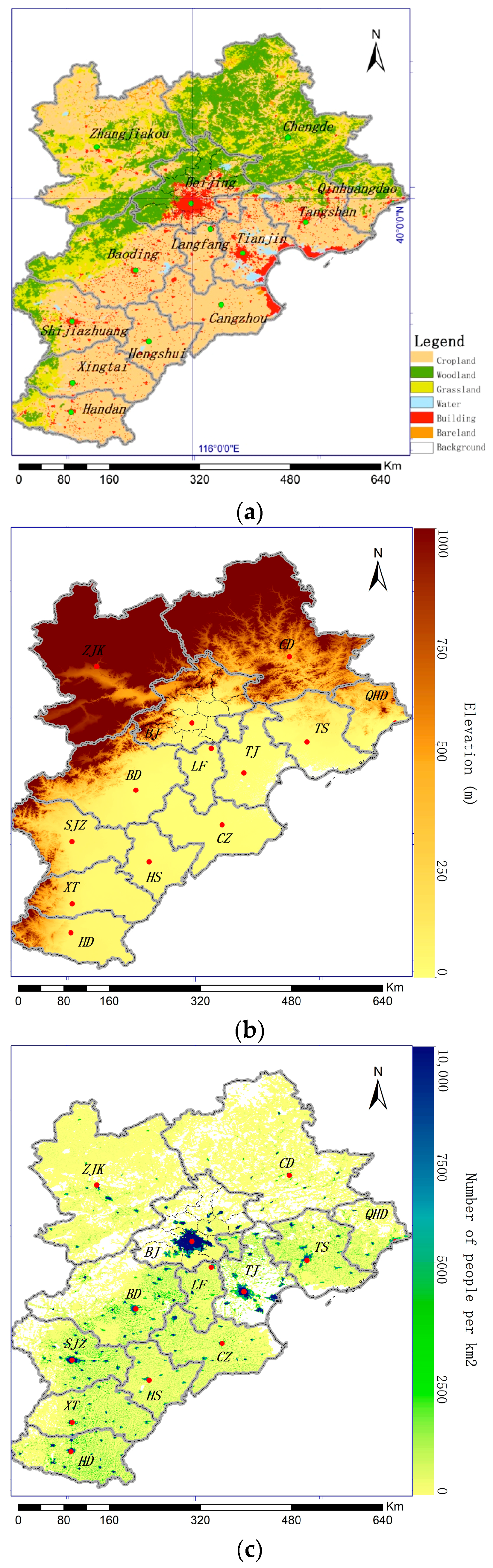
2.2. Research Region and City Samples

Beijing-Tianjin-Hebei is the largest metropolitan region in North China aside from the Bohai Bay area and is one of three regional economic centers (i.e., the Beijing-Tianjin-Hebei region, Yangtze River Delta and Pearl River Delta). Figure 1 displays the basic information regarding the land-use type, elevation, and population data of the region. In this study, the 1 km × 1 km Beijing-Tianjin-Hebei land-use data, population statistics for China and gross domestic product (GDP) statistics for 2010 were obtained from Global Change Research Data Publishing & Repository (http://geodoi.ac.cn/WebCn/DataSearch.aspx). The DEM data employed in this study were acquired by the NASA SRTM. Beijing-Tianjin-Hebei can be divided into two parts: the more populated southern and eastern sectors mainly comprise cropland located at lower elevations, while the northern and western sector is more mountainous and has a smaller overall population. In 2010, the population of Beijing-Tianjin-Hebei was 104.6 million, which accounted for 7.8% of the total population of China, and its GDP was CNY 1.95 trillion (USD 497.51 billion), which was approximately 10.99% of the gross GDP of China at that time. The area of Beijing-Tianjin-Hebei is 215,871 km2, which is approximately 2.25% of the total land area of China (statistics were obtained from the National Bureau of Statistics of China (http://data.stats.gov.cn/english/)). Both primary and secondary industries in Beijing-Tianjin-Hebei are highly developed. Due to industrialization, one of the most imperative challenges for the Beijing-Tianjin-Hebei region is air pollution [32]. Correspondingly, Beijing-Tianjin-Hebei exhibits severe air pollution, the pollutants of which include PM2.5, O3, NO2 and SO2, and the area also suffers from serious dust storms in the spring.
To investigate the study area in terms of different sampling regions, the averages of the pixels located within the various boundaries of an administrative shapefile were used to represent the various sample regions (i.e., prefectural-level-cities and corresponding urban areas). The spatial resolution of the OMI monthly gridded HCHO columns is 0.25° × 0.25°, which is capable of sufficiently covering urban areas. The ancillary data have a finer resolution than that of the TEMIS HCHO columns, and thus, an inverse distance weighted interpolation algorithm was adopted for re-sampling.

3. Results and Discussion

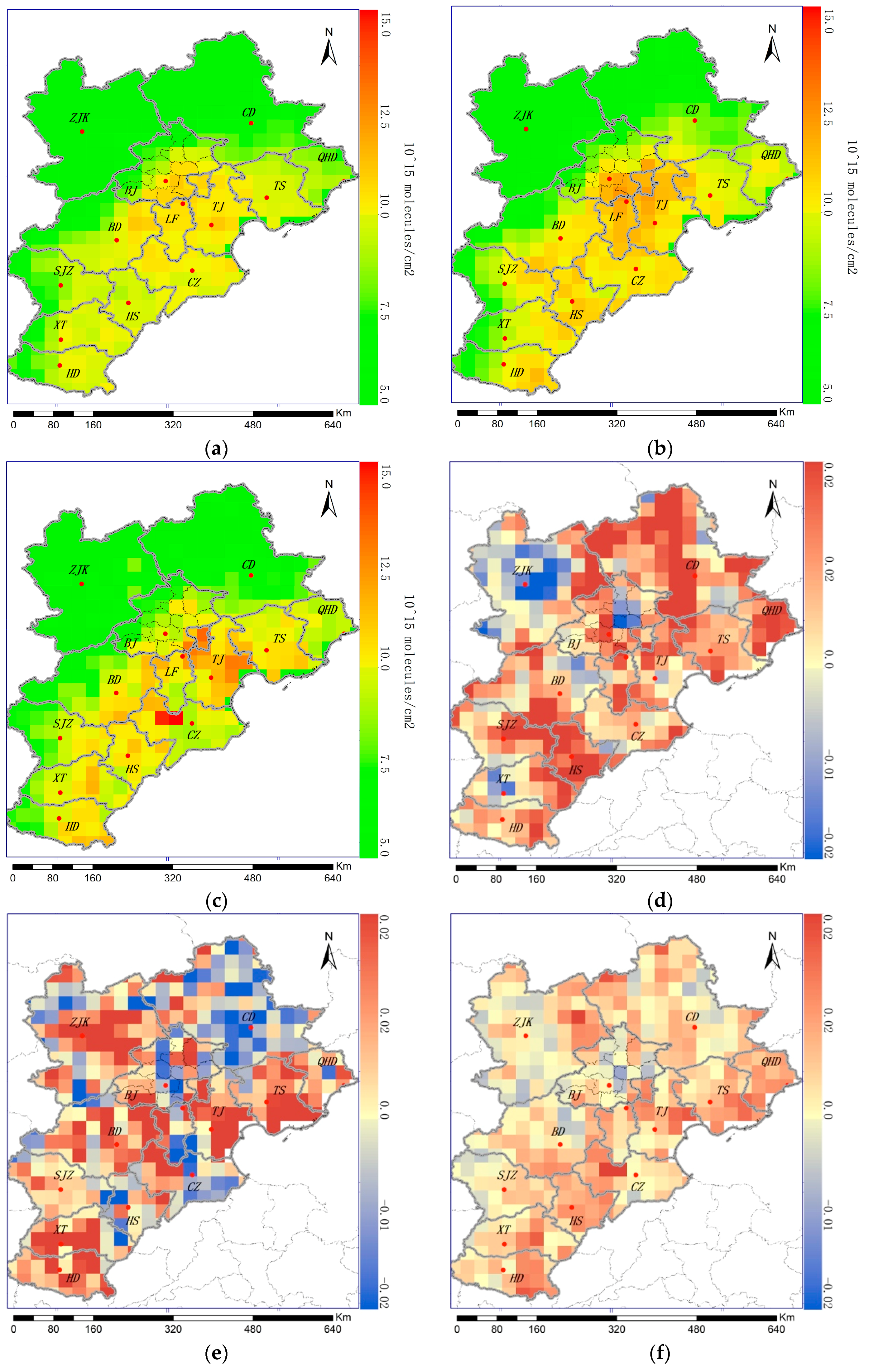
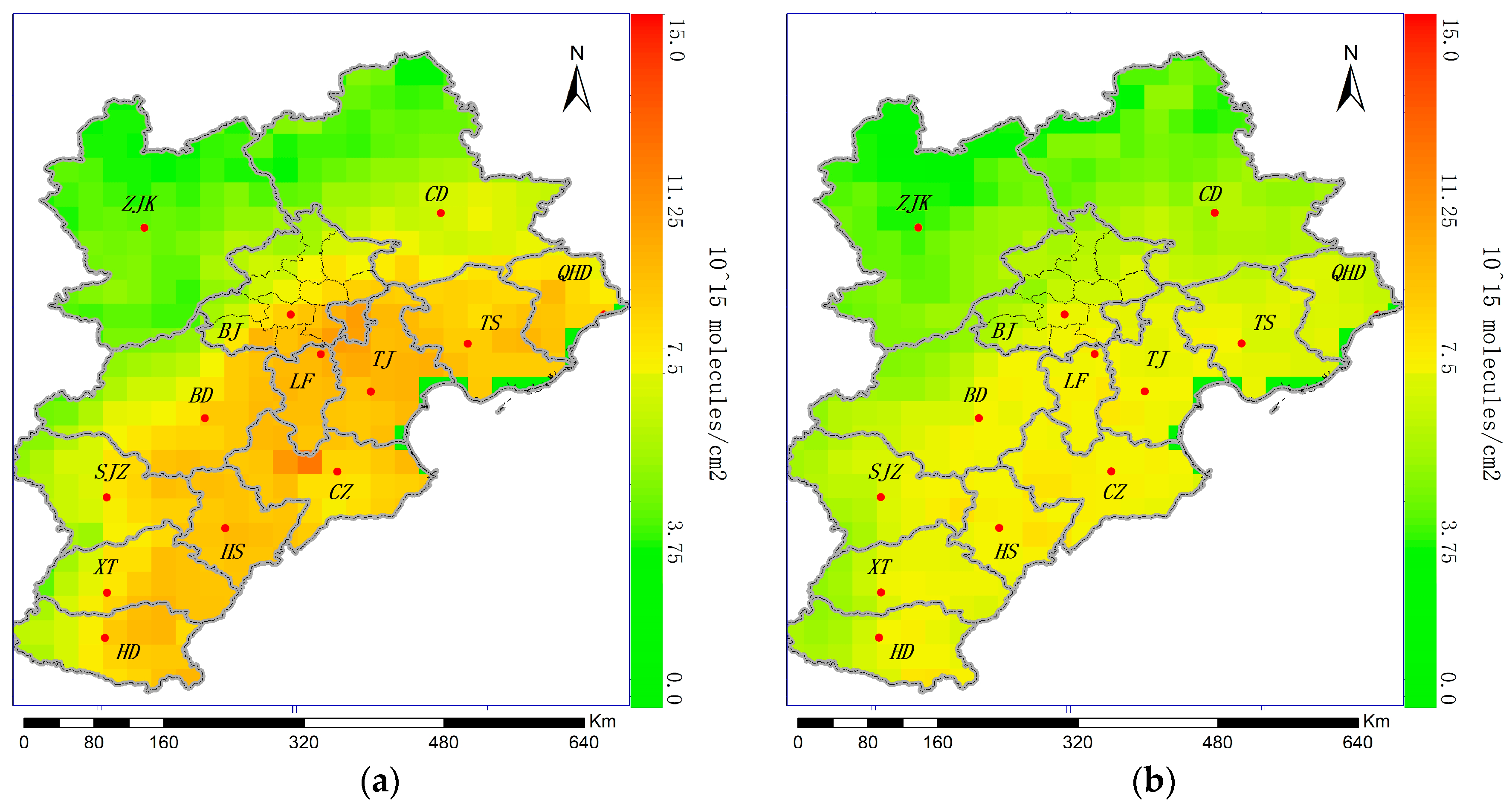
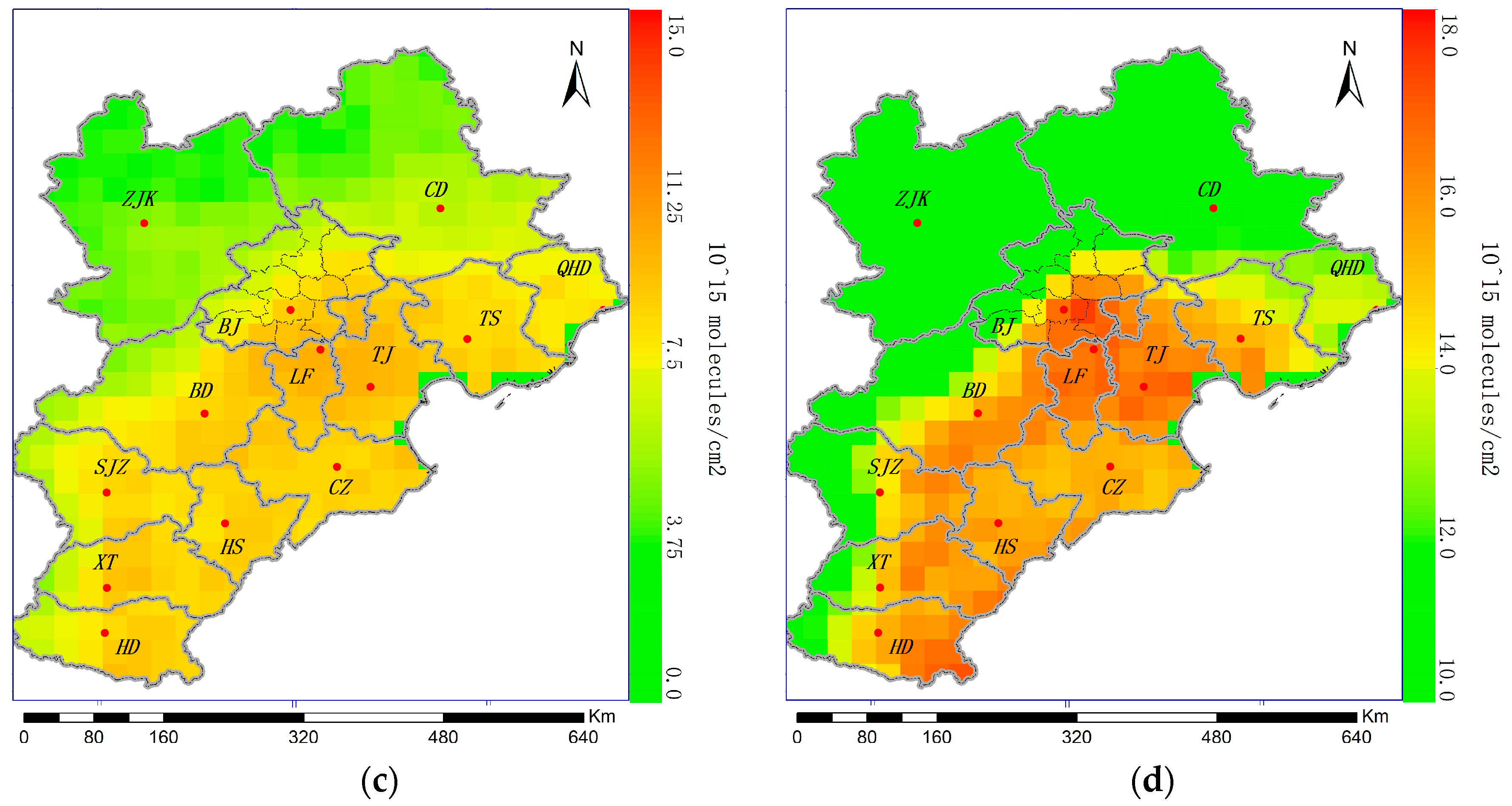
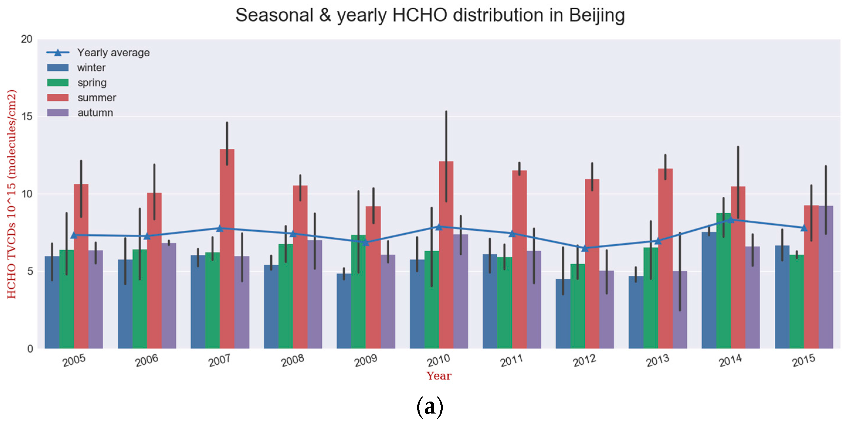
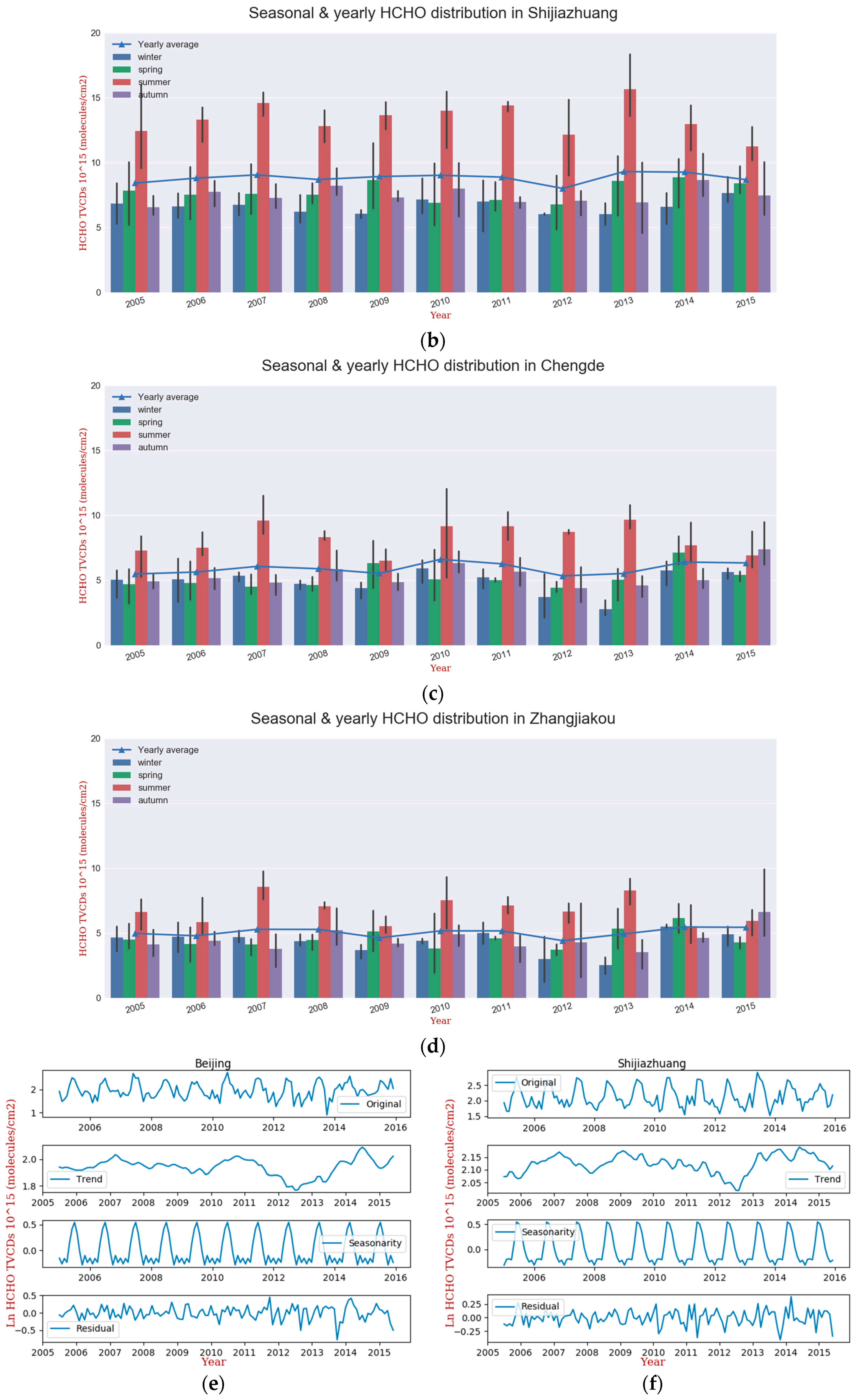
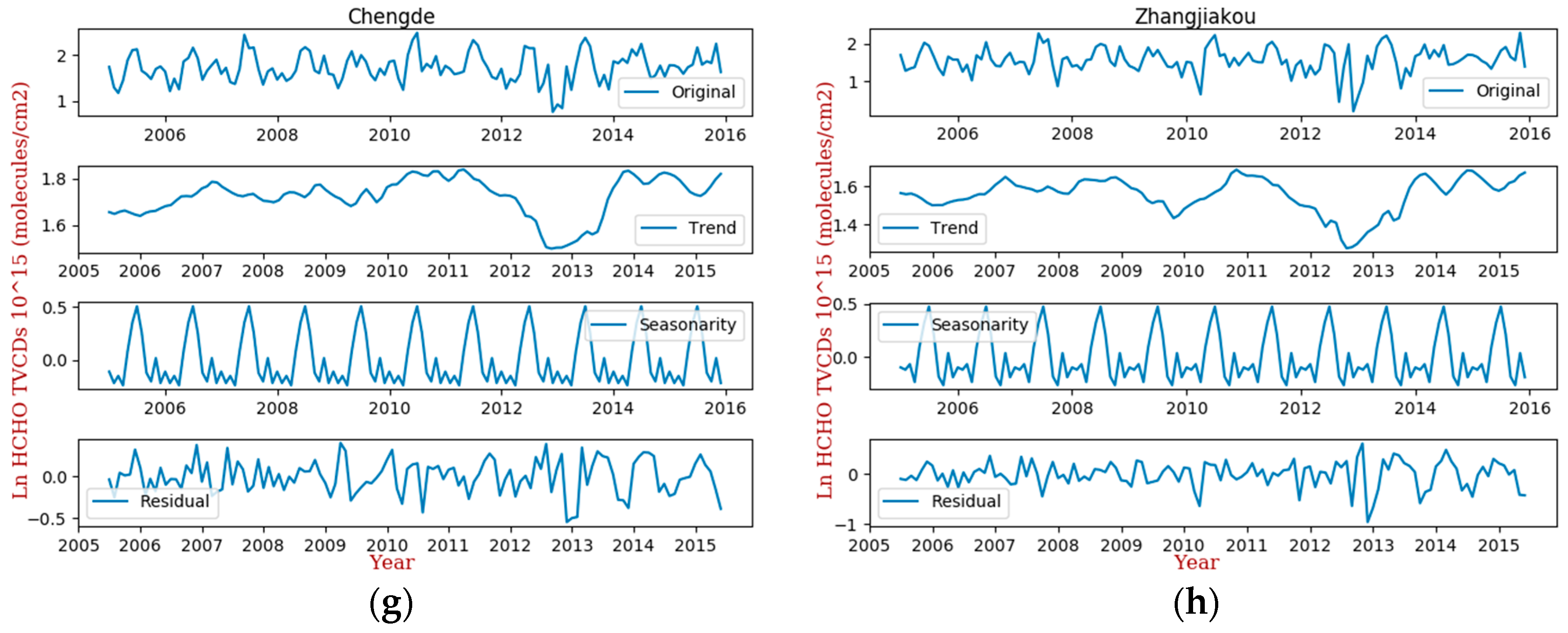
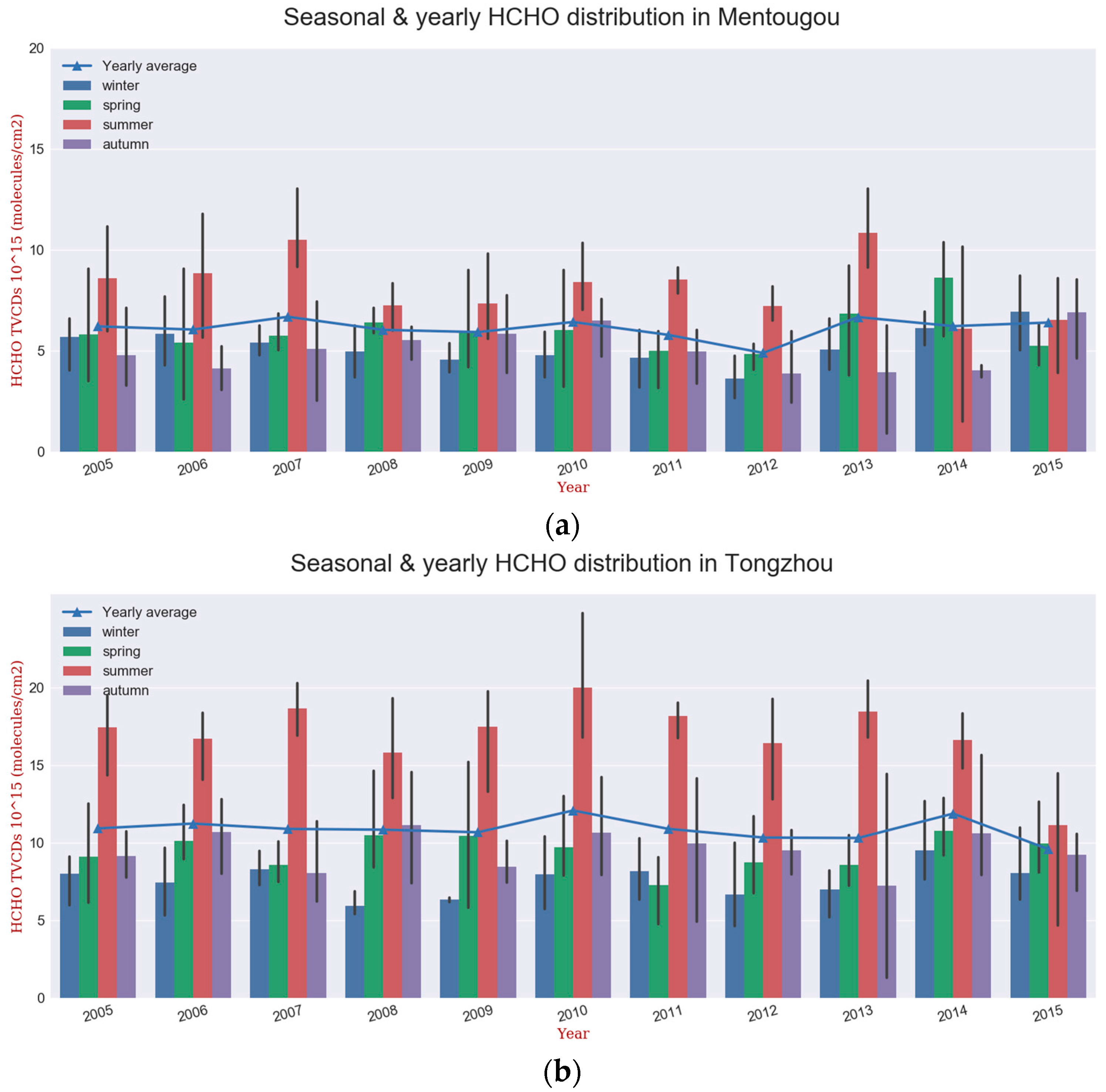
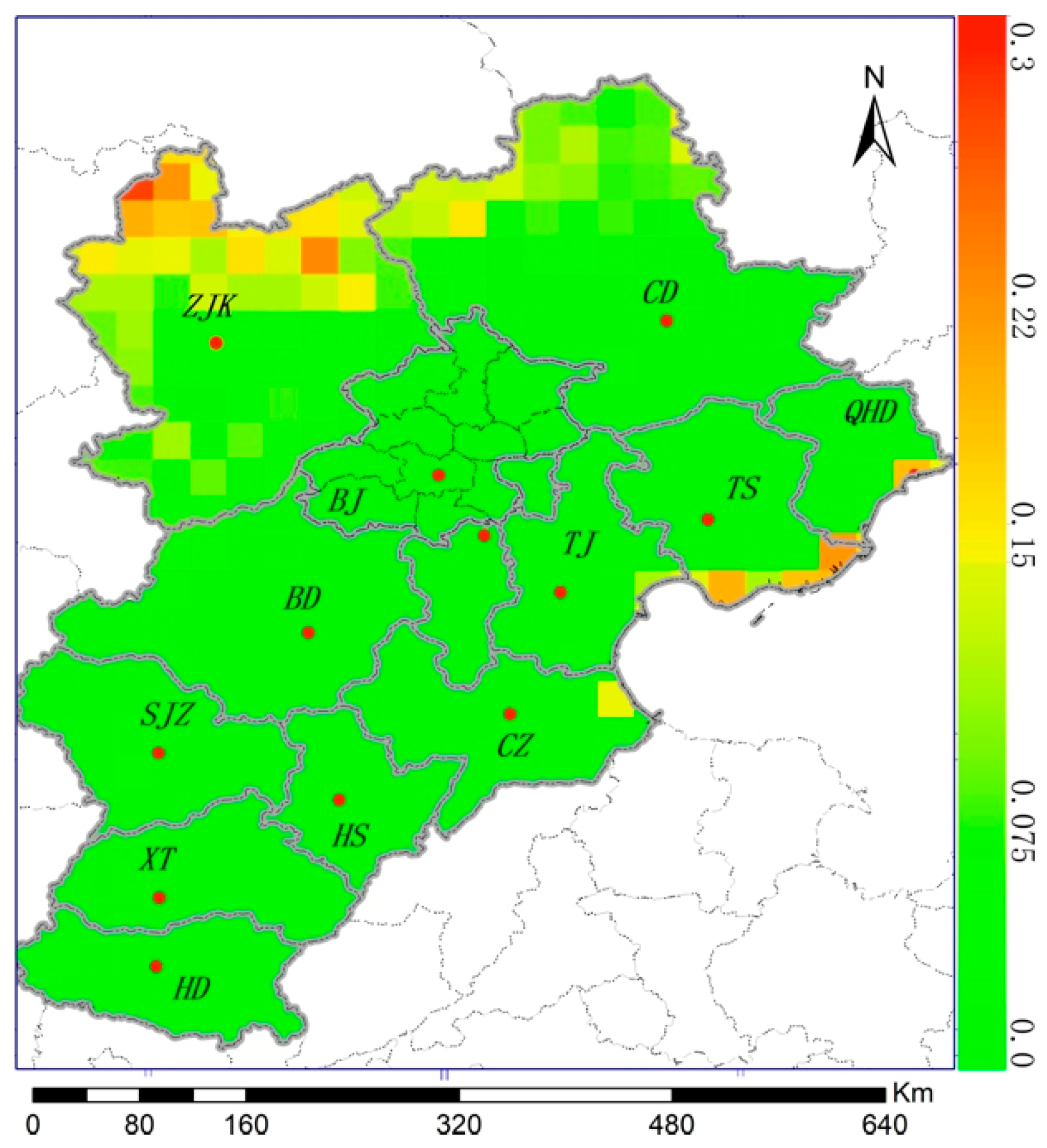
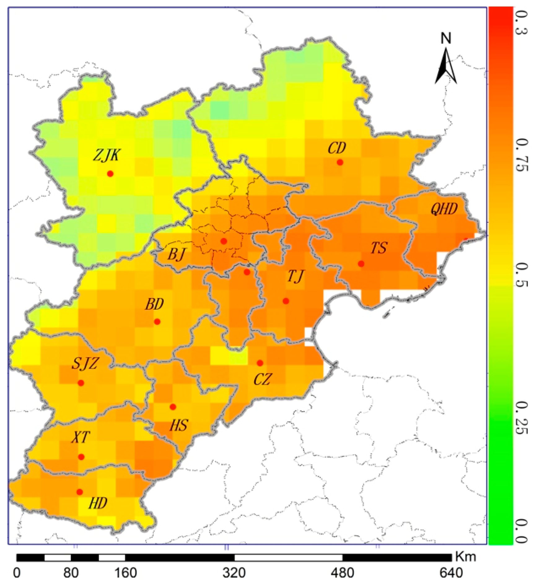
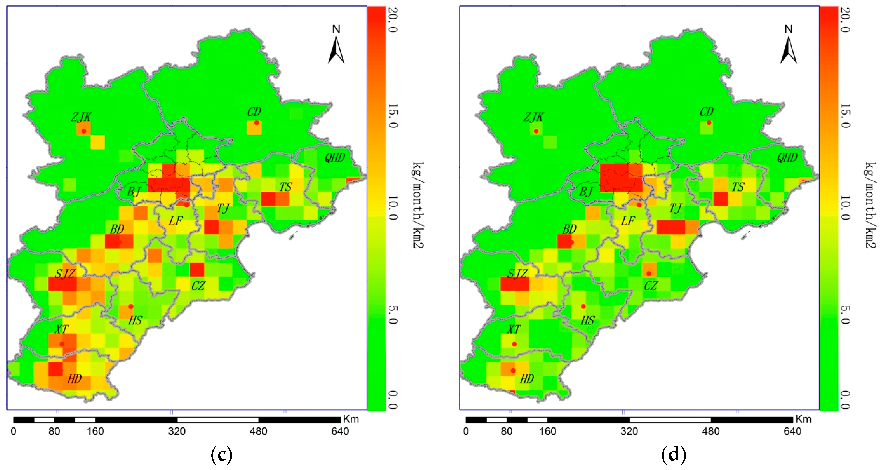
3.1. Spatiotemporal Distribution Features of HCHO throughout Beijing-Tianjin-Hebei

Although uncertainties have been largely reduced in HCHO products, it is possible that other systematic errors have not been eliminated entirely. Regarding the potential instrumental error, HCHO over the remote Pacific Ocean has been taken into consideration. As reported, HCHO over the western Pacific Ocean (i.e., the HCHO background area) was used to validate corresponding satellite-based measurements, and no trend was found [33,34]. Linear least squares regression adopted in this study is the approach to infer the potential trends exhibited in HCHO images. Given that, eleven-year average columns and corresponding trends over two remote Pacific areas (i.e., tropical Pacific (180°–160° W 0–20° N) and mid-latitude north Pacific (160°–180° E, 33°–43° N)) were used as the reference and potential impact of instrument uncertainty. The remote tropical Pacific (with an average VCD of 3.8 × 10¹⁵ molecules/cm2 and a deviation of 3 × 10¹⁴ molecules/cm2) is the broadly adopted background area, and the mid-latitude north Pacific (with an average VCD of 3.9 × 10¹⁵ molecules/cm2 and a deviation of 5 × 10¹⁴ molecules/cm2) used in this study is located in almost the same latitudinal zone compared with Beijing-Tianjin-Hebei. Over the mid-latitude north Pacific, the average trend of HCHO VCDs is 3.00 × 10¹² molecules/cm2·month−1 compared with 2.70 × 10¹¹ molecules/cm2·month−1 over the tropical Pacific area. Therefore, the average column (i.e., 3.9 × 10¹⁵ molecules/cm2) and trend (i.e., 3.00 × 10¹² molecules/cm2·month−1) over mid-latitude north Pacific Ocean were considered as impact potentially imposed by noise.
Figure 2a–c show the yearly average values of the tropospheric HCHO VCD in 2005, 2010 and 2015, respectively. The eleven-year average HCHO VCD of the whole Beijing-Tianjin-Hebei region is 7.6 × 10¹⁵ molecules/cm2 and the standard deviation is 2.5 × 10¹⁵ molecules/cm2. The HCHO distribution exhibits significant and evident discrepancies toward the east and west. For example, the average HCHO VCD is approximately 10 × 1015 molecules/cm2 toward the south and east, while the VCD is only approximately 5 × 10¹⁵ molecules/cm2 in the other sectors (Figure 2b). Higher HCHO VCDs are more easily observed over the densely populated plains (e.g., the southern and eastern sector) shown in Figure 1. In contrast, most of the regions with lower HCHO VCDs are mountainous with a smaller population. The widespread distribution of HCHO is more homogenous than those of other gaseous pollutants (e.g., NO2), and no HCHO concentration center is observed within the satellite images.
From 2005 to 2010 (Figure 2d), the HCHO concentration increased throughout most of Beijing-Tianjin-Hebei except for a selected few locations. The largest increase was observed in Chengde (i.e., the trend is 1.40 × 10¹³ molecules/cm2·month−1 with an RMSE about 2.6 × 10¹⁵ molecules/cm2). This might be due to the rapidity of urbanization and industrial development in China, including within the Beijing-Tianjin-Hebei region, which is accompanied by vast quantities of emissions that can cause serious air problems. Figure 2e shows the changes in HCHO VCDs through 2010 to 2015, which possibly reflect the strict reduction policies regarding VOCs that became public during that interval. Evident downward trends were found in Beijing, Cangzhou and Langfang at −7.39 × 10¹² molecules/cm2·month−1, −1.80 × 10¹³ molecules/cm2·month−1, and −7.83 × 10¹² molecules/cm2·month−1, respectively, especially in the heavily urbanized areas. HCHO columns in Chengde were largely reduced by about 17% during that period, although a VCD increase was observed therein between 2005 and 2010. In contrast, Zhangjiakou exhibited a distinct increase from 2010 to 2015, and about 35% in urban areas. This increase is likely due to the recent development of western Beijing-Tianjin-Hebei. In addition, although decreases were observed in northern sectors (e.g., Chengde) from 2010 to 2015, to gather a general picture in both periods, Beijing-Tianjin-Hebei, on average as suggested in Figure 2f, demonstrates an overall upward trend (5.20 × 10¹³ molecules/cm2·month−1 with a deviation of 3.6 × 10¹⁵ molecules/cm2) from 2005 to 2015. The findings are generally consistent with previous work, for instance, De Smedt et al. identified increasing HCHO columns in China [16]. Temporal and spatial discrepancies in HCHO distribution are complicated in mega-cities like Beijing [35]. Therefore, more specific analyses will be discussed later.
The seasonal features and patterns of the HCHO distribution are discernable for every year between 2005 and 2015. Figure 3 demonstrates the average seasonal tropospheric HCHO VCDs. Figure 3a shows the HCHO VCD distribution during the autumn season. The average VCD in autumn is 6.8 × 10¹⁵ molecules/cm2 and the standard deviation is 2.9 × 10¹⁵ molecules/cm2. High contiguous HCHO concentrations were observed primarily within the Beijing-Tianjin-Tangshan industrial area. Some high VCDs were also observed in the southern parts of the study area. Figure 3b depicts the HCHO VCD distribution during the wintertime with an average of 5.79 × 10¹⁵ molecules/cm2 and a deviation of 1.5 × 10¹⁵ molecules/cm2. Emissions during the winter season (e.g., in Beijing) are primarily derived from anthropogenic sources, as emissions from deciduous trees are enormously diminished [36]. Consequently, biogenic VOC photolysis is relatively inactive, and the distribution of HCHO is decreased substantially.
Figure 3c illustrates the HCHO distribution during the spring. Compared to that in the winter season, the coverage and VCD of the HCHO distribution in spring barely changes; however, a large zone of high HCHO concentrations appears in Beijing-Tianjin-Langfang. In spring, HCHO distribution is similar to that in autumn with an average of 6.7 × 10¹⁵ molecules/cm2 and a deviation of 2.1 × 10¹⁵ molecules/cm2. Figure 3d shows the HCHO distribution in summer, during which both the vegetation activity (e.g., isoprene) and sunlight intensity reach their peaks. The entire southern and eastern Beijing-Tianjin-Hebei region exhibits a very high HCHO concentration at 11.1 × 10¹⁵ molecules/cm2 with a standard deviation of 4.3 × 10¹⁵ molecules/cm2. The highest HCHO concentration was observed over southeast Beijing and surrounding areas (e.g., 16.6 × 10¹⁵ molecules/cm2 in Langfang). In addition, urban areas demonstrate relatively higher HCHO columns. For example, in southeast Beijing, a highly urbanized area, the average VCD is 12.9 × 10¹⁵ molecules/cm2 while the average VCD of the whole Beijing is 10.8 × 10¹⁵ molecules/cm2.
Furthermore, long-term datasets of HCHO VCDs for these regions were analyzed. As shown in Figure 4, the prefecture-level-cities of Zhangjiakou, Chengde, Beijing and Shijiazhuang are the most representative of the characteristics in western, northern, central and southern Beijing-Tianjin-Hebei, respectively. Each upper sub-plot of Figure 4 depicts the yearly and seasonal averages of the HCHO VCD throughout the whole administrative region. Most of the cases have the highest HCHO concentration during the summer, and the differences in the VCDs between the summer and the other seasons decreased rapidly following 2013 since when stricter policies enacted.
Additionally, the more industrialized cities show higher summertime columns, but a regional disparity was observed as well. The eleven-year averages over the whole prefecture-level-cities of Beijing and Shijiazhuang are 7.4 × 10¹⁵ molecules/cm2 and 8.8 × 10¹⁵ molecules/cm2, respectively. In contrast, the annual VCD averages in Chengde and Zhangjiakou are lower, i.e., approximately 5.9 × 10¹⁵ molecules/cm2 and 5.1 × 10¹⁵ molecules/cm2, respectively. The annually averaged VCD is relatively higher in urbanized areas, which are possibly characterized by more intense human activity. For example, the eleven-year averages in urban areas of Chengde and Zhangjiakou are 6.5 × 10¹⁵ molecules/cm2 and 5.0 × 10¹⁵ molecules/cm2, respectively.
The moving average technique and time series decomposition are beneficial for differentiating trends and extracting cyclical patterns [33,37,38]. The lower sub-plots demonstrate the results of time series decomposition (i.e., the trend component, seasonal component and the residual component). The p-values of the first-order-difference series are 3.90 × 10⁻¹⁵, 1.43 × 10⁻¹³, 9.68 × 10⁻¹⁹ and 6.85 × 10⁻¹² in Beijing, Shijiazhuang, Chengde and Zhangjiakou, respectively. The first-order-difference series was calculated based on the logarithms to original series, and the small p-values indicate that the results of decomposition are reliable. Except for the similar seasonal patterns, the trend components might reveal valuable details. As suggested, annual HCHO columns decreased since 2010 and significant upwards were found after 2012. Compared with corresponding summertime downward trends since 2013, the contributions from the other three seasons might have increased. Thus, inventories discussed in the next section are entirely possible to provide meaningful information.
Given this regional disparity, it is likely that some information might not be revealed from average values at the prefecture-level-city scale. Figure 5 shows the HCHO VCDs from 2005 to 2015 for two districts of Beijing. Beijing is well known as a megacity, and the levels of development among the different districts are unbalanced. Tongzhou District, an industrialized district in eastern Beijing, is more developed than Mengtougou District, which is a more rural district of western Beijing. Tongzhou clearly demonstrates a higher annually averaged HCHO VCD than Mengtougou (10.9 × 10¹⁵ molecules/cm2 and 6.1 × 10¹⁵ molecules/cm2, respectively), and the differences in the HCHO VCD during the summertime compared with those during the other seasons are larger in Tongzhou than in Mentougou. The HCHO VCDs over Tongzhou increased discontinuously from 2005 to 2010 at 1.30 × 10¹³ molecules/cm2·month−1, after which they decreased discontinuously from 2010 to 2015 at −4.41 × 10¹² molecules/cm2·month−1. In contrast, the HCHO VCDs in Mentougou did not change distinctly from 2005 to 2010 (i.e., the rate is 5.08 × 10¹¹ molecules/cm2·month−1 and it could all be noise) and increased from 2010 to 2015 at 6.00 × 10¹² molecules/cm2·month−1. This result is likely because of a greater degree of development in the western areas that lagged behind those of the eastern areas.
Errors in OMI HCHO columns are mainly caused by the row anomalies (i.e., errors caused by blockage effects, wavelength shifts, and stray light) and other instrumental degradation problems. From 2007 onwards, certain rows of OMI’s CCD detector were unavailable [39,40]. Due to the uncertainties in the sensor, inverse algorithm and in the gridding method, although systematic errors have been largely reduced, the impacts from these errors might still exist in results exhibited before. As reported in a previous study, meta data (i.e., XTrackQualityFlags) and a 0.15° × 0.15° Gaussian smooth filter of 1σ width were adopted and the median uncertainties of the HCHO gridded columns were reduced into 6% [40]. Additionally, spatial average and moving average methods were employed as discussed before to reduce systematic errors. Even so, it is undeniable that the potential instrumental errors might still impose an impact on the HCHO columns, and further deeper work will be conducted in the future.

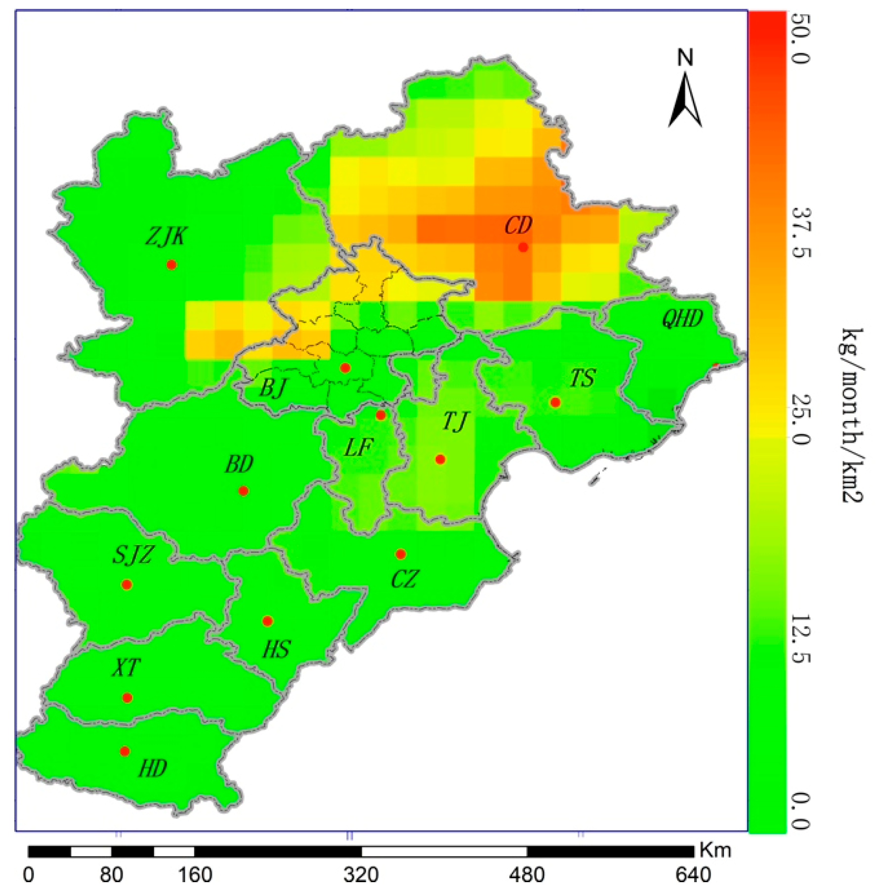
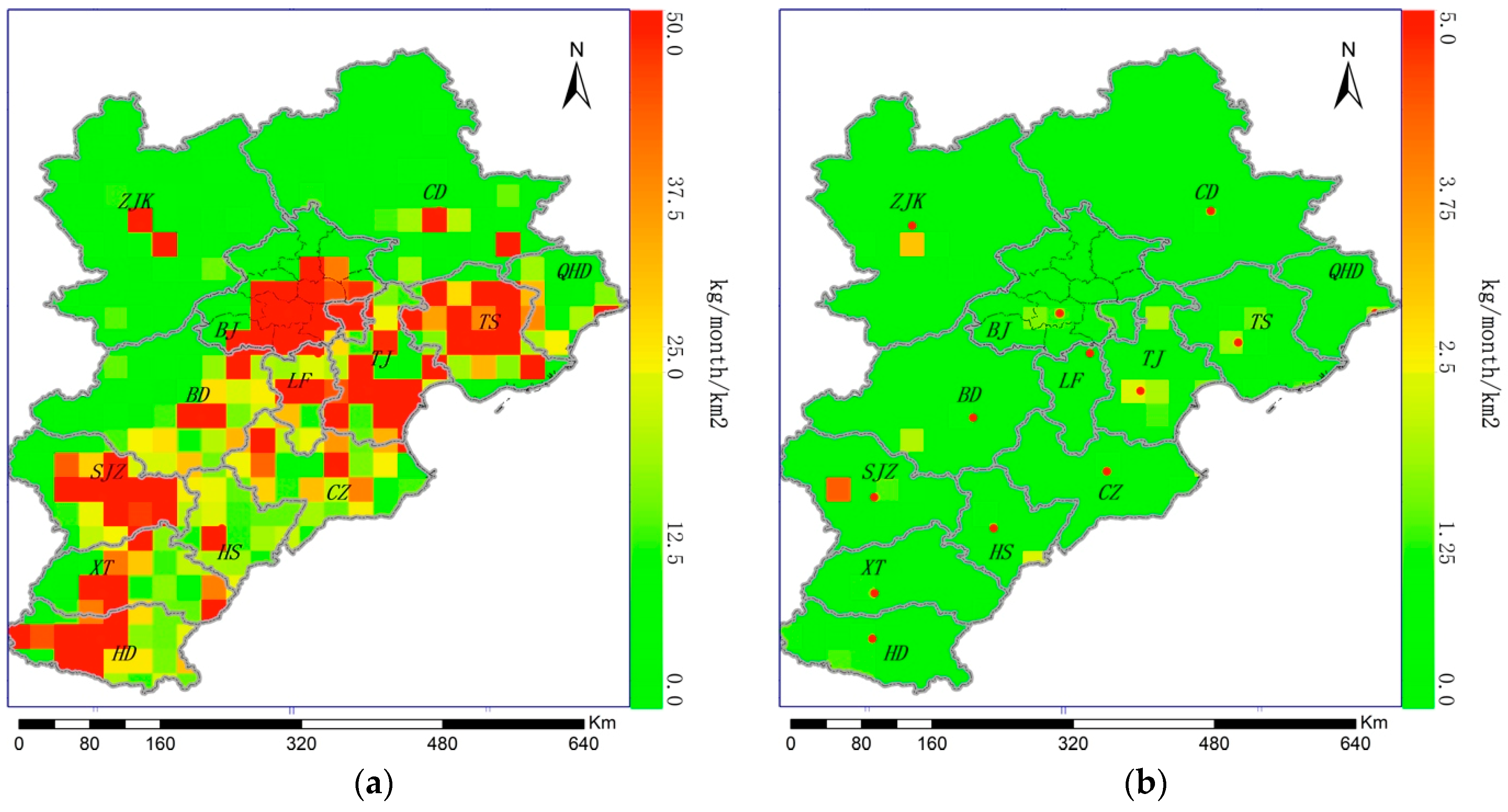
3.2. Analyses of Potential Factors for the HCHO Summertime Concentrations

In the continental boundary layer, HCHO as a high yield intermediate reaction product of the VOC oxidation and the smallest and most abundant aldehyde of oxygenated VOCs, is mainly generated from the oxidation of short-lived biogenic and anthropogenic NMVOCs [41]. In this section, we will discuss biogenic and anthropogenic sources of HCHO, and whether direct HCHO emissions constitute a substantial contribution to pollution will be determined. Figure 6 shows the Moran’s I values for the tropospheric HCHO columns in the summer of 2010. Moran’s I is a measure of the spatial autocorrelation of data employed for geographical information science purposes, and it is characterized by the correlation of a pixel with its surrounding pixels [42,43]. The values of Moran’s I, which indicates the spatial autocorrelation of singular variables, reveal that the HCHO distribution is less correlated. Table 1 provides the Moran’s I for urban areas of the whole Beijing-Tianjin-Hebei region. The average Moran’s I of Beijing-Tianjin-Hebei throughout eleven years is 0.04. In each year, the Moran’s I value of almost every urban area throughout Beijing-Tianjin-Hebei was less than 0.3 (e.g., the highest was 0.28 in 2014, Zhangjiakou), which essentially represents the lack of correlation and suggests the absence of cluster centers. The short lifetime and low Moran’s I values of HCHO strongly imply that high HCHO VCDs might not originate from direct primary sources of emission because short-lived gases from direct emissions (e.g., anthropogenic NO2) would concentrate around their emission sources. Therefore, these results suggest that the summertime HCHO VCDs might be generated from secondary sources (i.e., VOC photolysis).
Isoprene is found to be responsible for about 30% of the HCHO formed on the global scale [44]. As discussed in Section 3.1, the summertime concentration of HCHO demonstrated an obvious seasonal pattern that corresponded to periods of enhanced vegetation activity. This pattern repeated itself among all the years from 2005 to 2015. For example, the HCHO distribution in Beijing was observed to have a higher VCD in the summertime than during the winter, and photochemical reactions during the summer are the major source of HCHO emissions [18]. Isoprene emissions from deciduous trees in Beijing were also observed to be a substantial source of HCHO [45]. In addition, the areas with high HCHO VCDs to the south and east are croplands except for some smaller areas of residential buildings. Biogenic emissions are more active than those of anthropogenic VOCs, and the large quantities of emissions in the southern sector are highly influential and consequently affected the results of the long-term series [46,47]. Duncan et al. noted that BVOC emissions are exponentially correlated with the temperature and that BVOC emissions peak over the North China Plain in August [48,49]. Furthermore, Figure 7 shows the PCCs of both normalized HCHO VCDs and the NDVI for eleven years throughout Beijing-Tianjin-Hebei. The PPCs are higher in the southern and eastern sectors of Beijing-Tianjin-Hebei, which demonstrates higher HCHO VCDs. Table 2 and Table 3 provide the PCCs for three sample pixels in the southern and eastern areas and average PCCs for prefecture-level-cities and corresponding urban areas, respectively. The PCCs in southern and eastern sectors are higher than 0.6, especially in the northern parts (e.g., Beijing, Tianjin and Tangshan). In contrast, the PCCs are comparatively lower in northwestern Beijing-Tianjin-Hebei. Generally, PCCs in urban areas are higher than in the whole prefecture-level-cities. Combined with Figure 3d, it appears that the prefecture-level-cities with higher HCHO VCDs have higher PCCs, which might imply that vegetation could represent a substantial contributor.
Although the correlation between HCHO and vegetation (i.e., the NDVI) is relatively high, the factors of summertime HCHO concentrations are more complicated than expected. The PCCs are higher in urban areas, and relatively higher VCDs are mainly distributed throughout the southeastern sectors that are more industrialized and have a larger population. In addition, the spatial PCC between HCHO VCDs and NDVI in summertime is 0.012 with 2-tailed p-value as 0.87, and this suggests the spatial correlation between HCHO VCDs and vegetation activities is not as good as assumed. The p-value is widely used to quantify the statistical significance. If the p-value is smaller than 0.05 then it is significant and the correlation is obvious. It is noteworthy that to decrease the uncertainty, the calculation of spatial PCCs was conducted among the county-level averaged values rather than singular pixels. These observations might suggest anthropogenic sources as a substantial contributor.
Figure 8 shows the distribution of isoprene emissions in 2010 that was derived from the MEGAN model. The distribution patterns of isoprene (i.e., the precursor of secondary biogenic HCHO) were found to be opposite to the satellite-based HCHO distribution. Biogenic HCHO emissions in the northern areas of Beijing-Tianjin-Hebei (e.g., about 19.42 kg/month/km2 in Chengde) are higher than in the southern and eastern area (the average is 7.92 kg/month/km2), and the spatial PCC between HCHO VCDs and isoprene emissions is −0.21 with a 2-tailed p-value of 0.006. Additionally, isoprene is primarily generated from deciduous trees, which are common throughout northern Beijing-Tianjin-Hebei; however, the land-use types in southeastern sectors with high HCHO VODs are mainly cropland. Over China, isoprene fluxes were found to decrease from 8.6 Tg in 2007 to 6.5 Tg in 2012, and a significant emission decline was found after 2007 (−25% in 5 years) by using formaldehyde as a proxy for VOC emissions [44].
Although the seasonal HCHO patterns correspond with the periodic characteristics of vegetation activity, anthropogenic VOC emissions might be an influential contributor for the relatively high columns in southeastern Beijing-Tianjin-Hebei. Anthropogenic emissions are a major source of VOCs in China, and Beijing-Tianjin-Hebei is an important industrial zone in the north. Thus, the observed HCHO VCDs could have possibly originated from anthropogenic sources [6]. Meanwhile, HCHO is mainly concentrated within the more densely populated parts of Beijing-Tianjin-Hebei, in which emissions from industries and vehicles cannot be neglected. Consequently, it is entirely possible that the high levels of HCHO in the summertime are caused by anthropogenic sources. To shed light on that, an accurate inventory is essential for air-quality simulations and policy making, but available anthropogenic inventory data are insufficient [50]. Therefore, inventories provided by MEIC are important and valuable.
In this manuscript, yearly averaged MEIC inventories were used to evaluate anthropogenic emissions over Beijing-Tianjin-Hebei region. For each emission sector (i.e., industrial, power-based, residential and transportation), the monthly distribution range barely changed from 2008 to 2012 with 36-month averaged spatial PCCs of 0.97, 0.97, 0.94 and 0.96, respectively. The corresponding standard deviations of monthly spatial PCCs for four sectors are 0.02, 0.02, 0.03 and 0.03, respectively. In addition, all corresponding p-values of the spatial PCCs are smaller than 1 × 10−50, indicating the results are reliable. The three-year averaged change rates were used to represent temporal variations of four sectors. The change rates are 0.64, 0.03, −0.49 and −0.03 kg/month/km2 per month for industrial, power-based, residential and transportation sectors. The corresponding standard deviations are 0.33, 5.9 × 10⁻⁴, 0.20, 0.03 kg/month/km2 per month, respectively. The monthly change of each anthropogenic source is relatively small in each year and the yearly averaged emissions adopted in this study are relatively plausible.
Anthropogenic VOC emissions contribute more than 40% to the total reactive NMVOC emissions (i.e., VOCs would produce HCHO) in China, while biogenic activities and biomass burning contribute about 50% and 6%, respectively [6]. Figure 9 shows the MEIC anthropogenic VOC inventories for Beijing-Tianjin-Hebei during the summer of 2010. Compared with those of BVOCs, anthropogenic VOC emissions change little from June to August [35]. According to the MEIC, agricultural sources did not constitute any VOC emissions in Beijing-Tianjin-Hebei.
Figure 9a displays the industrial VOC emission rates. Compared with isoprene emissions of 9.44 kg/month/km2 with a standard deviation of 8.03 kg/month/km2, the industrial VOC emission rates are much higher at 22.25 kg/month/km2 but with a lager deviation at 54.22 kg/month/km2 as well. Table 4 provides the spatial PCCs between HCHO VCDs and anthropogenic VOC emissions and corresponding p-values. Evidently, the distribution of industrial VOC emissions corresponds with that of HCHO columns more than isoprene with an average spatial PCC about 0.30. Figure 9b shows the power-based VOC emission rates. Compared with the industrial sources, power-based emissions maintain lower rates of approximately 0.09 kg/month/km2 with a standard deviation of 0.35 kg/month/km2 and are discretely distributed throughout suburban areas. Additionally, spatial PCCs between power-based VOC emissions and HCHO VCDs are also comparatively low, and a downward trend has been observed.
The residential sources as depicted in Figure 9c have a very similar distribution as the industrial sources but with much lower emission rates. The average residential emission rate is 4.61 kg/month/km2 with a standard deviation of 6.78 kg/month/km2, and the emissions are mostly concentrated in urban areas. However, the spatial PCC between HCHO VCDs and residential sources is the largest, indicating that residential sources are a potentially important contributor even though their emission rate is quite smaller than industrial and biogenic ones. As shown in Figure 9d, the transportation sources are sparsely located among the urban areas. The average is 3.79 kg/month/km2 and the standard deviation is 9.61 kg/month/km2. The spatial PCC of transportation is the second largest and no continuous trend was observed. This is possibly related to annual registered vehicle amounts and the control policies on gasoline quality.
Table 5 gives average anthropogenic emission rates in each prefecture-level city throughout the Beijing-Tianjin-Hebei region. Among all regions, the industrial sources are the most substantial, i.e., more than 70% in almost all cities (e.g., 75.16% in Beijing, 71.84% in Shijiazhuang, 73.60% in Chengde and 72.88% in Zhangjiakou). Southeastern sectors demonstrate higher industrial emissions than other sectors. For example, emissions in Langfang were approximately an order of magnitude higher than in Chengde in 2012. In addition, industrial emissions increased largely from 2008 to 2012, suggesting a close connection to the rapid industry development. Tangshan exhibits the largest increment at 49.15% and Shijiazhuang exhibits the smallest at 28.57%. In each year, on average, power-based sources contribute a very small fraction of VOC emissions in all cities (e.g., 0.17% in Beijing and 1.78% in Zhangjiakou).
Residential and transportation sources contribute in the same order of magnitude. Residential emissions demonstrate upward trends from 2008 to 2012 in almost every city. The largest and smallest were observed in Zhangjiakou and Tianjin with 14.34% and 5.27%, respectively. The increasing amplitude is smaller than that of industrial sources. In contrast to residential sources, transportation emissions decreased from 2008 to 2012. Beijing, Zhangjiakou and Langfang decreased the largest at 49.73%, 49.10% and 44.76%, respectively. The residential and transportation emissions constitute approximately 10% of the total, and larger cities have relatively higher transportation emissions. For example, in 2010, Beijing had a higher transportation contribution than the residential one with 15.23 to 9.44%. One the contrary, in Chengde, the ratio was 8.70 to 17.08%. The sizes and values of the residential and transportation sources are possibly dependent on many factors (e.g., the city size and the vehicle number).
Table 6 provides the anthropogenic VOC statistics corresponding to Table 5 but in urban areas. Compared with the averages in prefecture-level-cities, averages in urban areas are more related to human activities. Obviously, average industrial emissions in industrialized urban areas (e.g., Beijing and Tianjin) are much higher than in the whole prefecture-level-cities. Specifically, considering the three-year average, the average urban emission is about 3.37 times higher than that in the whole Beijing and in Tianjin the ratio is 7.23. On the contrary, less industrialized urban emissions (e.g., Chengde) are lower than those of the whole prefecture-level-cities because the locations of factories are influential. Trends are more complicated in urban areas, for example, in Beijing and Cangzhou, industrial emissions increased about 139.36% and 270.58% from 2008 to 2012, respectively. However, decreases were observed in Langfang and Qinhuangdao, i.e., −11.27% and −5.79%. The changes of industrial emissions in urban areas might be more dependent on local factors (e.g., implementation of reduction policies). It is likely that industrial VOC emissions worsen in cities like Beijing, especially in urban areas, and contribute more to HCHO pollution. Power-based VOC emissions account for a relatively small fraction, but it is noteworthy that they increased about 124.48% and 420.89% in urban Beijing and Shijiazhuang, and this might be influential in the future.
Residential and transportation emissions in urban areas are also higher than the prefecture-level-cities. For example, the ratio of urban emissions to prefecture-level-city ones is 2.22 for residential and 3.72 for transportation in Beijing. In addition, comparatively large cities have ratios larger than 1 (e.g., ratios in Tianjin and Shijiazhuang are all larger than 3.0). In relatively small cities, the ratio varies, and this might depend on many specific local factors. For residential sources, the emissions in urban areas increased in almost all cities with higher rates than emissions in prefecture-level-cities (e.g., 29.43% and 9.79% in Cangzhou, respectively). Meanwhile, transportation emissions decreased in almost all urban areas. Compared with residential sources, the difference of decreasing rates between urban areas and prefecture-level-cities varies more, suggesting that local factors might be important (e.g., city size, population and transportation conditions).
Isoprene is a well-known HCHO precursor, and its photochemical reactions are the predominant reason accounting for HCHO-induced air issues and subsequent surface O3 formation. Globally speaking, high-level HCHO columns in equatorial areas (e.g., tropical forests) have been observed via satellite-based platforms. The widespread summertime HCHO in Beijing-Tianjin-Hebei (i.e., locating in relative high latitudes) is unexpected. In this region, HCHO is mainly distributed in southeastern sectors, and the land-use types are not deciduous trees, which would emit isoprene, but cropland. Therefore, the sources of HCHO might be more complicated than expected. In this region, isoprene is mainly distributed in northern sectors (e.g., Chengde), and its distribution is opposite to that of HCHO. However, isoprene is still one major reason accounting for high-level HCHO columns because it is more active than anthropogenic VOCs. Further, anthropogenic VOCs might impose substantial impacts as well [20]. As reported, a continuous growth trend of China’s historical NMVOCs emissions was found during the period of 1980–2005, with the emission increasing by 4.2 times at an annual average rate of 10.6%; populous cities, covering merely 4.5% of China’s territory, accounted for 24.9% of the national emissions [51]. Additionally, results from the widely adopted MEIC inventories also suggest a similar consequence.
In this manuscript, potential contributions have been discussed as thoroughly as possible. The opposite distributions of HCHO columns and isoprene suggest that isoprene might not be the only reason accounting for high-level HCHO. The anthropogenic contribution was inferred from the relatively strong connection between HCHO columns and human activities in urbanized areas. In addition, the spatial PCCs of HCHO VCDs with anthropogenic VOCs are much higher than those of HCHO with isoprene, that is, the HCHO’s distribution is more similar to anthropogenic VOC distribution. In addition, active anthropogenic NMVOCs were observed with a larger amount than isoprene. Accordingly, anthropogenic sources cannot be neglected and might be substantially influential in the summertime HCHO concentration over southeastern Beijing-Tianjin-Hebei.
Nevertheless, the specific contributions in terms of VOC species (e.g., alkanes, aromatics, alkenes and alkynes, carbonyls) are still complicated. Currently, available inventories only provide VOC amounts for public use, and more detailed data are very limited [50]. Accordingly, quantitative determination of exact species-based VOC contribution is very difficult. At present, based on the MEIC inventories, industrial VOCs account for a relatively large amount of the total, and the residential sources exhibit the most similar distribution to that of HCHO columns. Therefore, anthropogenic emissions regarding industrial and residential sources might need to be taken into consideration with more concern. These results correspond with previous studies that suggest industry was the single largest anthropogenic sources and residential was the second largest in North China Plain [6]. In addition, Souri et al. suggested predominant anthropogenic VOC emissions account for high HCHO levels in urban regions, and mostly increasing HCHO columns were found [20].
In addition to biogenic and anthropogenic sources, pyrogenic sources also contribute to VOC emissions. As suggested, agricultural residue burning might impose influential impacts on HCHO contribution in June [52]. Bauwens et al., used a long record of OMI HCHO observations to infer emissions from pyrogenic and biogenic sources on the global scale, suggesting that isoprene fluxes in China are reduced and the pyrogenic emissions are regionally low [53]. Additionally, as discussed before, the contribution from pyrogenic sources accounts for 6% of the total active VOCs. Therefore, due to the lack of accurate pyrogenic data and the large discrepancies in different biomass emissions inventories, the detailed analysis regarding biomass burning is beyond the scope of this study. However, in the future, long-term pyrogenic VOC emission records (e.g., inventories like GFAS and FINN v 1.5) will also be incorporated to conduct a more comprehensive analysis.

4. Conclusions

In this manuscript, we studied 11 years of monthly globally gridded tropospheric HCHO columns from Beijing-Tianjin-Hebei and analyzed both annual and seasonal patterns. In addition, the biogenic and anthropogenic sources of VOCs, which are closely related to high summertime HCHO concentrations, were investigated. Based on data from the Aura OMI, a widespread distribution of high-latitude tropospheric HCHO VCDs was observed over the southern and eastern sectors of Beijing-Tianjin-Hebei. This large-scale coverage of high HCHO VCDs extending over the whole North China Plain and Yangtze River Delta is unique to the Northern Hemisphere. Beijing-Tianjin-Hebei was selected as the region of interest because of its socioeconomic importance, severe air pollution issues and the distinct difference between northwestern and southeastern sectors.
An overall increasing trend of HCHO columns from 2005 to 2015 was observed in this region. Specifically, due to rapid regional development, the HCHO columns increased from 2005 to 2010 over many areas of Beijing-Tianjin-Hebei and declined in the north (e.g., Chengde) from 2010 to 2015. This slight decline was potentially the result of strict regulations. In all sampling cities, according to the time series decomposition technique, HCHO VCDs declined steeply in 2013 and then increased rapidly. In terms of seasonality, HCHO in summertime demonstrated the largest concentration throughout the whole southeastern sectors. In addition, HCHO, assisted by calculating zonal statistics, in urban areas was observed with higher columns in stark contrast to the HCHO concentrations in rural areas.
Regarding the sources of HCHO, the low Moran’s I values and the short lifetime suggest that HCHO in Beijing-Tianjin-Hebei might not originate from primary sources but from secondary formation. Despite the universally good PCCs between HCHO and the NDVI, vegetation emissions might not be the only major factor accounting for the high concentration in southeastern sectors. The land-use types are cropland in these sectors and the spatial PCCs of NDVI and isoprene were relatively low, suggesting that the distribution of biogenic sources was not similar to that of HCHO. Given the relatively large amount of anthropogenic VOC emissions, the anthropogenic sources potentially impose important influence as well. In addition, compared with isoprene, the spatial distributions of anthropogenic VOCs and HCHO were more similar. Among all, industrial emissions accounted for more than 70% of the anthropogenic VOCs, and residential emission exhibited the largest spatial PCCs. By comparison, power-based emissions only accounted for a small fraction of about 1%, and transportation sources exhibited a downward trend while HCHO columns increased. Therefore, industrial and residential sources should be taken in consideration in VOC control, and contributions from other sources should not be neglected. Additionally, the leading contributor in each city was also dependent on the local conditions.
The distribution of VOCs was capable of only roughly explaining the distribution and concentrations of HCHO because the HCHO VCDs also relied upon many other factors. In the future, the influence of oxidants (e.g., the distribution and concentration of NOx) should be introduced to conduct more in-depth investigations. Moreover, the relationships among the HCHO concentration, specific VOC species and meteorological conditions in this area must be examined in order to more quantifiably describe the regional HCHO characteristics throughout Beijing-Tianjin-Hebei.

Acknowledgments

This work was supported by the State Key Laboratories of Remote Sensing Science and Digital Earth Science, the National Natural Science Foundation of China (Grant No. 41571345 and 41501476), the Special Foundation for Free Exploration of State Laboratory of Remote Sensing Science (Grant No. Y1Y00202KZ), and the Major Projects of High Resolution Earth Observation System (Grant No. 32-Y20A18-9001-15-17-1), the National Key R&D Program of China (Grant No. 2016YFC0201507), and it was partially supported by the China Postdoctoral Science Foundation (Grant No. 2015 M580084, 2016T90083). The authors are grateful to Jianbin Gu and Han Zhang. We thank Qiang Zhang of Tsinghua University for providing the MEIC emission model and A. B. Guenther from the National Center for Atmospheric Research (NCAR) for the MEGAN biogenic emission model results. We also thank Yong Ge et al. for the experimental dataset used to investigate land-use pixels in subpixel maps for the Beijing-Tianjin-Hebei region (DOI:10.3974/geodb.2016.02.17.V1). We are sincerely thankful for the open-access nature of the monthly tropospheric HCHO and NO2 column data from TEMIS (http://h2co.aeronomie.be), and the other organizations that provided necessary data.

Author Contributions

Songyan Zhu, Xiaoying Li and Chao Yu conceived and designed the experiments; Hongmei Wang and Yapeng Wang analyzed the data and performed the experiments; Jing Miao and Songyan Zhu collected the data and wrote the paper.

Conflicts of Interest

The authors declare no conflict of interest.

References

  1. Wang, Y.; Zhang, Y.; Hao, J.; Luo, M. Seasonal and spatial variability of surface ozone over China: Contributions from background and domestic pollution. Atmos. Chem. Phys. Discuss. 2010, 10, 3511–3525. [Google Scholar] [CrossRef]
  2. Duncan, B.N.; Yoshida, Y.; Olson, J.R.; Sillman, S.; Martin, R.V.; Lamsal, L.; Hu, Y.; Pickering, K.E.; Retscher, C.; Allen, D.J.; et al. Application of OMI observations to a space-based indicator of NOx, and VOC controls on surface ozone formation. Atmos. Environ. 2010, 44, 2213–2223. [Google Scholar] [CrossRef]
  3. Sillman, S. The use of NOy, H2O2, and HNO3 as indicators for ozone-NOx-hydrocarbon sensitivity in urban locations. J. Geophys. Res. 1995, 100, 14175–14188. [Google Scholar] [CrossRef]
  4. Fu, T.M.; Jacob, D.J.; Palmer, P.I.; Chance, K.; Wang, Y.X.; Barletta, B.; Blake, D.R.; Stanton, J.C.; Pilling, M.J. Space-based formaldehyde measurements as constraints on volatile organic compound emissions in east and south Asia and implications for ozone. J. Geophys. Res. Atmos. 2007, 112, 382–388. [Google Scholar] [CrossRef]
  5. Choi, Y.; Kim, H.; Tong, D.; Lee, P. Summertime weekly cycles of observed and modeled NOx and O3 concentrations as a function of satellite-derived ozone production sensitivity and land use types over the Continental United States. Atmos. Chem. Phys. Discuss. 2012, 12, 6291–6307. [Google Scholar] [CrossRef]
  6. Jin, X.; Holloway, T. Spatial and temporal variability of ozone sensitivity over China observed from the Ozone Monitoring Instrument. J. Geophys. Res. Atmos. 2015, 120, 7229–7246. [Google Scholar] [CrossRef]
  7. González Abad, G.; Liu, X.; Chance, K.; Wang, H.; Kurosu, T.P.; Suleiman, R. Updated Smithsonian Astrophysical Observatory Ozone Monitoring Instrument (SAO OMI) formaldehyde retrieval. Atmos. Meas. Tech. 2015, 8, 19–32. [Google Scholar] [CrossRef]
  8. Guenther, A.B.; Jiang, X.; Heald, C.L.; Sakulyanontvittaya, T.; Duhl, T.; Emmons, L.K.; Wang, X. The Model of Emissions of Gases and Aerosols from Nature version 2.1 (MEGAN2.1): An extended and updated framework for modeling biogenic emissions. Geosci. Model Dev. Discuss. 2012, 5, 1–58. [Google Scholar] [CrossRef]
  9. Gao, W.; Tang, G.; Xin, J.; Wang, L.; Wang, Y. Spatial-Temporal Variations of Ozone during Severe Photochemical Pollution over the Beijing-Tianjin-Hebei Region. Res. Environ. Sci. 2016, 29, 654–663. [Google Scholar]
  10. Hao, J.; He, D.; Wu, Y.; Fu, L.; He, K. A study of the emission and concentration distribution of vehicular pollutants in the urban area of Beijing. Atmos. Environ. 2000, 34, 453–465. [Google Scholar] [CrossRef]
  11. Kaiser, J.; Wolfe, G.M.; Bohn, B.; Broch, S.; Fuchs, H.; Ganzeveld, L.N.; Gomm, S.; Häseler, R.; Hofzumahaus, A.; Holland, F.; et al. Evidence for an unidentified non-photochemical ground-level source of formaldehyde in the Po Valley with potential implications for ozone production. Atmos. Chem. Phys. 2014, 15, 1289–1298. [Google Scholar] [CrossRef]
  12. Luecken, D.J.; Hutzell, W.T.; Strum, M.L.; Pouliot, G.A. Regional sources of atmospheric formaldehyde and acetaldehyde, and implications for atmospheric modeling. Atmos. Environ. 2012, 47, 477–490. [Google Scholar] [CrossRef]
  13. Zhu, L.; Jacob, D.J.; Kim, P.S.; Fisher, J.A.; Yu, K.; Travis, K.R.; Mickley, L.J.; Yantosca, R.M.; Sulprizio, M.P.; De Smedt, I.; et al. Observing atmospheric formaldehyde (HCHO) from space: Validation and intercomparison of six retrievals from four satellites (OMI, GOME2A, GOME2B, OMPS) with SEAC4RS aircraft observations over the Southeast US. Atmos. Chem. Phys. 2016, 16, 1–24. [Google Scholar] [CrossRef]
  14. Barkley, M.P.; De Smedt, I.; Van Roozendael, M.; Kurosu, T.P.; Chance, K.; Arneth, A.; Hagberg, D.; Guenther, A.; Paulot, F.; Marais, E.; et al. Top-down isoprene emissions over tropical South America inferred from SCIAMACHY and OMI formaldehyde columns. J. Geophys. Res. Atmos. 2013, 118, 6849–6868. [Google Scholar] [CrossRef]
  15. De Smedt, I.; Müller, J.F.; Stavrakou, T.; Van Der A, R.; Eskes, H.; Van Roozendael, M. Twelve years of global observation of formaldehyde in the troposphere using GOME and SCIAMACHY sensors. Atmos. Chem. Phys. 2008, 8, 4947–4963. [Google Scholar] [CrossRef]
  16. De Smedt, I.; Stavrakou, T.; Hendrick, F.; Danckaert, T.; Vlemmix, T.; Pinardi, G.; Theys, N.; Lerot, C.; Gielen, C.; Vigouroux, C.; et al. Diurnal, seasonal and long-term variations of global formaldehyde columns inferred from combined OMI and GOME-2 observations. Atmos. Chem. Phys. 2015, 15, 12241–12300. [Google Scholar] [CrossRef]
  17. De Smedt, I.; Stavrakou, T.; Müller, J.F.; Van Der A, R.; Roozendael, M.V. Trend detection in satellite observations of formaldehyde tropospheric columns. Geophys. Res. Lett. 2010, 37, L18808. [Google Scholar] [CrossRef]
  18. Pang, X.; Mu, Y. Seasonal and diurnal variations of carbonyl compounds in Beijing ambient air. Atmos. Environ. 2006, 40, 6313–6320. [Google Scholar] [CrossRef]
  19. Friedfeld, S.; Fraser, M.; Ensor, K.; Tribble, S.; Rehle, D.; Leleux, D.; Tittel, F. Statistical analysis of primary and secondary atmospheric formaldehyde. Atmos. Environ. 2002, 36, 4767–4775. [Google Scholar] [CrossRef]
  20. Souri, A.H.; Choi, Y.; Jeon, W.; Woo, J.H.; Zhang, Q.; Kurokawa, J.I. Remote sensing evidence of decadal changes in major tropospheric ozone precursors over East Asia. J. Geophys. Res. Atmos. 2017, 122, 2474–2492. [Google Scholar] [CrossRef]
  21. Zhang, Q.; Shao, M.; Li, Y.; Lu, S.H.; Yuan, B.; Chen, W.T. Increase of ambient formaldehyde in Beijing and its implication for VOC reactivity. Chin. Chem. Lett. 2012, 23, 1059–1062. [Google Scholar] [CrossRef]
  22. Kaczorowski, J.; Perelli, A. Inversion of CO and NOx emissions using the adjoint of the IMAGES model. Atmos. Chem. Phys. Discuss. 2004, 4, 7985–8068. [Google Scholar]
  23. De Smedt, I.; Roozendael, M.V.; Stavrakou, T.; Müller, J.F.; Lerot, C.; Theys, N.; Valks, P.; Hao, N.; Van Der A, R. Improved retrieval of global tropospheric formaldehyde columns from GOME-2/MetOp-A addressing noise reduction and instrumental degradation issues. Atmos. Meas. Tech. 2012, 5, 2933–2949. [Google Scholar] [CrossRef] [Green Version]
  24. Guenther, A.; Karl, T.; Harley, P.; Wiedinmyer, C.; Palmer, P.I.; Geron, C. Estimates of global terrestrial isoprene emissions using MEGAN (Model of Emissions of Gases and Aerosols from Nature). Atmos. Chem. Phys. 2006, 6, 3181–3210. [Google Scholar] [CrossRef] [Green Version]
  25. Marais, E.A.; Jacob, D.J.; Kurosu, T.P.; Chance, K.; Murphy, J.G.; Reeves, C.; Mills, G.; Casadio, S.; Millet, D.B.; Barkley, M.P.; et al. Isoprene emissions in Africa inferred from OMI observations of formaldehyde columns. Atmos. Chem. Phys. Discuss. 2012, 12, 7475–7520. [Google Scholar] [CrossRef]
  26. Li, M.; Zhang, Q.; Streets, D.G.; He, K.B.; Cheng, Y.F.; Emmons, L.K.; Huo, H.; Kang, S.C.; Lu, Z.; Shao, M.; et al. Mapping Asian anthropogenic emissions of non-methane volatile organic compounds to multiple chemical mechanisms. Atmos. Chem. Phys. 2014, 14, 32649–32701. [Google Scholar] [CrossRef]
  27. Huo, H.; Zhang, Q.; Guan, D.; Su, X.; Zhao, H.; He, K. Examining air pollution in China using production- and consumption-based emissions accounting approaches. Environ. Sci. Technol. 2014, 48, 14139–14147. [Google Scholar] [CrossRef] [PubMed]
  28. He, K. Multi-resolution Emission Inventory for China (MEIC): Model framework and 1990–2010 anthropogenic emissions. In AGU Fall Meeting Abstracts; American Geophysical Union: Washington, DC, USA, 2012. [Google Scholar]
  29. Li, M.; Zhang, Q.; Kurokawa, J.; Woo, J.H.; He, K.; Lu, Z.; Ohara, T.; Song, Y.; Streets, D.G.; Carmichael, G.R.; et al. MIX: A mosaic Asian anthropogenic emission inventory under the international collaboration framework of the MICS-Asia and HTAP. Atmos. Chem. Phys. 2017, 17, 34813–34869. [Google Scholar] [CrossRef]
  30. Liu, F.; Zhang, Q.; Tong, D.; Zheng, B.; Li, M.; Huo, H.; He, K.B. High-resolution inventory of technologies, activities, and emissions of coal-fired power plants in China from 1990 to 2010. Atmos. Chem. Phys. 2015, 15, 18787–18837. [Google Scholar] [CrossRef]
  31. Zheng, B.; Huo, H.; Zhang, Q.; Yao, Z.L.; Wang, X.T.; Yang, X.F.; Liu, H.; He, K.B. High-resolution mapping of vehicle emissions in China in 2008. Atmos. Chem. Phys. 2014, 14, 9787–9805. [Google Scholar] [CrossRef] [Green Version]
  32. Sheehan, P.; Cheng, E.; English, A.; Sun, F. China’s response to the air pollution shock. Nat. Clim. Chang. 2014, 4, 306–309. [Google Scholar] [CrossRef]
  33. Zhu, L.; Mickley, L.J.; Jacob, D.J.; Marais, E.A.; Sheng, J.; Hu, L.; Abad, G.G.; Chance, K. Long-term (2005–2014) trends in formaldehyde (HCHO) columns across North America as seen by the OMI satellite instrument: Evidence of changing emissions of volatile organic compounds. Geophys. Res. Lett. 2017, 44. [Google Scholar] [CrossRef]
  34. Peters, E.; Wittrock, F.; Großmann, K.; Frie, U.; Richter, A.; Burrows, J.P. Formaldehyde and nitrogen dioxide over the remote western Pacific Ocean: SCIAMACHY and GOME-2 validation using ship-based MAX-DOAS observations. Atmos. Chem. Phys. 2012, 12, 15977–16024. [Google Scholar] [CrossRef]
  35. Zhang, Q.; Streets, D.G.; Carmichael, G.R.; He, K.B.; Huo, H.; Kannari, A.; Klimont, Z.; Park, I.S.; Reddy, S.; Fu, J.S.; et al. Asian emissions in 2006 for the NASA INTEX-B mission. Atmos. Chem. Phys. Discuss. 2009, 9, 5131–5153. [Google Scholar] [CrossRef] [Green Version]
  36. Zhang, Y.J.; Pang, X.B.; Mu, Y.J. Contribution of isoprene emitted from vegetable to atmospheric formaldehyde in the ambient air of Beijing city. Environ. Sci. 2009, 30, 976–981. [Google Scholar]
  37. Zhang, L.; Lee, C.S.; Zhang, R.; Chen, L. Spatial and temporal evaluation of long term trend (2005–2014) of OMI retrieved NO2, and SO2, concentrations in Henan Province, China. Atmos. Environ. 2017, 154, 151–166. [Google Scholar] [CrossRef]
  38. West, M. Time Series Decomposition. Biometrika 1997, 84, 489–494. [Google Scholar] [CrossRef]
  39. De Smedt, I.; Roozendael, M.V.; Stavrakou, T.; Müller, J.F.; Chance, K.; Kurosu, T. Intercomparison of 4 Years of Global Formaldehyde Observations from the GOME-2 and OMI sensors. In Proceedings of the Advances in Atmospheric Science and Applications, Bruges, Belgium, 18–22 June 2012. [Google Scholar]
  40. Barkley, M.; Abad, G.G.; Kurosu, T.P.; Spurr, R.; Torbatian, S.; Lerot, C. OMI air-quality monitoring over the Middle East. Atmos. Chem. Phys. 2016, 17, 1–38. [Google Scholar] [CrossRef]
  41. Vrekoussis, M.; Wittrock, F.; Richter, A.; Burrows, J.P. GOME-2 observations of oxygenated VOCs: What can we learn from the ratio glyoxal to formaldehyde on a global scale? Atmos. Chem. Phys. Discuss. 2010, 10, 10145–10160. [Google Scholar] [CrossRef]
  42. Li, H.; Calder, C.A.; Cressie, N. Beyond Moran’s I: Testing for Spatial Dependence Based on the Spatial Autoregressive Model. Geogr. Anal. 2007, 39, 357–375. [Google Scholar] [CrossRef]
  43. Bartlett, M.S. Notes on Continuous Stochastic Phenomena. Biometrika 1950, 37, 17–23. [Google Scholar]
  44. Stavrakou, T.; Müller, J.F.; Bauwens, M.; De Smedt, I.; Van Roozendael, M.; Guenther, A.; Wild, M.; Xia, X. Isoprene emissions over Asia 1979–2012: Impact of climate and land use changes. Atmos. Chem. Phys. Discuss. 2014, 13, 29551–29592. [Google Scholar] [CrossRef]
  45. Zhang, X.; Mu, Y.; Song, W.; Zhuang, Y. Seasonal variations of isoprene emissions from deciduous trees. Atmos. Environ. 2000, 34, 3027–3032. [Google Scholar]
  46. Wei, X.L.; Li, Y.S.; Lam, K.S.; Wang, A.Y.; Wang, T.J. Impact of biogenic VOC emissions on a tropical cyclone-related ozone episode in the Pearl River Delta region, China. Atmos. Environ. 2007, 41, 7851–7864. [Google Scholar] [CrossRef]
  47. Müller, J.F.; Stavrakou, T.; Wallens, S.; De Smedt, I. Global isoprene emissions estimated using MEGAN, ECMWF analyses and a detailed canopy environment model. Atmos. Chem. Phys. 2007, 8, 1329–1341. [Google Scholar] [CrossRef]
  48. Duncan, B.N.; Yoshida, Y.; Damon, M.R.; Douglass, A.R.; Witte, J.C. Temperature dependence of factors controlling isoprene emissions. Geophys. Res. Lett. 2009, 36, L05813. [Google Scholar] [CrossRef]
  49. Wang, Z.; Bai, Y.; Zhang, S. A biogenic volatile organic compounds emission inventory for Beijing. Atmos. Environ. 2003, 37, 3771–3782. [Google Scholar]
  50. Wei, W.; Wang, S.X.; Chatani, S.; Klimont, Z.; Cofala, J.; Hao, J.M. Emission and speciation of non-methane volatile organic compounds from anthropogenic sources in China. Atmos. Environ. 2008, 42, 4976–4988. [Google Scholar] [CrossRef]
  51. Bo, Y.; Cai, H.; Xie, S.D. Spatial and temporal variation of historical anthropogenic NMVOCs emission inventories in China. Atmos. Chem. Phys. 2008, 8, 11519–11566. [Google Scholar] [CrossRef]
  52. Stavrakou, T.; Müller, J.F.; Bauwens, M.; De Smedt, I.; Lerot, C.; Van Roozendael, M.; Coheur, P.F.; Clerbaux, C.; Boersma, K.F.; Song, Y. Substantial Underestimation of Post-Harvest Burning Emissions in the North China Plain Revealed by Multi-Species Space Observations. Sci. Rep. 2016, 6, 32307. [Google Scholar] [CrossRef] [PubMed] [Green Version]
  53. Bauwens, M.; Stavrakou, T.; Müller, J.F.; De Smedt, I.; Roozendael, M.V.; Werf, G.R.; Wiedinmyer, C.; Kaiser, J.W.; Sindelarova, K.; Guenther, A. Nine years of global hydrocarbon emissions based on source inversion of OMI formaldehyde observations. Atmos. Chem. Phys. 2016, 16, 1–45. [Google Scholar] [CrossRef] [Green Version]
Figure 1. Beijing-Tianjin-Hebei land-use data in 2010 (a), a digital elevation model (DEM) of the study area (b), and the population distribution in 2010 (c) The 1 km × 1 km land-use data and population statistics were obtained from Global Change Research Data Publishing & Repository, and the DEM data with a resolution of 90 m × 90 m employed in this study was acquired by the NASA Shuttle Radar Topography Mission (SRTM).
Atmosphere 09 00005 g001
Figure 2. Yearly average HCHO distribution throughout Beijing-Tianjin-Hebei for 2005 (a), 2010 (b) and 2015 (c). Linear regression trends (1015 molecules/cm2·month−1) of the HCHO columns from 2005 to 2015 (d) and from 2010 to 2015 (e) and from 2005 to 2015 (f) are also shown.
Atmosphere 09 00005 g002
Figure 3. Eleven-year average of HCHO distribution during the autumn (a), winter (b), spring (c) and summer (d).
Atmosphere 09 00005 g003aAtmosphere 09 00005 g003b
Figure 4. The four representative sampling prefecture-level-cities for the statistical data of HCHO columns; the uppers (ad) are yearly and seasonal HCHO VCDs, the lowers (eh) are the results of time series decomposition.
Atmosphere 09 00005 g004aAtmosphere 09 00005 g004bAtmosphere 09 00005 g004c
Figure 5. HCHO columns in western Beijing (a) Mentougou District and eastern Beijing (b) Tongzhou District.
Atmosphere 09 00005 g005
Figure 6. Moran’s I of the tropospheric HCHO during the summer of 2010.
Atmosphere 09 00005 g006
Figure 7. Pearson correlation coefficients (PPCs) of the HCHO and NDVI time series for each pixel.
Atmosphere 09 00005 g007
Figure 8. MEGAN isoprene emissions in summer, 2010.
Atmosphere 09 00005 g008
Figure 9. MEIC VOC inventories of industrial (a), power (b), residential (c) and transportation (d) emissions.
Atmosphere 09 00005 g009aAtmosphere 09 00005 g009b
Table 1. Moran’s I from 2005 to 2015 of city urban areas in Beijing-Tianjin-Hebei (×10−2).
YearBeijingCangzhouChengdeHengshuiLangfang
20050.100.103.800.100.10
20060.150.101.300.100.10
20070.100.101.700.100.10
20080.200.101.300.100.10
20090.350.104.200.100.10
20100.100.101.000.100.10
20110.150.100.900.100.10
20120.150.101.800.100.10
20130.250.100.800.100.10
20140.150.102.100.150.10
20150.200.102.200.100.10
YearQinhuangdaoShijiazhuangTangshanTianjinZhangjiakou
20050.200.300.100.1011.00
20060.300.200.100.1014.30
20070.200.100.100.103.40
20080.300.200.100.107.00
20090.100.300.100.1018.20
20100.100.200.100.104.00
20110.100.100.100.106.90
20120.300.800.100.1015.20
20130.100.200.100.105.10
20140.200.200.100.1028.30
20150.400.300.100.105.20
Table 2. Pearson correlation coefficients (PCCs) for the samples from the southern and eastern Beijing-Tianjin-Hebei region.
LongitudeLatitudePCC
118.3539.650.77
115.2736.930.72
114.0936.910.640
Table 3. Pearson correlation coefficients (PCCs) over Beijing-Tianjin-Hebei region (prefecture-level-cities (P.L.C.) and urban areas (U.A.)).
TypeBeijingCangzhouChengdeHengshuiLangfang
P.L.C.0.470.570.380.560.65
U.A.0.600.620.520.540.71
TypeQinhuangdaoShijiazhuangTangshanTianjinZhangjiakou
P.L.C.0.680.510.700.690.28
U.A.0.720.630.730.680.37
Table 4. Spatial PCCs and corresponding p-values of Beijing-Tianjin-Hebei region between HCHO VCDs and anthropogenic VOC in 2008, 2010 and 2012.
Type200820102012200820102012
PCCp-Value
Industrial0.330.300.281.17 × 10−55.70 × 10−51.58 × 10−4
Power0.140.110.090.070.160.22
Residential0.540.480.424.25 × 10−144.90 × 10−118.32 × 10⁻⁹
Transportation0.330.370.359.37 × 10−65.28 × 10−71.94 × 10−6
Table 5. Four types anthropogenic VOC emission rates (i.e., industrial, power, residential and transportation) of the prefecture-level-cities from Beijing-Tianjin-Hebei in 2008, 2010 and 2012 (kg/month/km2).
YearBeijingCangzhouChengdeHengshuiLangfangType
200824.0924.783.8218.3761.93Industrial
201033.0627.464.1219.6681.30
201235.6034.635.1123.6385.33
20089.75 × 10−26.28 × 10−25.21 × 10−33.31 × 10−21.79 × 10−1Power
20101.02 × 10−16.28 × 10−29.09 × 10−33.39 × 10−21.85 × 10−1
20129.75 × 10−26.20 × 10−29.92 × 10−33.06 × 10−21.66 × 10−1
20084.736.451.126.6210.66Residential
20105.276.751.186.8711.71
20125.297.081.217.1311.84
20088.745.650.784.6920.37Transportation
20106.225.030.684.5715.00
20124.394.550.584.2111.25
YearQinhuangdaoShijiazhuangTangshanTianjinZhangjiakouType
200823.6127.4543.7642.2212.12Industrial
201025.0230.6450.6559.4116.15
201231.8335.2965.2659.5217.18
20081.40 × 10−21.41 × 10−17.85 × 10−21.89 × 10−15.87 × 10−2Power
20101.40 × 10−21.72 × 10−11.13 × 10−12.23 × 10−17.11 × 10−2
20122.23 × 10−21.85 × 10−11.36 × 10−12.34 × 10−16.61 × 10−2
20083.657.385.308.352.48Residential
20103.757.875.558.822.77
20123.868.285.798.792.83
20083.126.736.6111.214.63Transportation
20102.725.564.799.193.30
20122.525.114.367.422.35
Table 6. Four types anthropogenic VOC emission rates (i.e., industrial, power, residential and transportation) of the urban areas from Beijing-Tianjin-Hebei in 2008, 2010 and 2012 (kg/month/km2).
YearBeijingCangzhouChengdeHengshuiLangfangType
200868.7743.210.8715.3154.42Industrial
201087.6570.640.8417.4275.43
2012164.39160.120.9822.6448.29
20089.17 × 10−25.62 × 10−13.33 × 10−63.89 × 10−16.69 × 10−2Power
20101.09 × 10−14.77 × 10−11.93 × 10−54.03 × 10−18.51 × 10−2
20122.07 × 10−14.69 × 10−12.21 × 10−53.84 × 10−14.46 × 10−2
200810.0313.960.725.209.05Residential
201011.3916.230.675.3610.03
201212.5718.070.685.539.73
200836.1716.420.725.6215.17Transportation
201022.4411.800.485.708.68
201214.9610.970.435.206.85
YearQinhuangdaoShijiazhuangTangshanTianjinZhangjiakouType
200813.85164.1736.44328.9362.15Industrial
201012.85180.5040.18451.8667.95
201213.05190.4153.17372.0668.00
20084.63 × 10−21.15 × 10−17.69 × 10−11.704.05 × 10−2Power
20104.79 × 10−21.51 × 10−18.28 × 10−11.826.69 × 10−2
20127.86 × 10−55.98 × 10−19.33 × 10−11.492.40 × 10−2
20082.6532.165.8131.3310.58Residential
20102.8237.826.0933.8612.37
20122.8841.926.4033.1213.36
20082.7636.9610.5579.116.41Transportation
20102.2324.547.6776.534.52
20122.0322.647.0160.924.19

