Estimate of Hurricane Wind Speed from AMSR-E Low-Frequency Channel Brightness Temperature Data

Abstract

Two new parameters (W6H and W6V) were defined that represent brightness temperature increments for different low-frequency channels due to ocean wind. We developed a new wind speed retrieval model inside hurricanes based on W6H and W6V using brightness temperature data from AMSR-E. The AMSR-E observations of 12 category 3–5 hurricanes from 2003 to 2011 and corresponding data from the H*wind analysis system were used to develop and validate the AMSR-E wind speed retrieval model. The results show that the mean bias and the overall root-mean-square (RMS) difference of the AMSR-E retrieved wind speeds with respect to H*wind (HRD Real-time Hurricane Wind Analysis System) analysis data were −0.01 m/s and 2.66 m/s, respectively. One case study showed that W6H and W6V were less sensitive to rain than the observed AMSR-E C-band and X-band brightness temperature data. The AMSR-E retrieval model was further validated by comparing the retrieved wind speeds against stepped-frequency microwave radiometer (SFMR) measurements. The comparison showed an RMS difference of 3.41 m/s and a mean bias of 0.49 m/s.

1. Introduction

A tropical cyclone (TC) is a rapidly rotating storm system characterized by a low-pressure center, strong wind, and a spiral arrangement of thunderstorms. A TC always generates heavy rain, high waves, and damaging storm surges, and coastal areas are thus vulnerable to damage from a hurricane and destructive tropical storms. Therefore, it is necessary to monitor TCs and improve numerical weather forecasting to predict their growth and movement before they make landfall. There are strong requirements for measuring and collecting realistic high winds in hurricanes.

Direct observation of winds is difficult under severe weather conditions, especially in typhoon and hurricane, because buoy and ship always lose their stability in these intense storms. In recent years, monitoring of TC has been performed by a variety of remote sensing techniques. The airborne stepped-frequency microwave radiometer (SFMR), a nadir looking microwave radiometer, is state-of-the-art for measuring ocean surface winds during hurricane surveillance flights and plays a significant role in improving hurricane prediction. The first SFMR measurement for hurricane Allen was made using the National Oceanic Atmospheric Administration (NOAA) Hurricane Research Division’s (HRD’s) WC-130 aircraft in 1980 [1]. Since 1984, sea surface winds in hurricanes have been routinely monitored using the SFMR onboard the NOAA HRD’s WP-3D aircraft [2]. Although the SFMR provides reliable estimates of sea surface wind speed, it has limited coverage capability because it can only measure along-track winds.

Some space-borne active and passive microwave sensors have been used to monitor TC. Active microwave scatterometers can monitor the intensity of TC over the global ocean on a daily basis [3,4,5,6]. However, TCs are always accompanied by a spiral arrangement of thunderstorms that can generate heavy rainfall, which can mask scatterometer retrieved results [6]. Additionally, current operating scatterometers provide the normalized radar cross section (${\mathsf{\sigma }}_0$) of an ocean surface in co-polarized (HH or VV) measurements, and airborne measurements have suggested that measurement of ${\mathsf{\sigma }}_0$ suffers from problems of signal saturation and dampening in hurricanes, which make it only weakly sensitive to wind speed variations above 25 m/s [7]. Co-polarized Synthetic Aperture Radar (SAR) measurements have been used to study the intensity of TC [8,9,10]; however, SAR has the same problems as scatterometer. Other promising approaches for high wind speed retrieval in hurricanes include the exploitation of cross-polarized (HV or VH) SAR measurements [11].

Space-borne microwave radiometers have been applied to retrieve some geophysical parameters, such as wind speed, sea surface temperature, atmospheric water vapor, cloud liquid water, rain rate, and sea ice. Previous work has shown that one of the important applications of space-borne microwave radiometer is to study marine severe weather systems [12]. Over the past decades, satellite passive microwave data have been applied to retrieve wind speeds under severe weather conditions, especially for heavy rain and high winds. In general, the retrieval algorithms can be divided into two parts that include statistical and physical methods. The statistical methods always use regression techniques to derive the relationship between the brightness temperature data and the surface winds [6,13,14,15,16]. The physical methods always build a radiative transfer equation that relates the observed brightness temperature to the surface winds [17].

It is a challenging job to retrieve winds under severe weather conditions, especially in typhoon and hurricane. Rain not only increases the atmospheric attenuation but also changes the sea surface roughness in a complicated manner [14,18], and it is very difficult to accurately model brightness temperature in these situations. Fortunately, the brightness temperature acquired at the lower frequencies, such as L-band and C-band frequencies, is far from saturation, which is the physical reason that researchers can “see” the ocean surface and derive its properties [18,19]. A previous study has shown that rainfall-induced scattering can be neglected at frequencies below approximately 12 GHz when the rain rate is less than 12 mm/h [13]. SMOS L-band brightness temperature data have been used to monitor the intensification and evolution of TC [18,20]. Similarly, SMAP L-band brightness temperature also has the capability to measure wind speeds in intense tropical and extratropical storms. Additionally, wind retrievals have been performed using C-band and X-band brightness temperature data [6,13,14,15].

In the previous study [15], they used a statistical algorithm to retrieve wind speeds inside hurricanes with encouraging accuracy using WindSat C-band and X-band brightness temperature data. Some differences (e.g., frequency, Earth incidence angle, and calibration method) could be found among some different space-borne microwave radiometers. Therefore, it needs to retrain the retrieval model for a special sensor. Two brightness temperature increments (W6H and W6V) were used to retrieve wind speeds inside hurricanes with AMSR-E measurements in this study. Based on Zhang et al. [15], the comparison of different permittivity models was performed, and the influence of sea surface temperature was further discussed. The new retrieval model has the extensive applicability.

This paper is organized as follows. Section 2 describes the dataset, including AMSR-E brightness temperature data, data from the H*wind analysis system [21], and SFMR measurements. The retrieval model is introduced in Section 3. Section 4 presents the results and analysis. A summary is presented in Section 5.

2. Data

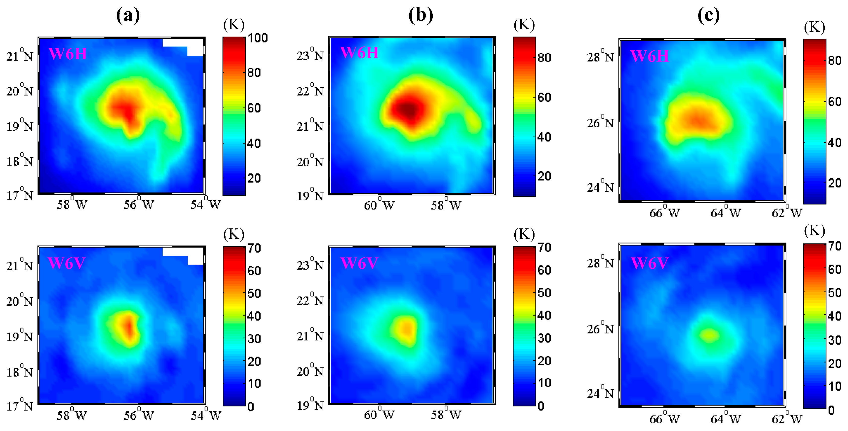
2.1. Microwave Brightness Temperature Data

The Advanced Microwave Scanning Radiometer–Earth Observing System (AMSR-E) sensor on NASA’s Aqua satellite is a conically scanning passive microwave instrument that provides measurements of the atmospheric and oceanic parameters for the investigation of global water and energy cycles. The AMSR-E instrument was launched on 2 May 2002, and ceased operations on 4 December 2011. Temporal coverage for the available data is from June 2002 to October 2011. The AMSR-E provides dual polarization observations (vertical and horizontal polarization) at frequencies ranging from 6.9 to 89 GHz. The integrated field of view (3-dB footprint size) is 75 × 43 km, 51 × 29 km, 27 × 16 km, 32 × 18 km, 14 × 8 km, and 7 × 4 km for 6.9, 10.65, 18.7, 23.8, 36.5, and 89.0 GHz, respectively. During a scan period of 1.5 s, the AMSR-E obtains data over a 1670-km swath. The nadir angle for the parabolic reflector is fixed at 47.4°, which results in an Earth incidence angle of approximately 55°.

2.2. H*Wind Analysis Data

Relatively reliable and reasonable estimates of TC wind speeds can be obtained from the H*wind analysis system [21]. This system provides an objective analysis of wind speed in TCs by assimilating all available wind measurements, such as ships, buoys, coastal platforms, surface-aviation reports, and some remote sensing data. All data are quality controlled and then processed to conform to a common framework for a 1-min sustained-wind field at a 10-m height above the sea surface [21]. Typical wind speed errors in an H*wind analysis are estimated to be 10% to 20% [22]. The wind speed errors will vary because of the quantity and quality of data that are available as well as the degree of quality control of this system. Although each wind speed analysis produced by this system may be inaccurate, the ensemble average over many collocations can minimize the error of the overall analysis. The H*wind analysis data are produced with a resolution of approximately 5 km and are available from the NOAA HRD.

2.3. Airborne SFMR Measurements

The stepped-frequency microwave radiometer (SFMR) is an airborne remote sensing instrument for measuring surface winds in TCs [2]. The SFMR observes TC at 6 frequencies, 4.55, 5.06, 5.64, 6.34, 6.96, and 7.22 GHz, and it provides along-track wind measurements up to 70 m/s [23]. Its spatial and temporal resolutions are 1.5 km and 1 s, respectively. The previous study [23] showed that the RMS error was approximately 4 m/s between the SFMR wind speeds and the Global Positioning System (GPS) dropwindsonde measurements for wind speeds ranging from 10 to 70 m/s. The accuracy of SFMR measurements was found to degrade at weaker wind speeds, particularly in heavy precipitation [24]. A revised set of geophysical model function (GMF) coefficients for both the rain absorption and wind-induced surface emissivity model has been developed to improve this situation [24].

2.4. Data Collections

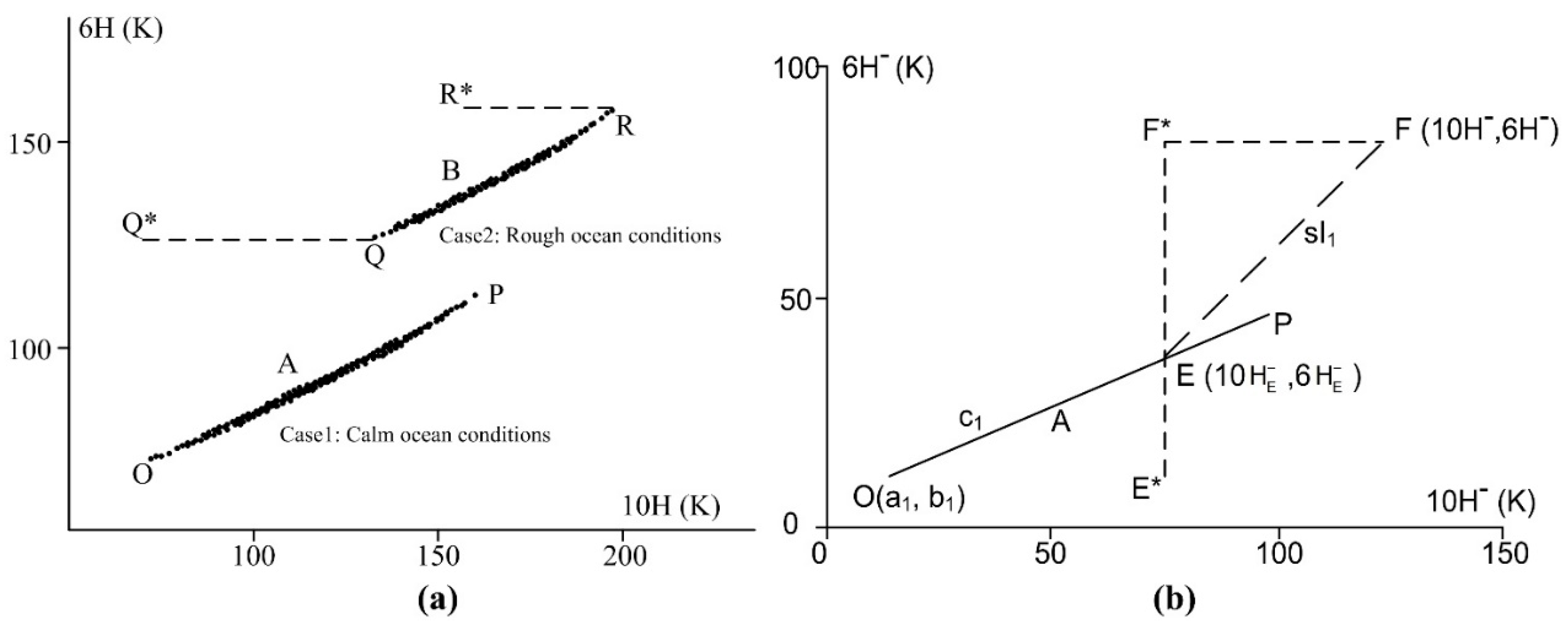
The selected microwave TB data are derived from AMSR-E. Correspondingly, the selected surface “true” winds are derived from the H*wind analysis system, which are used to produce the collocated data sets for training and testing the wind speed retrieval model in hurricanes.

To train and test the retrieval model, we collected data from 12 category 3–5 hurricanes from 2003 to 2011. To acquire a valid collocation, we required the time of the H*wind analysis data and the average time of the AMSR-E overpass to be within three hours. A hurricane can move a considerable distance within a three-hour time window [14]. Therefore, we shifted the H*wind analysis data for each hurricane referring to the “best track” information from the National Hurricane Center so that the eye of the H*wind analysis data coincided with the eye of the AMSR-E measurements. For each AMSR-E 6.9-GHz integrated field-of-view (IFOV), we found all the selected H*wind analyses on 5 km grids insides the AMSR-E 6.9-GHz IFOV and averaged these selected data using a Gaussian weighting based on the distance to the center of the IFOV [19]. In addition, we used a scale factor of 0.88 to convert from 1-min sustained H*wind analysis data to 10-min sustained satellite winds [25]. The statistics of collocation are presented in

Table 1. Statistics of matchups between AMSR-E measurements and H*wind analysis data.

Hurricane Name	Year	Max Winds (m/s)	AMSR-E–H*wind
			Population (≥18 m/s)	Longitude Shift (°)	Latitude Shift (°)
Fabian	2003	60	8919	0.044	0.110
Isabel	2003	73	6766	−0.205	0.107
Frances	2004	58	3452	−0.463	0.112
Ivan	2004	70	11,054	−0.260	0.103
Dennis	2005	65	2365	−0.149	0.110
Katrina	2005	75	2276	−0.020	0.025
Rita	2005	78	427	−0.318	−0.012
Bertha	2008	53	721	−0.064	0.198
Ike	2008	63	7087	−0.040	−0.037
Bill	2009	58	6381	−0.470	0.310
Igor	2010	68	7668	−0.321	0.199
Irene	2011	54	4749	−0.137	0.239

.

3. Method

Two new brightness temperature increments (W6H and W6V) from wind speeds inside hurricanes can be defined as

$$\mathrm{W}6\mathrm{H}=\frac{{\mathrm{EF}}^{*}}{{\mathrm{fac}}_1}=\frac{\left(6{\mathrm{H}}^{-}-6{\mathrm{H}}_{\mathrm{E}}^{-}\right)}{{\mathrm{fac}}_1}=\left(6{\mathrm{H}}^{-}-{\mathrm{c}}_1\times 10{\mathrm{H}}^{-}+{\mathrm{a}}_1\times {\mathrm{c}}_1-{\mathrm{b}}_1\right)\times \frac{{\mathrm{sl}}_1}{\left({\mathrm{sl}}_1-{\mathrm{c}}_1\right)}/{\mathrm{fac}}_1$$

(1)

$${\mathrm{sl}}_1={\mathrm{d}}_1+{\mathrm{e}}_1\times \left(10{\mathrm{H}}_{\mathrm{E}}^{-}-{\mathrm{a}}_1\right)$$

(2)

$${\mathrm{fac}}_1=1-{\mathrm{f}}_1\times \left(10{\mathrm{H}}_{\mathrm{E}}^{-}-{\mathrm{a}}_1\right)$$

(3)

$$6\left(10\right){\mathrm{H}}^{-}=\mathrm{AMSRE}\_6\left(10\right)\mathrm{H}-\mathrm{CalmOcean}\_6\left(10\right)\mathrm{H}$$

(4)

$$\mathrm{W}6\mathrm{V}=\frac{{\mathrm{EF}}^{*}}{{\mathrm{fac}}_2}=\frac{\left(6{\mathrm{V}}^{-}-6{\mathrm{V}}_{\mathrm{E}}^{-}\right)}{{\mathrm{fac}}_2}=\left(6{\mathrm{V}}^{-}-{\mathrm{c}}_2\times 10{\mathrm{V}}^{-}+{\mathrm{a}}_2\times {\mathrm{c}}_2-{\mathrm{b}}_2\right)\times \frac{{\mathrm{sl}}_2}{\left({\mathrm{sl}}_2-{\mathrm{c}}_2\right)}/{\mathrm{fac}}_2$$

(5)

$${\mathrm{sl}}_2={\mathrm{d}}_2+{\mathrm{e}}_2\times \left(10{\mathrm{V}}_{\mathrm{E}}^{-}-{\mathrm{a}}_2\right)$$

(6)

$${\mathrm{fac}}_2=1-{\mathrm{f}}_2\times \left(10{\mathrm{V}}_{\mathrm{E}}^{-}-{\mathrm{a}}_2\right)$$

(7)

$$6\left(10\right){\mathrm{V}}^{-}=\mathrm{AMSRE}\_6\left(10\right)\mathrm{V}-\mathrm{CalmOcean}\_6\left(10\right)\mathrm{V}$$

(8)

where the AMSRE_6(10)P is the AMSR-E measurement for the 6(10) GHz channel at P-polarization (P = H, V) and CalmOcean_6(10)P is the ocean emission for 6(10) GHz channel under calm ocean conditions. The definition of other parameters in Equations (1) to (8) can be found in Figure 1.

The simulated brightness temperature data of group A in Figure 1a are the results under calm ocean conditions. The brightness temperature increased from O to P because of the increments of water vapor and liquid water. The brightness temperature data of group B in Figure 1a are obtained by assuming a rough ocean condition. The point O under calm ocean condition shifts to Q under a rough ocean condition at the lowest atmospheric opacity, and point P shifts to R at the higher atmospheric opacity. In Figure 1a, the relationship between 6H and 10H is slightly nonlinear; however, we can approximate it as linear for simplicity. By calculating 6H⁻ and 10H, we can obtain Figure 1b in which line A is approximated as a linear line passing the point O(a₁, b₁) with slope c₁. Point F in Figure 1b corresponds to an arbitrary point on line B in Figure 1a. Then, we can obtain an intersecting point E made by the two lines OP and EF in Figure 1b. The slope of line EF is sl₁. Finally, we can obtain the parameter “W6H or W6V” (in degrees Kelvin) by the length of EF* divided by the atmospheric effect denoted by fac.

Finally, a wind speed retrieval model can be represented as

$$\begin{array}{cc}\mathrm{WS}={\mathrm{m}}_1\times \mathrm{W}6\mathrm{H}+{\mathrm{m}}_2\times \mathrm{W}6\mathrm{V}+{\mathrm{m}}_3& \mathrm{if}\mathrm{W}6\mathrm{H}<20\\ \mathrm{WS}={\mathrm{m}}_4\times \mathrm{W}6\mathrm{H}+{\mathrm{m}}_5\times \mathrm{W}6\mathrm{V}+{\mathrm{m}}_6& \mathrm{if}20\le \mathrm{W}6\mathrm{H}<30\\ \mathrm{WS}={\mathrm{m}}_7\times \mathrm{W}6\mathrm{H}+{\mathrm{m}}_8\times \mathrm{W}6\mathrm{V}+{\mathrm{m}}_9& \mathrm{if}\mathrm{W}6\mathrm{H}\ge 30\end{array}$$

(9)

where the unknown coefficients (a₁~f₁, a₂~f_2, and m₁~m₉) in Equations (1) to (9) can be derived from the matchups.

4. Results and Analysis

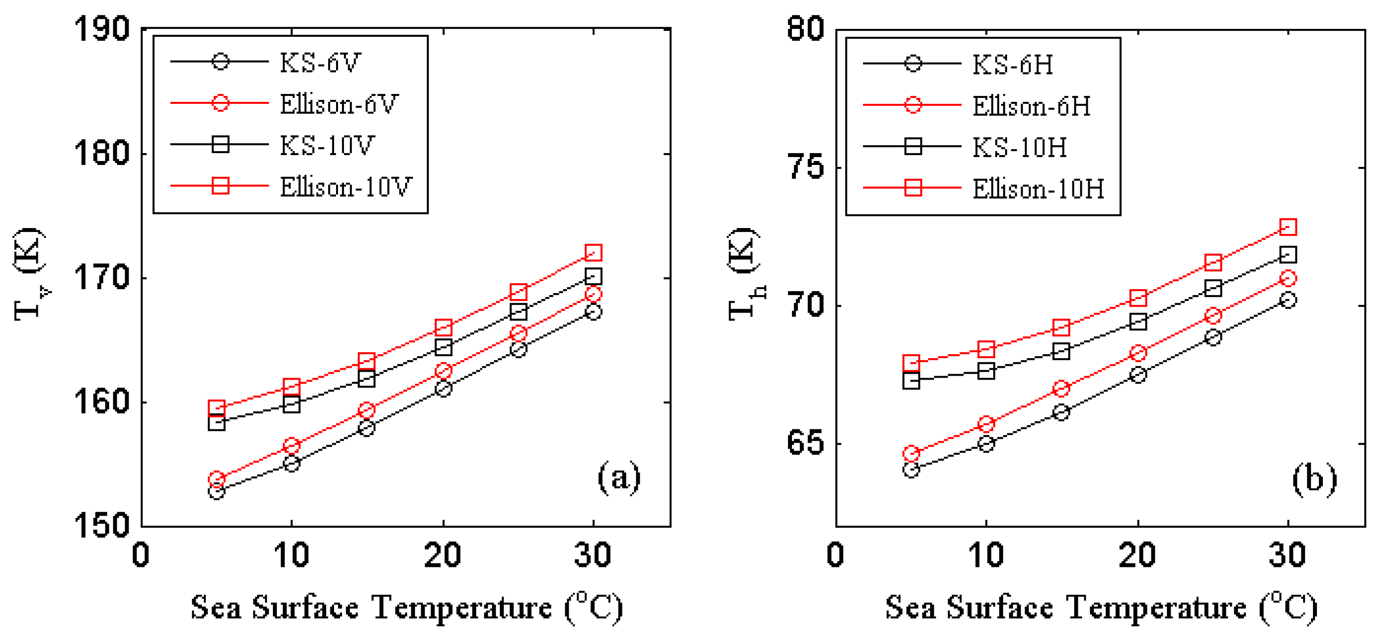
4.1. Comparison of the Klein-Swift Model and The Ellison Model

Before estimating the model coefficients, we need to calculate the parameter 6(10)P⁻ (P = V or H) with Equations (4) and (8). First, it need to estimate the calm ocean microwave emissions at both 6 and 10 GHz using Equations (10) and (11)

$$\mathrm{CalmOcean}\_6\left(10\right)\mathrm{H}=\mathrm{SST}\times \left[1-{\left|{\mathrm{R}}_{\mathrm{H}}\left(\mathsf{\theta }\right)\right|}^2\right]=\mathrm{SST}\times \left[1-{\left|\frac{\cos \mathsf{\theta }-\sqrt{{\mathsf{\epsilon }}_{\mathrm{r}}-{\sin }^2\mathsf{\theta }}}{\cos \mathsf{\theta }+\sqrt{{\mathsf{\epsilon }}_{\mathrm{r}}-{\sin }^2\mathsf{\theta }}}\right|}^2\right]$$

(10)

$$\mathrm{CalmOcean}\_6\left(10\right)\mathrm{V}=\mathrm{SST}\times \left[1-{\left|{\mathrm{R}}_{\mathrm{V}}\left(\mathsf{\theta }\right)\right|}^2\right]=\mathrm{SST}\times \left[1-{\left|\frac{{\mathsf{\epsilon }}_{\mathrm{r}}\cos \mathsf{\theta }-\sqrt{{\mathsf{\epsilon }}_{\mathrm{r}}-{\sin }^2\mathsf{\theta }}}{{\mathsf{\epsilon }}_{\mathrm{r}}\cos \mathsf{\theta }+\sqrt{{\mathsf{\epsilon }}_{\mathrm{r}}-{\sin }^2\mathsf{\theta }}}\right|}^2\right]$$

(11)

where θ is the Earth incidence angle and ${\epsilon }_r$ is the complex dielectric constant (permittivity) of sea water, which is a function of frequency, SST, and salinity. Some different permittivity models for pure water or sea water have been studied [26,27,28]. Two typical permittivity models were compared in calculating the calm ocean microwave emission: the Klein-Swift model [26] and the Ellison model [28]. The calculated brightness temperatures as a function of SST using the above models are displayed in Figure 2. The red curves are the calculation results of the Ellison model at different channels, and the black curves are the calculation results of the Klein-Swift model. From Figure 2, we can see that the results calculated using the Ellison model are higher than those using the Klein-Swift model. For h-pol, the calculated brightness temperature biases between the Ellison and Klein-Swift models increase with increasing SST; the biases are approximately 0.6 K (5 °C, at 6 GHz), 0.8 K (30 °C, at 6 GHz), 0.7 K (5 °C, at 10 GHz), and 1 K (30 °C, at 10 GHz). Similar results can be found at v-pol channels (Figure 2).

As a case study, the Klein-Swift and Ellison models were used to retrieve wind speeds over some typical hurricanes using the algorithm described in Section 3. The experimental data were derived from the previous study [15]. The SSTs were derived from the Reynolds weekly analysis data [29]. Figure 3a and Figure 4a display the calculated results using the Ellison model for hurricanes Frances (2004) and Rita (2005), respectively. Figure 3b and Figure 4b are the corresponding calculated results using the Klein-Swift model for hurricanes Frances and Rita, respectively. The overall results show that the Klein-Swift model achieved smaller RMS differences for either hurricane Frances or hurricane Rita. The statistical results are displayed at the top of each sub-figure (Figure 3 and Figure 4). Similar results were also found in other hurricanes. Therefore, we finally selected the Klein-Swift model to calculate the calm ocean microwave emission in the wind speed retrieval model.

In practical application, SST is one of the necessary input parameters that has not been retrieved by the present algorithm. Therefore, we next accessed the influence of SST for retrieval accuracy using the above collocations.

One of the crucial factors for TC occurrence is warm seawater, typically above 26.5 °C [30]. We thus studied sea surface temperature changes from 27 to 30 °C. The calculation results can be found in

Table 2. Errors between H*wind analysis data and the retrieved wind speeds using the Klein-swift model with different fixed sea surface temperatures.

Hurricane Name	Hurricane Frances (2004)				Hurricane Rita (2005)
Sea Surface Temperature (°C)	27	28	29	30	27	28	29	30
Mean bias (m/s)	−0.03	−0.02	−0.02	−0.02	0.12	0.11	0.11	0.12
RMS difference (m/s)	2.74	2.73	2.70	2.77	1.81	1.80	1.78	1.81

. When SST is 29 °C, the retrieval model showed the smallest RMS difference. Figure 3c and Figure 4c show the calculation results using the fixed SST (29 °C) for hurricanes Frances and Rita, respectively. The RMS difference using the fixed SST (29 °C) was slightly increased when compared with the calculation results using the Reynolds weekly analysis data (Figure 3b and Figure 4b). SST was not retrieved by the present retrieval algorithm. Therefore, we set SST as a constant (29 °C) in the wind speed retrieval model for better practical application.

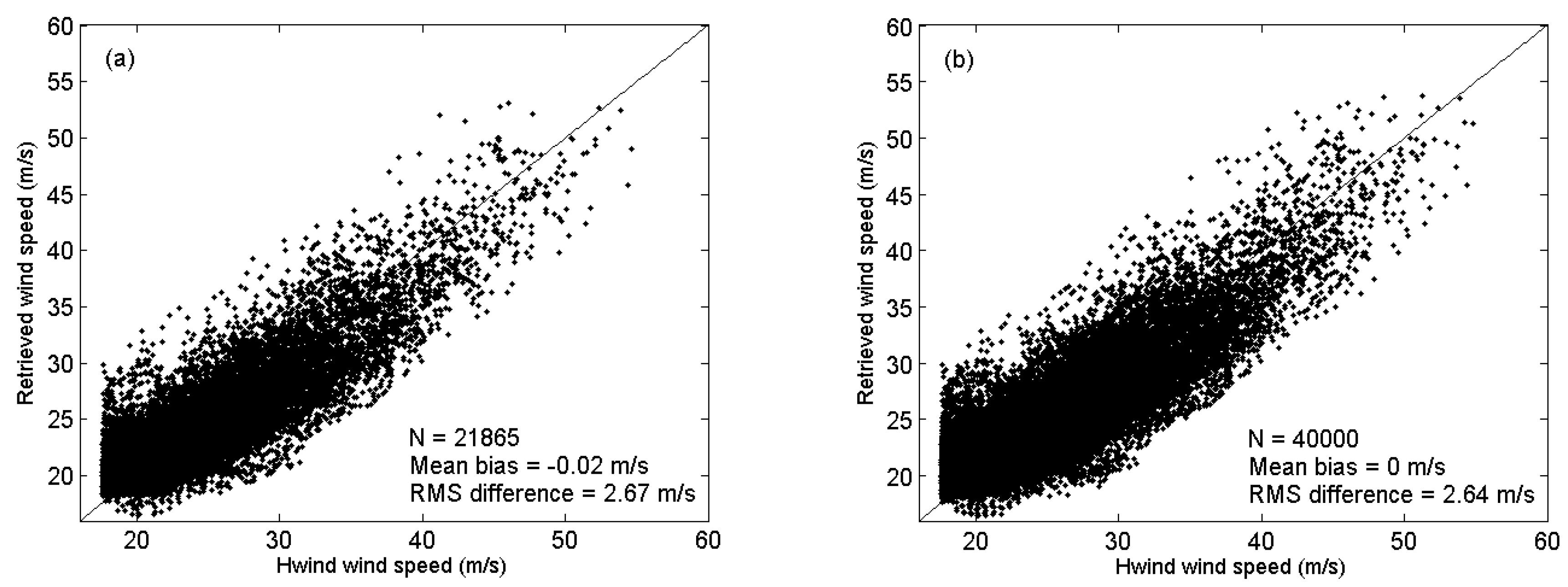
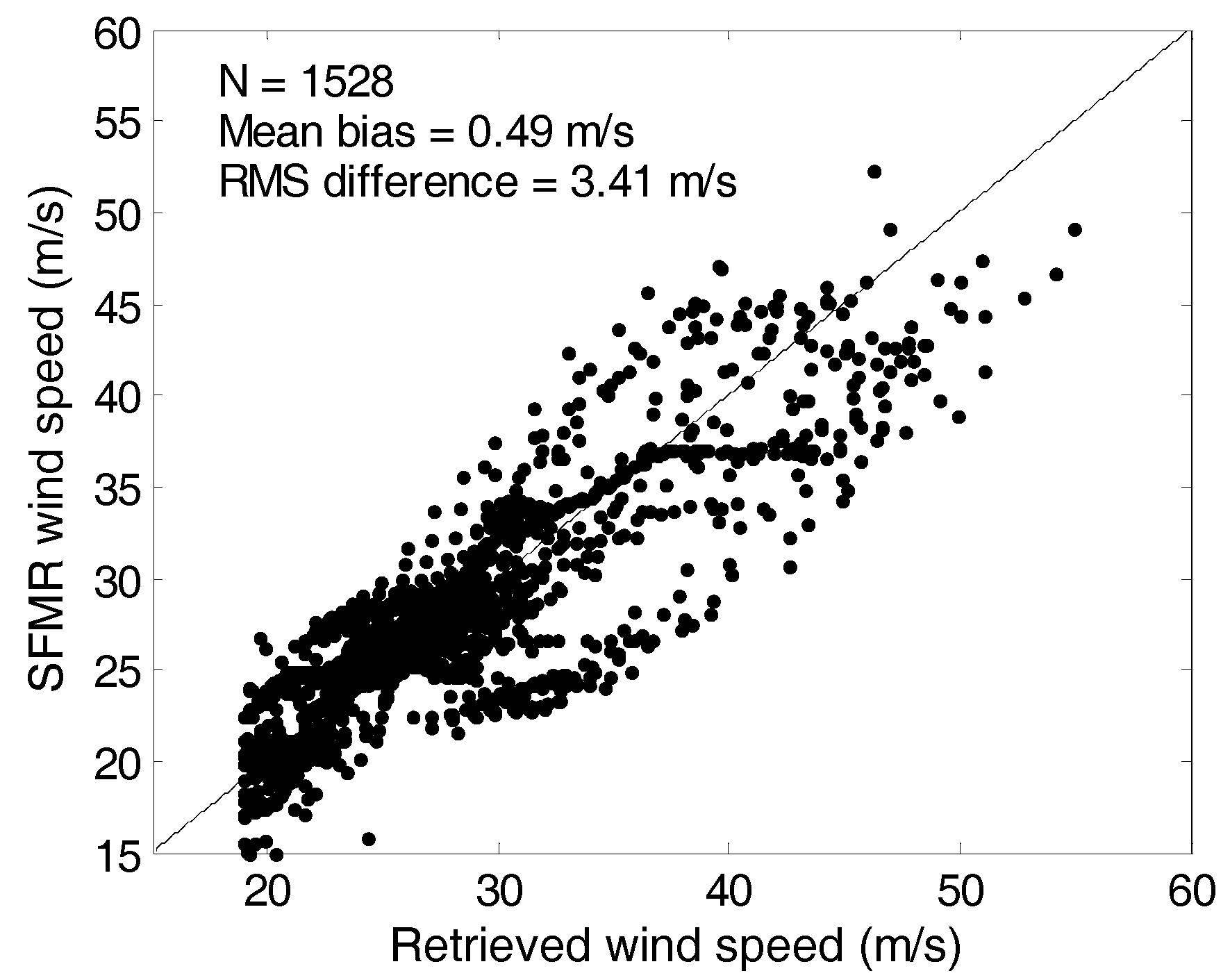
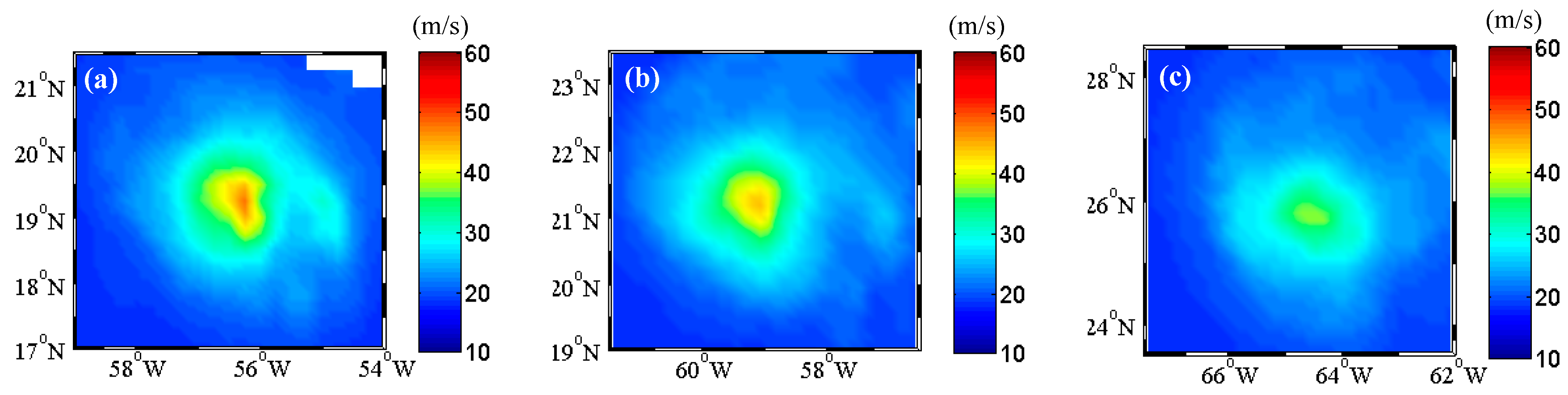
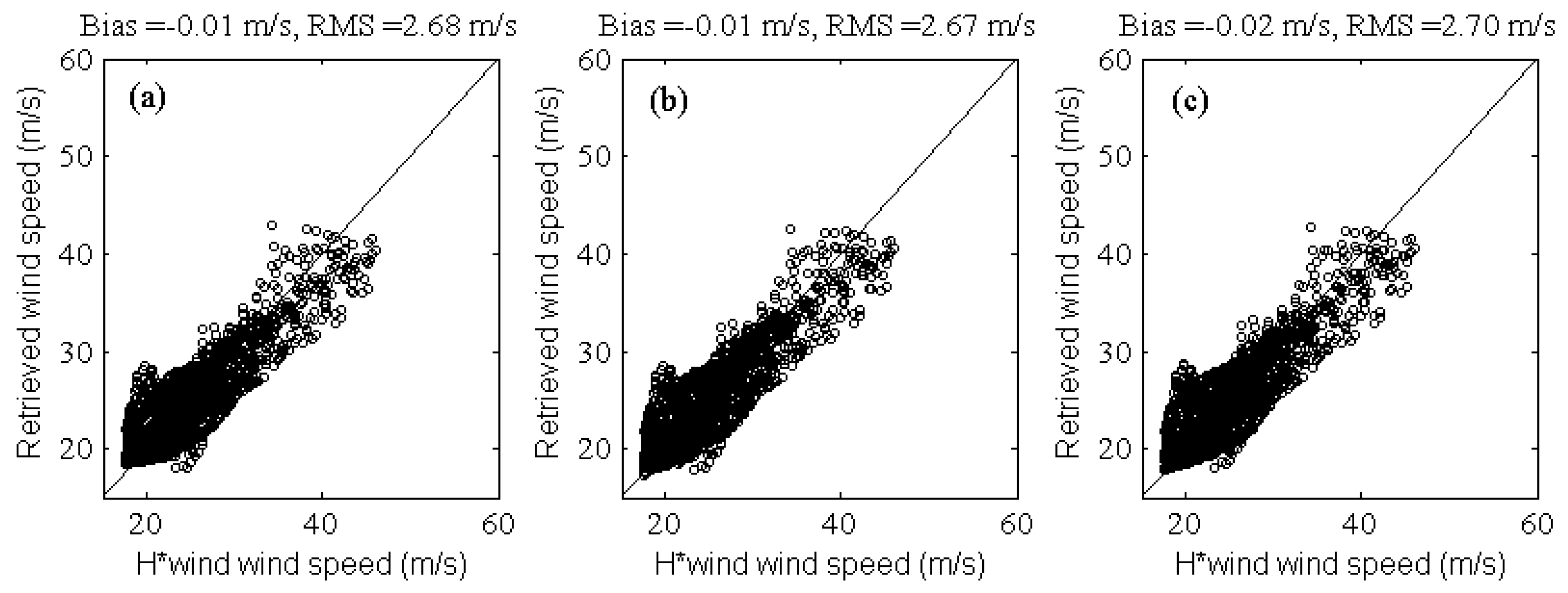
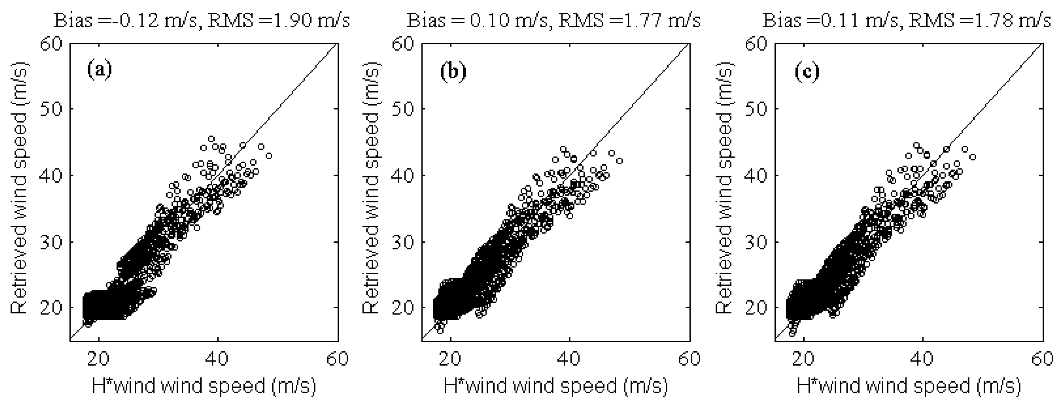
4.2. Wind Speed Retrieval and Validation for AMSR-E

The Earth incidence angles of AMSR-E at the 6 and 10 GHz channels were obviously different from those of WindSat. Therefore, we need to derive new wind speed retrieval model coefficients for the AMSR-E measurements. In this study, the AMSR-E brightness temperature data were collected at the 6 and 10 GHz v-pol and h-pol overpasses of 12 category 3–5 hurricanes between 2003 and 2011. The whole data set comprises 61,865 collocations. The collocations have been randomly divided into testing sets and validation sets. 21,865 observations are used for algorithm testing, and the other 40,000 observations are used for algorithm validation. The model coefficients in Equations (1) to (9) are listed in

Table 3. Model coefficients in Equations (1) to (9).

a1	b1	c1	d1	e1	f1
16.9925	5.5757	0.1201	0.8826	0.0153	0.0007
a2	b2	c2	d2	e2	f2
13.9971	5.6516	0.5158	0.8193	0.0012	0.0005
m1	m2	m3	m4	m5	m6
0.0050	0.0182	18.0131	0.2087	0.1588	12.0432
m7	m8	m9
0.1536	0.4107	10.6057

. The testing and validation results are shown in Figure 5. The mean bias and RMS difference are given in the top of each single panel. For wind speeds above 18 m/s, the mean bias and overall RMS difference of the new wind speed retrieval model for AMSR-E measurements were −0.01 m/s and 2.66 m/s, respectively. The mean bias (satellite-retrieved) was negative, which means that the AMSR-E retrieval model slightly overestimated wind speed.

In addition to the H*wind analysis data, we collected SFMR measurements to further validate the AMSR-E retrieved wind speeds, although the SFMR could only provide point observations along the aircraft flight track. A 15-km spatial window and 25-min temporal window were used to create the collocations. Finally, we obtained 1528 wind speed matchups for the selected 12 hurricanes. The collocations resulted in a mean bias of 0.49 m/s and an RMS difference of 3.41 m/s, shown in Figure 6. Overall, the AMSR-E retrieved wind speeds were larger than those from the SFMR.

As a case study, continuous monitoring of hurricane Bill was captured by AMSR-E measurements from 19 August 2009 to 21 August 2009. The evolution of brightness temperatures, including 6 GHz h-pol, 6 GHz v-pol, 10 GHz h-pol, 10 GHz v-pol, and rain rates are shown in Figure 7. The hurricane Bill rain rates were derived from AMSR-E measurements by Remote Sensing Systems (http://www.remss.com/). The rain bands in Figure 7 (bottom) matched well with the distributions of the selected low-frequency channel brightness temperature data (Figure 7) for regions outside of the eyewall. The corresponding brightness temperature increments of W6H are shown in Figure 8 (top) and were calculated with Equations (1) to (4). Figure 8 (bottom) shows the calculation results of the brightness temperature increments of W6V, which were calculated with Equations (5) to (8). Compared with the observed low-frequency brightness temperatures in Figure 7, the two new brightness temperature increments (Figure 8) can reduce the influence of rain to some extent.

Figure 9 shows the comparison of radiance characteristics for rain area and non-rain area over hurricane Bill on 19 August 2009, at 0512 to 0516 UTC. These results were used for quantitative analyses of rain effects on brightness temperature. Rain not only increased the observed brightness temperatures (Figure 9a) but also increased the brightness temperature increments of W6H and W6V (Figure 9b). The brightness temperature differences caused by rain are shown in Figure 9c. It can be seen that rain had different effects on different channels, which is obvious at higher frequencies (10 GHz). For horizontal polarization, the brightness temperature increment of W6H showed less sensitivity to rain than the observed 6 and 10 GHz h-pol brightness temperatures. Similarly, the brightness temperature increment of W6V showed the same characteristics. Therefore, the two brightness temperature increments of W6V and W6H appeared to be more suitable for retrieving wind speed than the observed low-frequency channel brightness temperatures. The same conclusion can also be made from Figure 10 and Figure 11.

Figure 12 shows the wind speed retrieval results of hurricane Bill over three continuous days (19–21 August). The sequence of figures clearly shows the intensification process of hurricane Bill.

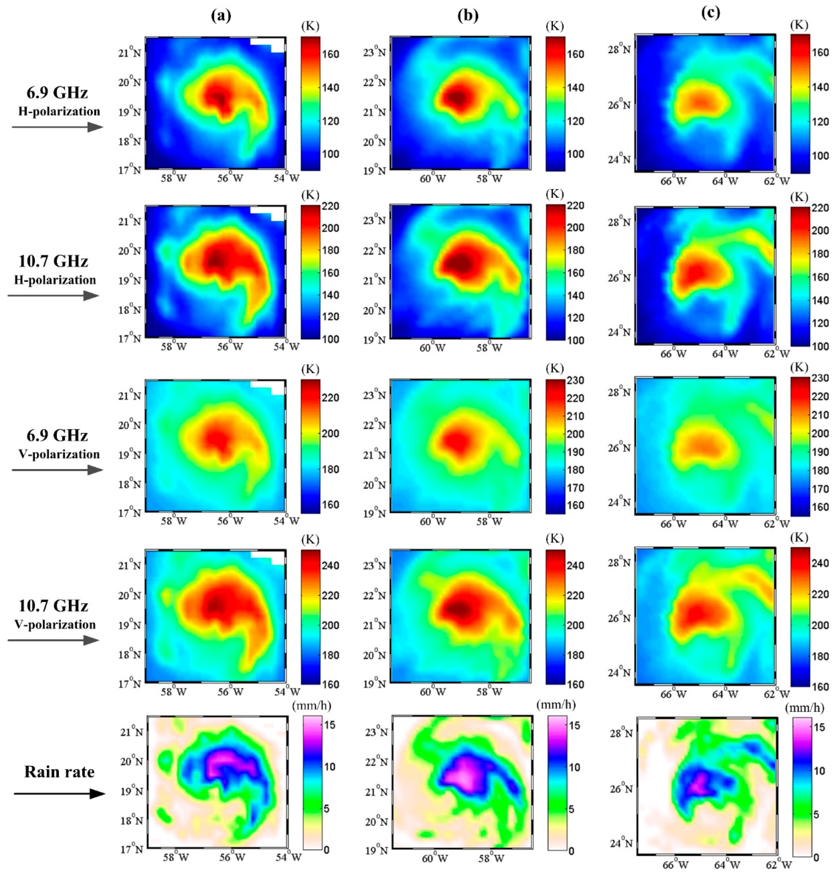
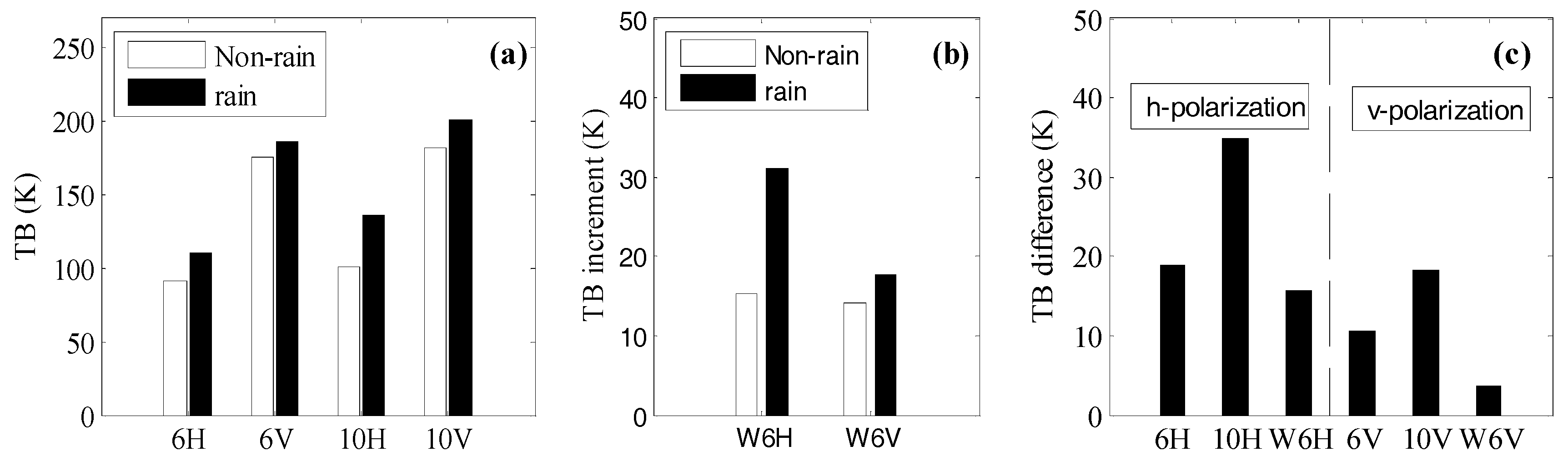
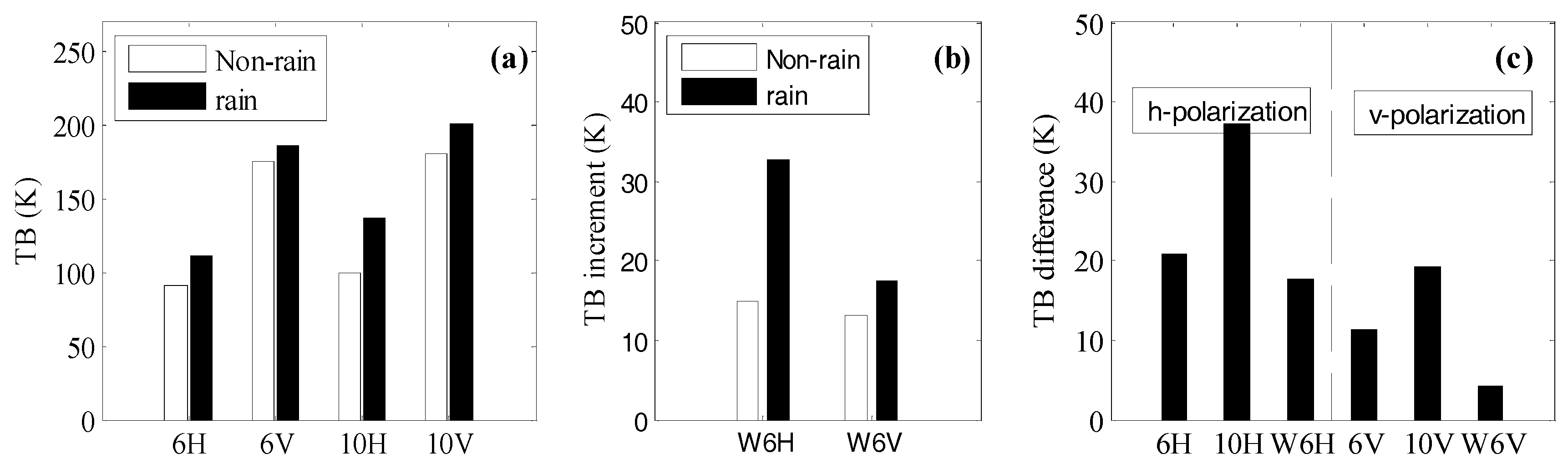
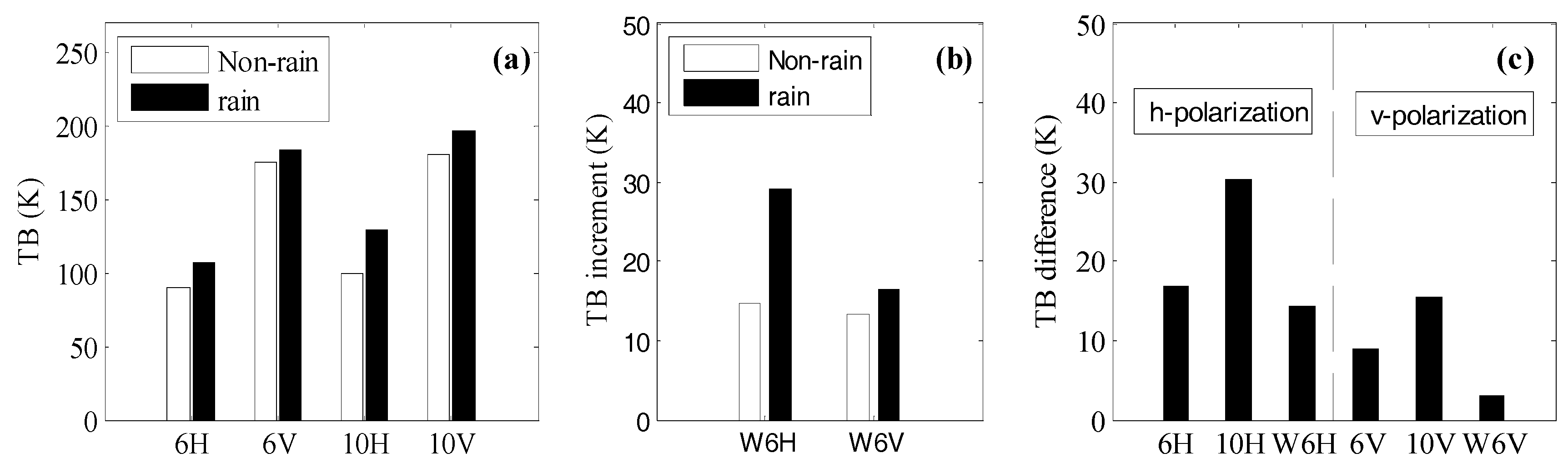
4.3. Rain Effects on Wind Retrieval

Rain is known to both attenuate and backscatter microwave signals. Brightness temperature acquired at higher frequencies (e.g., 36.5 GHz) saturates quickly and then decreases for most of the rainfall range. Brightness temperatures acquired at low frequencies, such as 6.9 and 10.7 GHz, are less sensitive to atmosphere and rain. Therefore, we could use the low-frequency channel brightness temperatures to retrieve wind speed under severe weather conditions, especially for typhoons and hurricanes.

As the rain rate increases, the space-borne microwave radiometer sees less and less of the radiation emitted by the surface and increasingly sees the radiation emitted by the rainy atmosphere. Therefore, it is very difficult to accurately model the brightness temperature in rainy atmospheres, especially given the high variability of rainy atmospheres. The brightness temperatures depend on cloud type and the distribution of rain within the footprint [31]. Therefore, the full Mie absorption theory needs to be applied when calculating the atmospheric radiative transfer equation. This requires additional input information such as the form and size of rain drops; however, these parameters are not readily available. In addition to these effects, there is a “splashing” effect. Rain changes the sea surface roughness in a complicated manner. Therefore, the statistical algorithm is a relatively suitable candidate for retrieving wind speed under severe weather conditions.

For the AMSR-E wind speed retrieval model, the effect of rain was determined using the AMSR-E rain rates from RSS.

Table 4. Statistics for different rain intervals between H*wind analysis data and the retrieved wind speed using AMSR-E measurements.

Rain Interval (mm/h)	Average Rain Rate (mm/h)	Number	Mean Bias (m/s)	RMSD (m/s)
[0, 2]	0.56	26193	−0.04	1.98
[2, 4]	2.98	8031	0.20	2.49
[4, 6]	5.05	7364	−0.15	2.70
[6, 8]	7.04	6761	−0.17	2.94
[8, 10]	9.02	5648	−0.09	3.19
[10, 12]	10.98	4226	−0.34	3.49
[12, 14]	12.93	2736	−0.12	3.65
Above 14	14.63	916	0.15	3.72

shows the biases and RMS difference between the retrieved wind speeds and the corresponding H*wind analysis wind speeds as a function of the AMSR-E rain rate. In general, the retrieved wind speed underestimated wind speed when the rain rate was less than 14 mm/h. The wind speed retrieval errors increased with the increasing AMSR-E rain rate.

5. Conclusions

In this study, two new brightness temperature increments were defined. One case study showed that the two brightness temperature increments were less sensitive to the rain than the observed C-band and X-band brightness temperature data. A new wind speed retrieval model was developed using the AMSR-E measurements.

Before developing the wind speed retrieval model, we need to estimate the calm ocean microwave emission at lower frequencies. Two typical permittivity models (Klein-Swift and Ellison) were tested to retrieve wind speeds inside hurricanes Frances (2004) and Rita (2005). Comparison showed that the Klein-Swift model achieved better results for hurricanes Frances and Rita. Additionally, SST was one of the necessary input parameters for calculating the calm ocean microwave emission and had not been retrieved in the present algorithm. Therefore, we compared the calculation results using the Reynolds weekly analysis data to those using a fixed SST. Finally, we used a fixed SST (29 °C) in the wind speed retrieval models, even if it was slightly worse than the retrieval results using the Reynolds weekly analysis data.

We used the AMSR-E measurements of 12 category 3–5 hurricanes between 2003 and 2011 and the corresponding H*wind analysis data to develop and validate the AMSR-E wind speed retrieval model. The retrieval model showed an encouraging performance for retrieving wind speeds inside hurricanes when compared with the corresponding H*wind analysis data; the mean bias was −0.01 m/s, and the RMS difference was 2.66 m/s. Good agreement was found between them. The SFMR measurements were used to further validate the AMSR-E retrieved wind speeds; the mean bias was 0.49 m/s, and the RMS difference was 3.41 m/s. One case study showed that the AMSR-E-retrieved wind speeds clearly illustrated the intensification process of hurricane Bill on 19–21 August 2009.

The new wind speed retrieval model can be used to retrieve wind speeds inside hurricanes with an encouraging degree of accuracy, although we cannot expect the models to have the same accuracy as in rain-free cases.

References

1. Jones, W.L.; Black, P.G.; Delnore, V.E.; Swift, C.T. Airborne microwave remote-sensing measurements of hurricane Allen. Science 1981, 214, 274–280. [Google Scholar] [CrossRef] [PubMed]
2. Uhlhorn, E.W.; Black, P.G. Verification of remotely sensed sea surface winds in hurricanes. J. Atmos. Ocean. Technol. 2003, 20, 99–116. [Google Scholar] [CrossRef]
3. Yueh, S.; Stiles, B.W.; Liu, W.T. QuikSCAT wind retrievals for tropical cyclones. IEEE Trans. Geosci. Remote Sens. 2003, 41, 2616–2628. [Google Scholar] [CrossRef]
4. Williams, B.A.; Long, D.G. Estimation of hurricane winds from SeaWinds at ultrahigh resolution. IEEE Trans. Geosci. Remote Sens. 2008, 46, 2924–2935. [Google Scholar] [CrossRef]
5. Stiles, B.W.; Dunbar, R.S. A neural network technique for improving the accuracy of scatterometer winds in rainy conditions. IEEE Trans. Geosci. Remote Sens. 2010, 48, 3114–3122. [Google Scholar] [CrossRef]
6. Zabolotskikh, E.; Mitnik, L.; Chapron, B. GCOM-W1 AMSR2 and MetOp-A ASCAT wind speeds for the extratropical cyclones over the North Atlantic. Remote Sens. Environ. 2014, 147, 89–98. [Google Scholar] [CrossRef]
7. Fernandez, D.; Carswell, J.R.; Frasier, S.; Chang, P.S.; Black, P.G.; Marks, F.D. Dual-polarized C- and Ku-band ocean backscatter response to hurricane-force winds. J. Geophys. Res. 2006, 111, C08013. [Google Scholar] [CrossRef]
8. Horstmann, J.; Thompson, D.R.; Monaldo, F.; Iris, S.; Graber, H.C. Can synthetic aperture radars be used to estimate hurricane force winds? Geophys. Res. Lett. 2005, 32, L22801. [Google Scholar] [CrossRef]
9. Shen, H.; Perrie, W.; He, Y. A new hurricane wind retrieval algorithm for SAR images. Geophys. Res. Lett. 2006, 33, L21812. [Google Scholar] [CrossRef]
10. Reppucci, A.; Lehner, S.; Schulz-Stellenfleth, J.; Yang, C.S. Extreme wind conditions observed by satellite synthetic aperture radar in the North West Pacific. Int. J. Remote Sens. 2008, 29, 6129–6144. [Google Scholar] [CrossRef]
11. Horstmann, J. Tropical cyclone winds from C-band cross-polarized synthetic aperture radar. IEEE Trans. Geosci. Remote Sens. 2015, 53, 2887–2898. [Google Scholar] [CrossRef]
12. Quilfen, Y.; Prigent, C.; Chapron, B. The potential of QuikSCAT and WindSat observations for the estimation of sea surface wind vector under severe weather conditions. J. Geophys. Res. 2007, 112, C09023. [Google Scholar] [CrossRef]
13. Shibata, A. A wind speed retrieval algorithm by combining 6 and 10 GHz data from advanced microwave scanning radiometer: Wind speed inside hurricanes. J. Oceanogr. 2006, 62, 351–359. [Google Scholar] [CrossRef]
14. Meissner, T.; Wentz, F.J. Wind vector retrievals under rain with passive satellite microwave radiometers. IEEE Trans. Geosci. Remote Sens. 2009, 47, 3065–3083. [Google Scholar] [CrossRef]
15. Zhang, L.; Yin, X.B.; Shi, H.Q.; Wang, Z.Z. Hurricane Wind Speed Estimation Using WindSat 6 and 10 GHz Brightness Temperatures. Remote Sens. 2016, 8, 721. [Google Scholar] [CrossRef]
16. Hong, S.; Seo, H.J.; Kwon, Y.J. A unique satellite-based sea surface wind speed algorithm and its application in tropical cyclone intensity analysis. J. Atmos. Ocean. Technol. 2016, 33, 1363–1375. [Google Scholar] [CrossRef]
17. Yan, B.; Weng, F. Applications of AMSR-E measurements for tropical cyclone predictions part I: Retrieval of sea surface temperature and wind speed. Adv. Atmos. Sci. 2008, 25, 227–245. [Google Scholar] [CrossRef]
18. Reul, N. SMOS satellite L-band radiometer: A new capability for ocean surface remote sensing in hurricanes. J. Geophys. Res. 2012, 117, C02006. [Google Scholar] [CrossRef]
19. Yueh, S. Directional signals in Windsat observations of hurricane ocean winds. IEEE Trans. Geosci. Remote Sens. 2008, 46, 130–136. [Google Scholar] [CrossRef]
20. Reul, N. A revised L-band radio-brightness sensitivity to extreme winds under Tropical Cyclones: The five year SMOS-storm database. Remote Sens. Environ. 2016, 180, 274–291. [Google Scholar] [CrossRef]
21. Powell, M.D.; Houston, S.H.; Amat, L.R. The HRD real-time hurricane wind analysis system. J. Wind Eng. Ind. Aerodyn. 1998, 77, 53–64. [Google Scholar] [CrossRef]
22. Houston, S.H.; Shaffer, W.A.; Powell, M.D. Comparisons of HRD and SLOSH surface wind fields in hurricanes: Implications for storm surge modeling. Weather Forecast. 1999, 14, 671–686. [Google Scholar] [CrossRef]
23. Uhlhorn, E.W. Hurricane surface wind measurements from an operational stepped frequency microwave radiometer. Mon. Weather Rev. 2007, 135, 3070–3085. [Google Scholar] [CrossRef]
24. Klotz, B.W.; Uhlhorn, E.W. Improved stepped frequency microwave radiometer tropical cyclone surface winds in heavy precipitation. J. Atmos. Ocean. Technol. 2014, 31, 2392–2408. [Google Scholar] [CrossRef]
25. Tropical Cyclone Forecasters’s Reference Guide. Available online: http://www.nrlmry.navy.mil/%7Echu/index.html (accessed on 11 March 2016).
26. Klein, L.A.; Swift, C.T. An improved model for the dielectric constant of sea water at microwave frequencies. IEEE J. Ocean. Eng. 1977, 2, 104–111. [Google Scholar] [CrossRef]
27. Liebe, H.J.; Hufford, G.A.; Manabe, T. A model for the complex permittivity of water at frequencies below 1 THz. Int. J. Infr. Millim. Waves 1991, 12, 659–675. [Google Scholar] [CrossRef]
28. Ellison, W. New permittivity measurements of seawater. Radio Sci. 1998, 33, 639–648. [Google Scholar] [CrossRef]
29. Reynolds, W.R.; Smith, T.M. Improved global sea surface temperature analyses using optimum interpolation. J. Clim. 1994, 7, 929–948. [Google Scholar] [CrossRef]
30. Webster, P.J.; Holland, G.J.; Curry, J.A. Changes in tropical cyclone number, duration, and intensity in a warming environment. Science 2005, 309, 1844–1846. [Google Scholar] [CrossRef] [PubMed]
31. Hilburn, K.A.; Wentz, F.J. Intercalibrated passive microwave rain products from the unified microwave ocean retrieval algorithm (UMORA). J. Appl. Meteorol. Climatol. 2008, 47, 778–794. [Google Scholar] [CrossRef]
Figure 1. (a) Brightness temperature data of 6H and 10H, group A for calm ocean conditions and group B for rough ocean conditions; (b) Thematic figure drawn from (a). The two figures can be found in [15].
Atmosphere 09 00034 g001
Figure 2. The calculated calm ocean brightness temperatures as a function of sea surface temperature using the Klein-Swift and Ellison models at 6 and 10 GHz channels: (a) v-pol; and (b) h-pol.
Atmosphere 09 00034 g002
Figure 3. H*wind analysis data versus the retrieved wind speeds over hurricane Frances (2004): (a) using the Ellison model and the Reynolds weekly analysis data; (b) using the Klein-Swift model and the Reynolds weekly analysis data; and (c) using the Klein-Swift model and a fixed SST (29 °C).
Atmosphere 09 00034 g003
Figure 4. H*wind analysis data versus the retrieved wind speeds over hurricane Rita (2005): (a) using the Ellison model and the Reynolds weekly analysis data; (b) using the Klein-Swift model and the Reynolds weekly analysis data; and (c) using the Klein-Swift model and a fixed SST (29 °C).
Atmosphere 09 00034 g004
Figure 5. Comparisons between H*wind analysis data and the retrieved wind speeds: (a) testing results; and (b) validation results.
Atmosphere 09 00034 g005
Figure 6. SFMR wind speed products versus the retrieved wind speeds using the AMSR-E 6 and 10 GHz brightness temperature data.
Atmosphere 09 00034 g006
Figure 7. AMSR-E observed low-frequency channel brightness temperatures and rain rates over hurricane Bill on (a) 19 August 2009, at 1650 to 1654 UTC; (b) 20 August 2009, at 0512 to 0516 UTC; and (c) 21 August 2009, at 0555 to 0559 UTC.
Atmosphere 09 00034 g007
Figure 8. Brightness temperature increments of W6H and W6V over hurricane Bill on (a) 19 August 2009, at 1650 to 1654 UTC; (b) 20 August 2009, at 0512 to 0516 UTC; and (c) 21 August 2009, at 0555 to 0559 UTC.
Atmosphere 09 00034 g008
Figure 9. Comparison of radiance characteristics for rain area and non-rain area over hurricane Bill on 19 August 2009, at 1650 to 1654 UTC. (a) Average brightness temperature value of each selected channel; (b) average brightness temperature increment of W6H (W6V); and (c) brightness temperature difference caused by rain.
Atmosphere 09 00034 g009
Figure 10. Comparison of radiance characteristics for rain area and non-rain area over hurricane Bill on 20 August 2009, at 0512 to 0516 UTC. (a) Average brightness temperature of each selected channel; (b) average brightness temperature increment of W6H (W6V); and (c) brightness temperature difference caused by rain.
Atmosphere 09 00034 g010
Figure 11. Comparison of radiance characteristics for rain area and non-rain area over hurricane Bill on 21 August 2009, at 0555 to 0559 UTC. (a) Average brightness temperature of each selected channel; (b) average brightness temperature increment of W6H (W6V); and (c) brightness temperature difference caused by rain.
Atmosphere 09 00034 g011
Figure 12. Retrieved wind speeds using the AMSR-E 6 and 10 GHz h-pol and v-pol brightness temperature data over hurricane Bill on (a) 19 August 2009, at 1650 to 1654 UTC; (b) 20 August 2009, at 0512 to 0516 UTC; and (c) 21 August 2009, at 0555 to 0559 UTC.
Atmosphere 09 00034 g012