Machine Learning to Predict the Global Distribution of Aerosol Mixing State Metrics


Abstract

1. Introduction
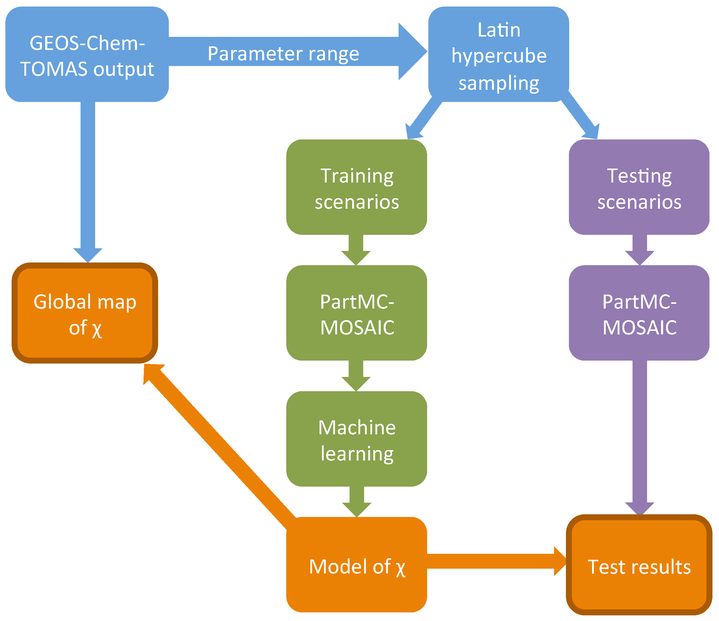
2. Methods
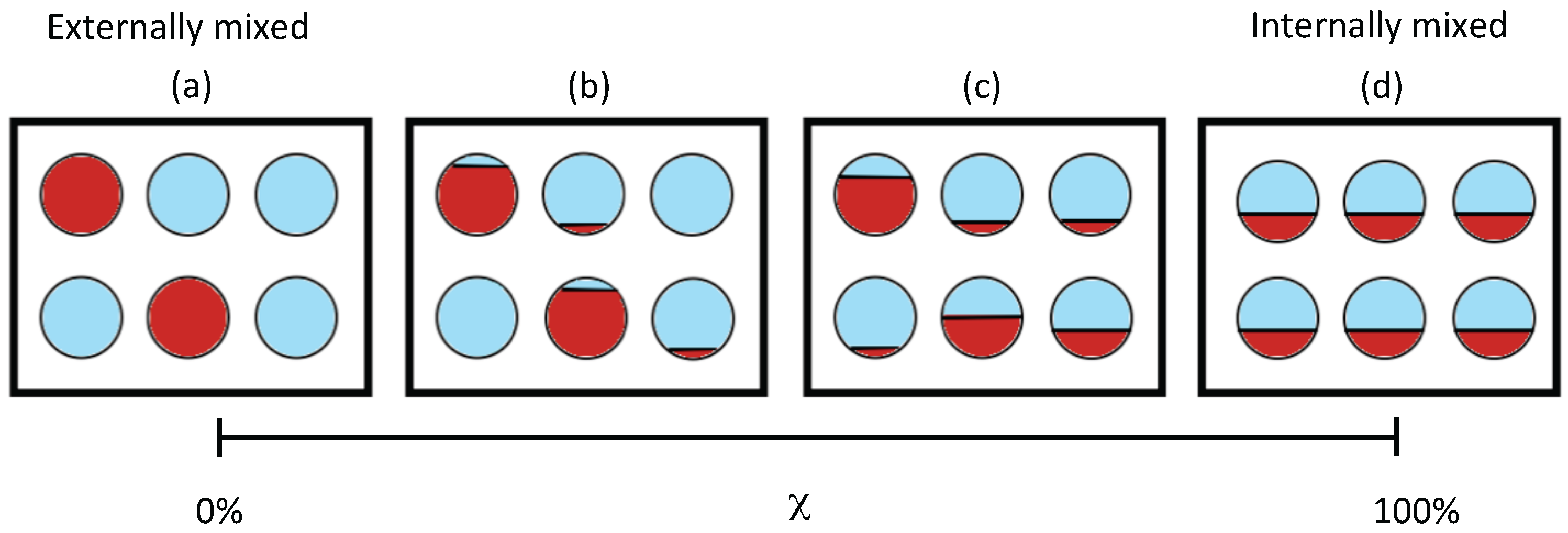
2.1. Mixing State Metric
2.2. Particle-Resolved Aerosol Modeling
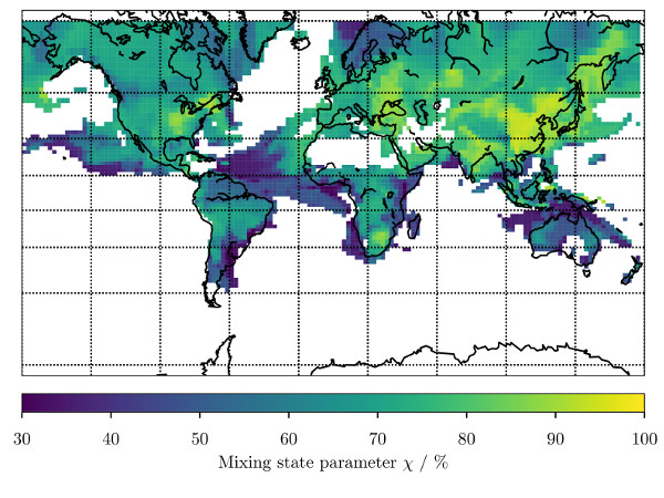
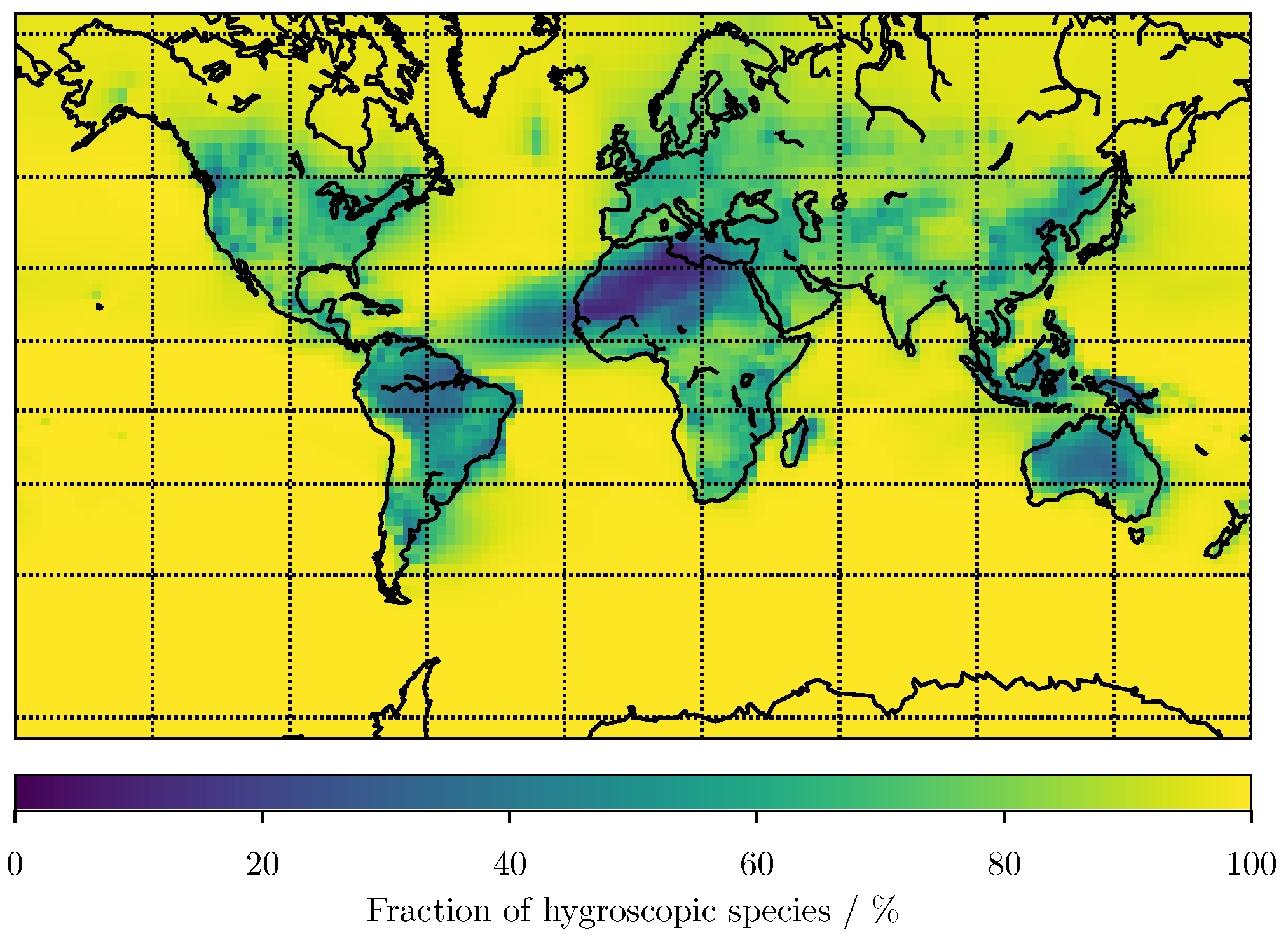
2.3. GEOS-Chem-TOMAS Dataset
2.4. Design of the Training and the Testing Scenarios
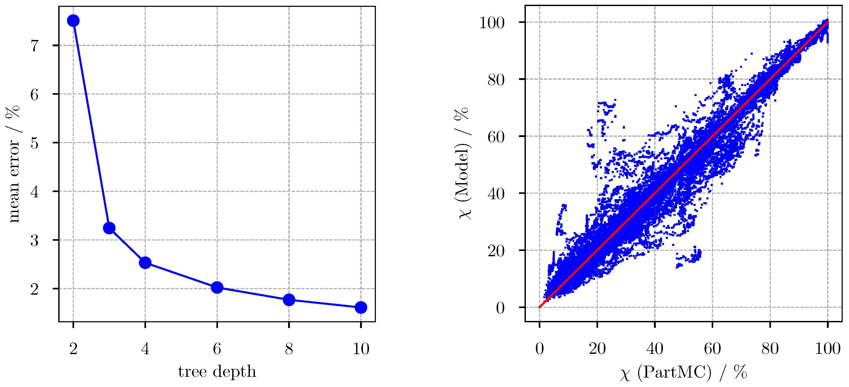
2.5. Machine Learning as Applied to PartMC
3. Results
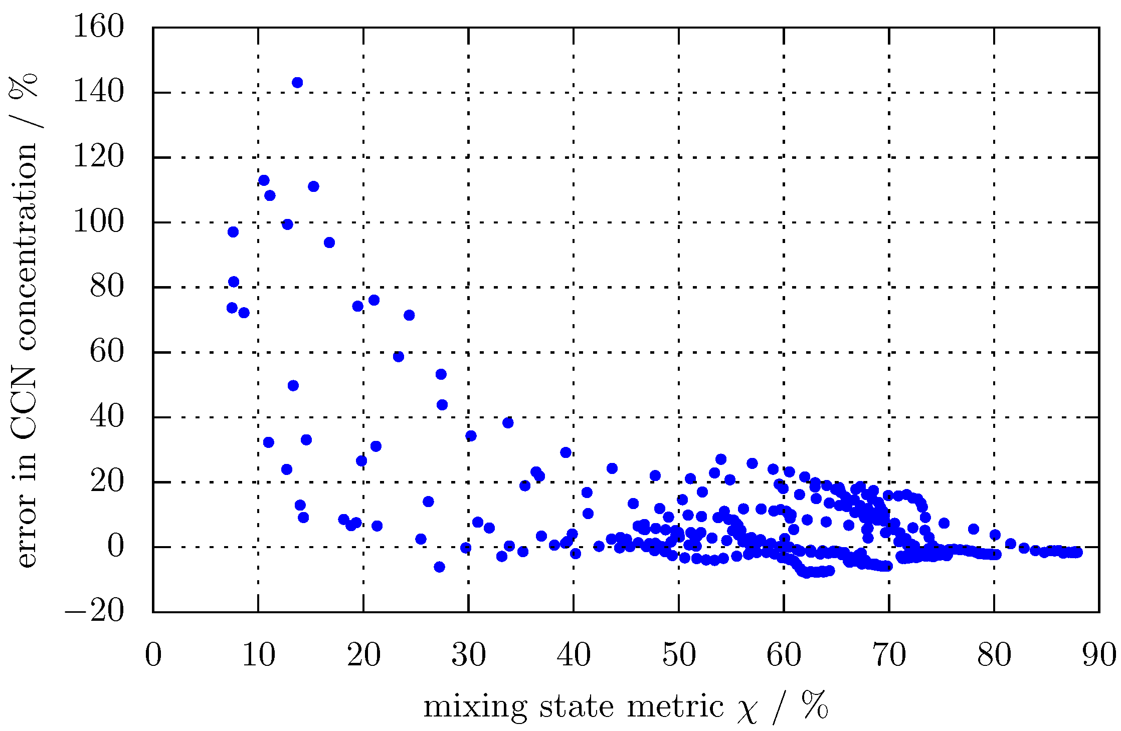
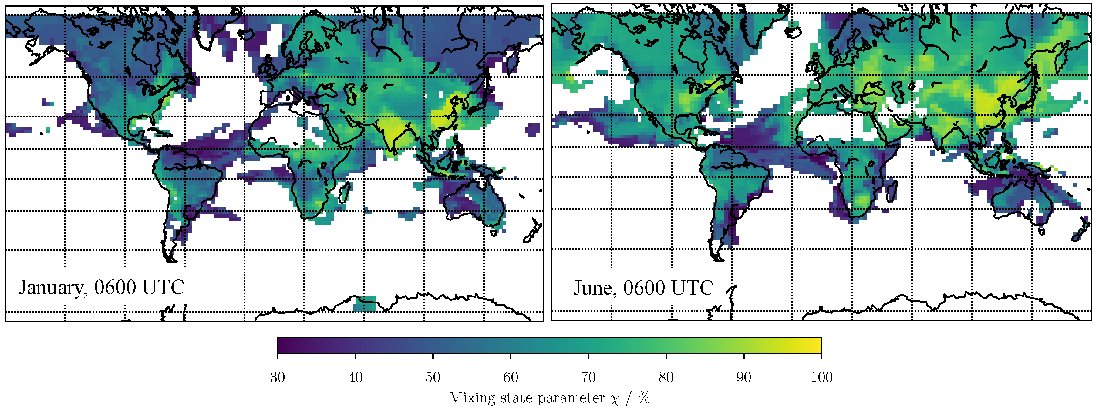
3.1. Predicting for the Bulk Aerosol Population
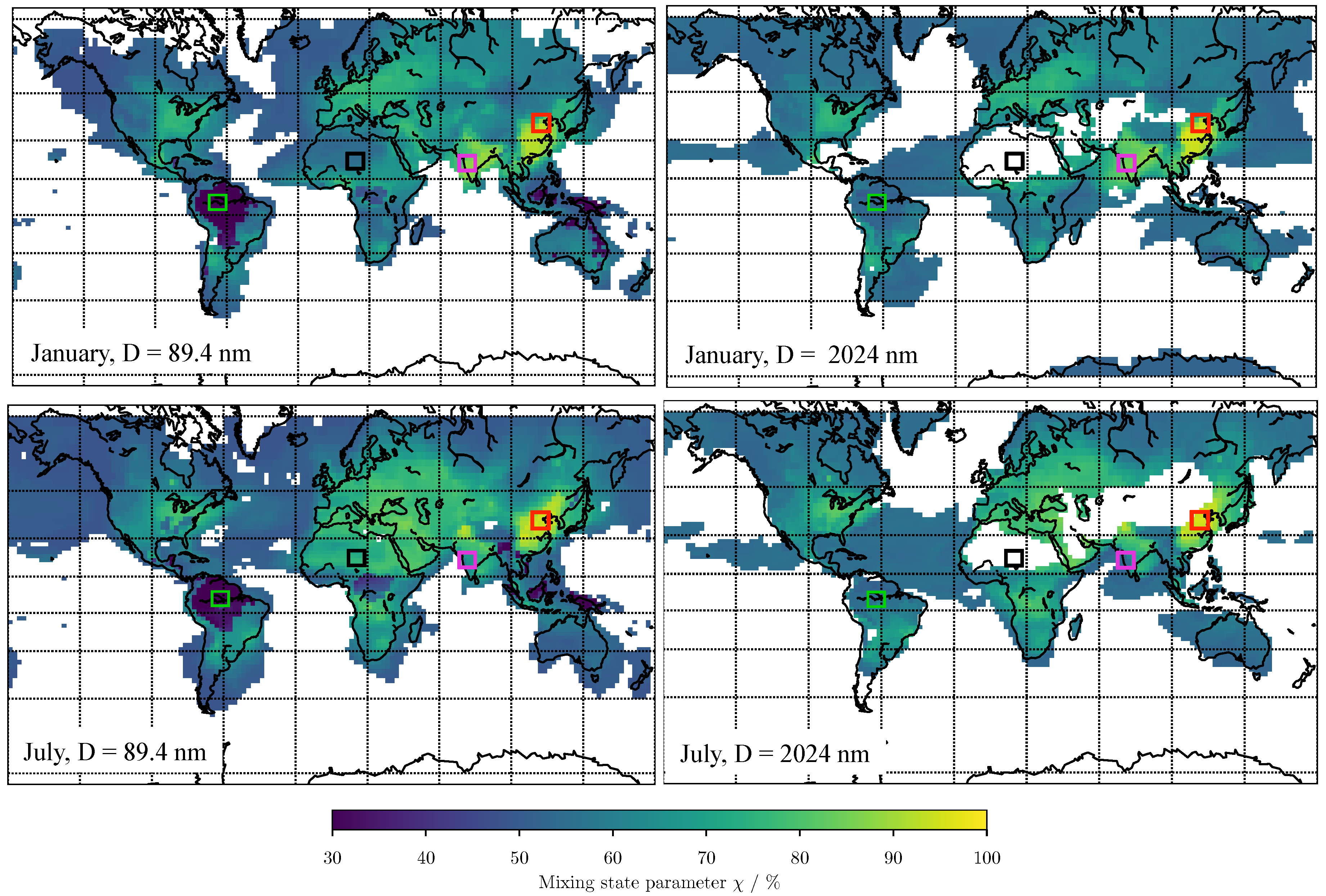
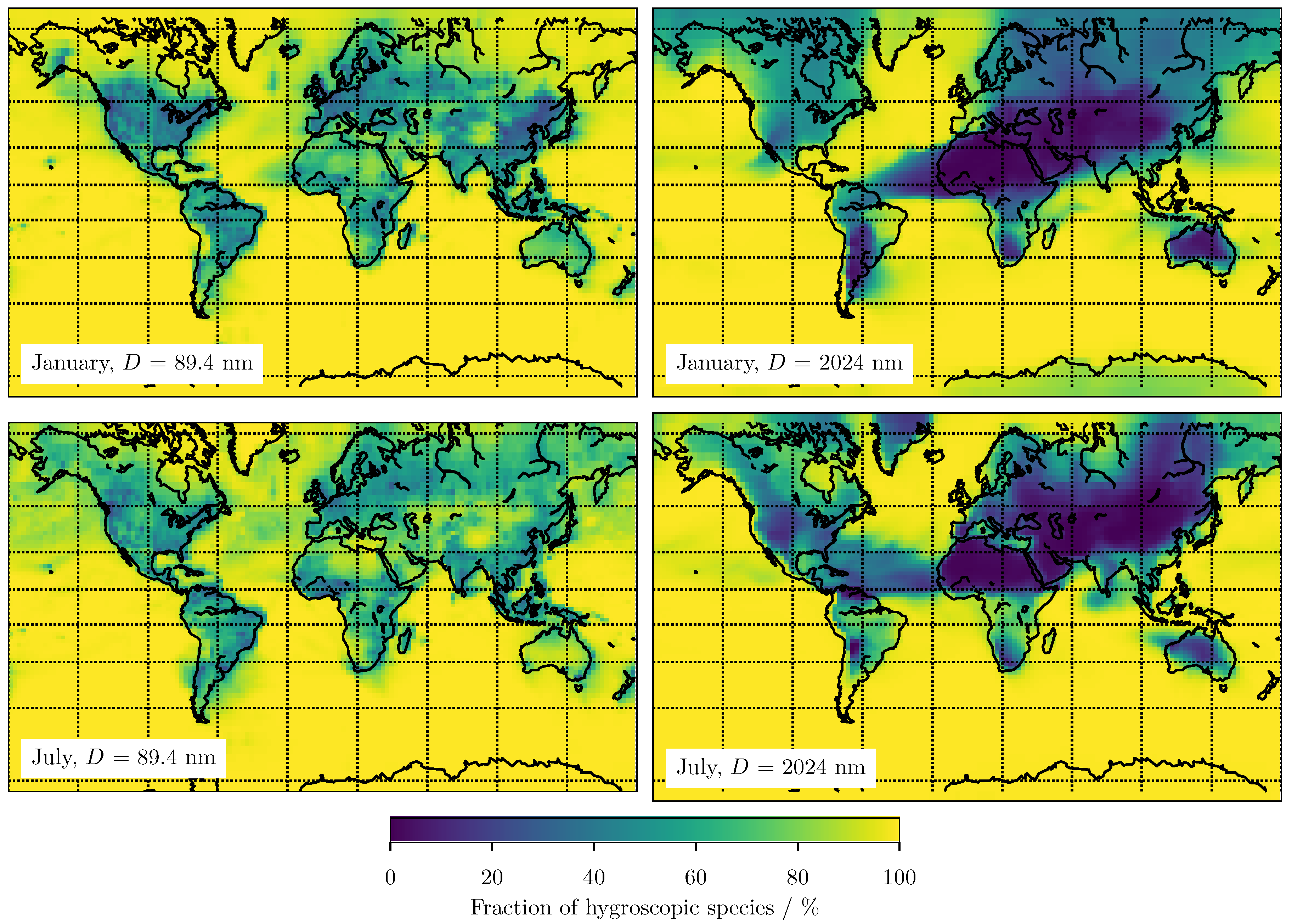
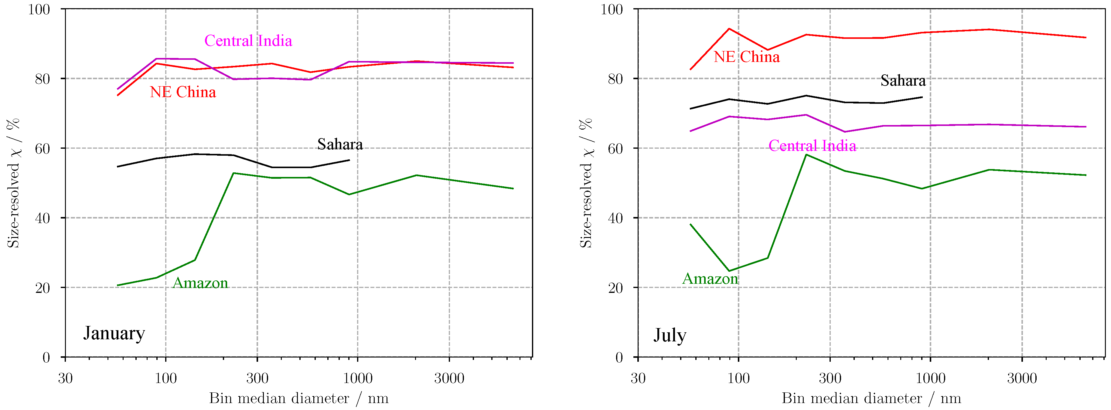
3.2. Predicting for Individual Size Bins
4. Conclusions
Acknowledgments
Author Contributions
Conflicts of Interest
References
- Noble, C.A.; Prather, K.A. Real-time single particle mass spectrometry: A historical review of a quarter century of the chemical analysis of aerosols. Mass Spectrom. Rev. 2000, 19, 248–274. [Google Scholar] [CrossRef]
- Bein, K.J.; Zhao, Y.; Wexler, A.S.; Johnston, M.V. Speciation of size-resolved individual ultrafine particles in Pittsburgh, Pennsylvania. J. Geophys. Res. 2005, 110, D07S05. [Google Scholar] [CrossRef]
- Johnson, K.S.; Zuberi, B.; Molina, L.T.; Molina, M.J.; Iedema, M.J.; Cowin, J.P.; Gaspar, D.J.; Wang, C.; Laskin, A. Processing of soot in an urban environment: Case study from the Mexico City Metropolitan Area. Atmos. Chem. Phys. 2005, 5, 3033–3043. [Google Scholar] [CrossRef]
- Riemer, N.; West, M.; Zaveri, R.; Easter, R. Simulating the evolution of soot mixing state with a particle-resolved aerosol model. J. Geophys. Res. Atmos. 2009, 114, D09202. [Google Scholar] [CrossRef]
- Seigneur, C.; Hudischewskyj, A.B.; Seinfeld, J.H.; Whitby, K.T.; Whitby, E.R.; Brock, J.R.; Barnes, H.M. Simulation of aerosol dynamics: A comparative review of mathematical models. Aerosol Sci. Technol. 1986, 5, 205–222. [Google Scholar] [CrossRef]
- Wexler, A.S.; Lurmann, F.W.; Seinfeld, J.H. Modelling urban aerosols—I. Model development. Atmos. Environ. 1994, 28, 531–546. [Google Scholar] [CrossRef]
- Whitby, E.R.; McMurry, P.H. Modal aerosol dynamics modeling. Aerosol Sci. Technol. 1997, 27, 673–688. [Google Scholar] [CrossRef]
- Zaveri, R.; Barnard, J.; Easter, R.; Riemer, N.; West, M. Effect of aerosol mixing-state on optical and cloud activation properties. J. Geophys. Res. Atmos. 2010, 115, D17210. [Google Scholar] [CrossRef]
- Fierce, L.; Riemer, N.; Bond, T.C. Toward reduced representation of mixing state for simulating aerosol effects on climate. Bull. Am. Meteorol. Soc. 2017, 98, 971–980. [Google Scholar] [CrossRef]
- Fierce, L.; Bond, T.C.; Bauer, S.E.; Mena, F.; Riemer, N. Black carbon absorption at the global scale is affected by particle-scale diversity in composition. Nat. Commun. 2016, 7, 12361. [Google Scholar] [CrossRef] [PubMed]
- Ching, J.; Riemer, N.; West, M. Impacts of black carbon mixing state on black carbon nucleation scavenging: Insights from a particle-resolved model. J. Geophys. Res. Atmos. 2012, 117. [Google Scholar] [CrossRef]
- Ching, J.; Riemer, N.; West, M. Impacts of black carbon particles mixing state on cloud microphysical properties: Sensitivity to environmental conditions. J. Geophys. Res. Atmos. 2016, 121, 5990–6013. [Google Scholar] [CrossRef]
- Riemer, N.; West, M. Quantifying aerosol mixing state with entropy and diversity measures. Atmos. Chem. Phys. 2013, 13, 11423–11439. [Google Scholar] [CrossRef]
- Ching, J.; Fast, J.; West, M.; Riemer, N. Metrics to quantify the importance of mixing state for CCN activity. Atmos. Chem. Phys. 2017, 17, 7445–7458. [Google Scholar] [CrossRef]
- Healy, R.; Riemer, N.; Wenger, J.; Murphy, M.; West, M.; Poulain, L.; Wiedensohler, A.; O’Connor, I.; McGillicuddy, E.; Sodeau, J.; et al. Single particle diversity and mixing state measurements. Atmos. Chem. Phys. 2014, 14, 6289–6299. [Google Scholar] [CrossRef]
- O’Brien, R.E.; Wang, B.; Laskin, A.; Riemer, N.; West, M.; Zhang, Q.; Sun, Y.; Yu, X.Y.; Alpert, P.; Knopf, D.A.; et al. Chemical imaging of ambient aerosol particles: Observational constraints on mixing state parameterization. J. Geophys. Res. 2015, 120, 9591–9605. [Google Scholar] [CrossRef]
- Adams, P.J.; Seinfeld, J.H. Predicting global aerosol size distributions in general circulation models. J. Geophys. Res. Atmos. 2002, 107, 4370. [Google Scholar] [CrossRef]
- Kodros, J.K.; Cucinotta, R.; Ridley, D.A.; Wiedinmyer, C.; Pierce, J.R. The aerosol radiative effects of uncontrolled combustion of domestic waste. Atmos. Chem. Phys. 2016, 16, 6771–6784. [Google Scholar] [CrossRef]
- Ghan, S.J.; Abdul-Razzak, H.; Nenes, A.; Ming, Y.; Liu, X.; Ovchinnikov, M.; Shipway, B.; Meskhidze, N.; Xu, J.; Shi, X. Droplet nucleation: Physically-based parameterizations and comparative evaluation. J. Adv. Model. Earth Syst. 2011, 3. [Google Scholar] [CrossRef]
- Whittaker, R.H. Evolution and Measurement of Species Diversity. Taxon 1972, 21, 213–251. [Google Scholar] [CrossRef]
- Drucker, J. Industrial Structure and the Sources of Agglomeration Economies: Evidence from Manufacturing Plant Production. Growth Chang. 2013, 44, 54–91. [Google Scholar] [CrossRef]
- Strong, S.; Koberle, R.; de Ruyter van Steveninck, R.; Bialek, W. Entropy and Information in Neural Spike Trains. Phys. Rev. Lett. 1998, 80, 197–200. [Google Scholar] [CrossRef]
- Falush, D.; Stephens, M.; Pritchard, J.K. Inference of population structure using multilocus genotype data: Dominant markers and null alleles. Mol. Ecol. Notes 2007, 7, 574–578. [Google Scholar] [CrossRef] [PubMed]
- Giorio, C.; Tapparo, A.; Dall’Osto, M.; Beddows, D.C.; Esser-Gietl, J.K.; Healy, R.M.; Harrison, R.M. Local and Regional Components of Aerosol in a Heavily Trafficked Street Canyon in Central London Derived from PMF and Cluster Analysis of Single-Particle ATOFMS Spectra. Environ. Sci. Technol. 2015, 49, 3330–3340. [Google Scholar] [CrossRef] [PubMed]
- Fraund, M.; Pham, D.Q.; Bonanno, D.; Harder, T.H.; Wang, B.; Brito, J.; de Sá, S.S.; Carbone, S.; China, S.; Artaxo, P.; et al. Elemental Mixing State of Aerosol Particles Collected in Central Amazonia during GoAmazon2014/15. Atmosphere 2017, 8, 173. [Google Scholar] [CrossRef]
- Dickau, M.; Olfert, J.; Stettler, M.E.J.; Boies, A.; Momenimovahed, A.; Thomson, K.; Smallwood, G.; Johnson, M. Methodology for quantifying the volatile mixing state of an aerosol. Aerosol Sci. Technol. 2016, 50, 759–772. [Google Scholar] [CrossRef]
- DeVille, R.E.L.; Riemer, N.; West, M. Weighted Flow Algorithms (WFA) for stochastic particle coagulation. J. Comput. Phys. 2011, 230, 8427–8451. [Google Scholar] [CrossRef]
- Michelotti, M.D.; Heath, M.T.; West, M. Binning for efficient stochastic multiscale particle simulations. Multiscale Model. Simul. 2013, 11, 1071–1096. [Google Scholar] [CrossRef]
- Zaveri, R.A.; Easter, R.C.; Fast, J.D.; Peters, L.K. Model for simulating aerosol interactions and chemistry (MOSAIC). J. Geophys. Res. Atmos. (1984–2012) 2008, 113. [Google Scholar] [CrossRef]
- Zaveri, R.A.; Peters, L.K. A new lumped structure photochemical mechanism for large-scale applications. J. Geophys. Res. Atmos. (1984–2012) 1999, 104, 30387–30415. [Google Scholar] [CrossRef]
- Zaveri, R.A.; Easter, R.C.; Wexler, A.S. A new method for multicomponent activity coefficients of electrolytes in aqueous atmospheric aerosols. J. Geophys. Res. Atmos. (1984–2012) 2005, 110. [Google Scholar] [CrossRef]
- Zaveri, R.A.; Easter, R.C.; Peters, L.K. A computationally efficient multicomponent equilibrium solver for aerosols (MESA). J. Geophys. Res. Atmos. (1984–2012) 2005, 110. [Google Scholar] [CrossRef]
- Schell, B.; Ackermann, I.J.; Binkowski, F.S.; Ebel, A. Modeling the formation of secondary organic aerosol within a comprehensive air quality model system. J. Geophys. Res. 2001, 106, 28275–28293. [Google Scholar] [CrossRef]
- Tian, J.; Riemer, N.; West, M.; Pfaffenberger, L.; Schlager, H.; Petzold, A. Modeling the evolution of aerosol particles in a ship plume using PartMC-MOSAIC. Atmos. Chem. Phys. 2014, 14, 5327–5347. [Google Scholar] [CrossRef]
- Mena, F.; Bond, T.C.; Riemer, N. Plume-exit modeling to determine cloud condensation nuclei activity of aerosols from residential biofuel combustion. Atmos. Chem. Phys. 2017, 17, 9399–9415. [Google Scholar] [CrossRef]
- Bey, I.; Jacob, D.J.; Yantosca, R.M.; Logan, J.A.; Field, B.D.; Fiore, A.M.; Li, Q.; Liu, H.Y.; Mickley, L.J.; Schultz, M.G. Global modeling of tropospheric chemistry with assimilated meteorology: Model description and evaluation. J. Geophys. Res. Atmos. 2001, 106, 23073–23095. [Google Scholar] [CrossRef]
- Napari, I.; Noppel, M.; Vehkamäki, H.; Kulmala, M. Parametrization of ternary nucleation rates for H2SO4-NH3-H2O vapors. J. Geophys. Res. Atmos. 2002, 107, 4381. [Google Scholar] [CrossRef]
- Jung, J.; Fountoukis, C.; Adams, P.J.; Pandis, S.N. Simulation of in situ ultrafine particle formation in the eastern United States using PMCAMx-UF. J. Geophys. Res. Atmos. 2010, 115. [Google Scholar] [CrossRef]
- Westervelt, D.; Pierce, J.; Riipinen, I.; Trivitayanurak, W.; Hamed, A.; Kulmala, M.; Laaksonen, A.; Decesari, S.; Adams, P. Formation and growth of nucleated particles into cloud condensation nuclei: model—Measurement comparison. Atmos. Chem. Phys. 2013, 13, 7645–7663. [Google Scholar] [CrossRef]
- Vehkamäki, H.; Kulmala, M.; Napari, I.; Lehtinen, K.E.; Timmreck, C.; Noppel, M.; Laaksonen, A. An improved parameterization for sulfuric acid–water nucleation rates for tropospheric and stratospheric conditions. J. Geophys. Res. Atmos. 2002, 107, AAC 3-1–AAC 3-10. [Google Scholar] [CrossRef]
- Lee, Y.; Pierce, J.; Adams, P. Representation of nucleation mode microphysics in a global aerosol model with sectional microphysics. Geosci. Model Dev. 2013, 6, 1221–1232. [Google Scholar] [CrossRef]
- Lee, Y.; Adams, P. A fast and efficient version of the TwO-Moment Aerosol Sectional (TOMAS) global aerosol microphysics model. Aerosol Sci. Technol. 2012, 46, 678–689. [Google Scholar] [CrossRef]
- Kodros, J.; Pierce, J. Important global and regional differences in aerosol cloud-albedo effect estimates between simulations with and without prognostic aerosol microphysics. J. Geophys. Res. Atmos. 2017, 122, 4003–4018. [Google Scholar] [CrossRef]
- Pierce, J.; Croft, B.; Kodros, J.; D’Andrea, S.; Martin, R. The importance of interstitial particle scavenging by cloud droplets in shaping the remote aerosol size distribution and global aerosol-climate effects. Atmos. Chem. Phys. 2015, 15, 6147–6158. [Google Scholar] [CrossRef]
- Fierce, L.; Riemer, N.; Bond, T.C. Explaining variance in black carbon’s aging timescale. Atmos. Chem. Phys. 2015, 15, 3173–3191. [Google Scholar] [CrossRef]
- Kulmala, M.; Petäjä, T.; Ehn, M.; Thornton, J.; Sipilä, M.; Worsnop, D.; Kerminen, V.M. Chemistry of atmospheric nucleation: On the recent advances on precursor characterization and atmospheric cluster composition in connection with atmospheric new particle formation. Annu. Rev. Phys. Chem. 2014, 65, 21–37. [Google Scholar] [CrossRef] [PubMed]
- McKay, M.D.; Beckman, R.J.; Conover, W.J. A comparison of three methods for selecting values of input variables in the analysis of output from a computer code. Technometrics 1979, 21, 239–245. [Google Scholar]
- Kalnay, E.; Kanamitsu, M.; Kistler, R.; Collins, W.; Deaven, D.; Gandin, L.; Iredell, M.; Saha, S.; White, G.; Woollen, J.; et al. The NCEP/NCAR 40-year reanalysis project. Bull. Am. Meteorol. Soc. 1996, 77, 437–471. [Google Scholar] [CrossRef]
- Seinfeld, J.; Pandis, S. Atmospheric Chemistry and Physics: From Air Pollution to Climate Change; John Wiley & Sons: Hoboken, NJ, USA, 2006. [Google Scholar]
- Vignati, E.; Facchini, M.; Rinaldi, M.; Scannell, C.; Ceburnis, D.; Sciare, J.; Kanakidou, M.; Myriokefalitakis, S.; Dentener, F.; O’Dowd, C. Global scale emission and distribution of sea-spray aerosol: Sea-salt and organic enrichment. Atmos. Environ. 2010, 44, 670–677. [Google Scholar] [CrossRef]
- Camps-Valls, G.; Bruzzone, L. Kernel Methods for Remote Sensing Data Analysis; John Wiley & Sons: Chichester, UK, 2009. [Google Scholar]
- Ristovski, K.; Vucetic, S.; Obradovic, Z. Uncertainty analysis of neural-network-based aerosol retrieval. IEEE Trans. Geosci. Remote Sens. 2012, 50, 409–414. [Google Scholar] [CrossRef]
- Lary, D.J.; Lary, T.; Sattler, B. Using machine learning to estimate global PM2.5 for environmental health studies. Environ. Health Insights 2015, 9, 41–52. [Google Scholar] [PubMed]
- Lauret, P.; Voyant, C.; Soubdhan, T.; David, M.; Poggi, P. A benchmarking of machine learning techniques for solar radiation forecasting in an insular context. Sol. Energy 2015, 112, 446–457. [Google Scholar] [CrossRef]
- Hastie, T.; Tibshirani, R.; Friedman, J. The Elements of Statistical Learning, 2nd ed.; Springer: New York, NY, USA, 2009. [Google Scholar]
- Friedman, J.H. Stochastic gradient boosting. Comput. Stat. Data Anal. 2002, 38, 367–378. [Google Scholar] [CrossRef]
- Mason, L.; Baxter, J.; Bartlett, P.L.; Frean, M.R. Boosting algorithms as gradient descent. In Advances in Neural Information Processing Systems; Solla, S.A., Leen, T.K., Müller, K., Eds.; MIT Press: Cambridge, MA, USA, 2000; Volume 12, pp. 512–518. [Google Scholar]
- Pedregosa, F.; Varoquaux, G.; Gramfort, A.; Michel, V.; Thirion, B.; Grisel, O.; Blondel, M.; Prettenhofer, P.; Weiss, R.; Dubourg, V.; et al. Scikit-learn: Machine Learning in Python. J. Mach. Learn. Res. 2011, 12, 2825–2830. [Google Scholar]
- Riemer, N.; West, M.; Zaveri, R.; Easter, R. Estimating black carbon aging time-scales with a particle-resolved aerosol model. J. Aerosol Sci. 2010, 41, 143–158. [Google Scholar] [CrossRef]
- Schnaiter, M.; Horvath, H.; Möhler, O.; Naumann, K.H.; Saathoff, H.; Schöck, O. UV-VIS-NIR spectral optical properties of soot and soot-containing aerosols. J. Aerosol Sci. 2003, 34, 1421–1444. [Google Scholar] [CrossRef]
- Peng, J.; Hu, M.; Guo, S.; Du, Z.; Zheng, J.; Shang, D.; Zamora, M.L.; Zeng, L.; Shao, M.; Wu, Y.S.; et al. Markedly enhanced absorption and direct radiative forcing of black carbon under polluted urban environments. Proc. Natl. Acad. Sci. USA 2016, 113, 4266–4271. [Google Scholar]


| Quantity | Meaning |
|---|---|
| Mass of species a in particle i | |
| Total mass of particle i | |
| Total mass of species a in population | |
| Total mass of population | |
| Mass fraction of species a in particle i | |
| Mass fraction of particle i in population | |
| Mass fraction of species a in population |
| Quantity | Name | Units | Range | Meaning |
|---|---|---|---|---|
| Mixing entropy of particle i | — | 0 to | Shannon entropy of species distribution within particle i | |
| Average particle mixing entropy | — | 0 to | average Shannon entropy per particle | |
| Population bulk mixing entropy | — | 0 to | Shannon entropy of species distribution within population | |
| Particle diversity of particle i | Effective species | 1 to A | Effective number of species in particle i | |
| Average particle (alpha) species diversity | Effective species | 1 to A | Average effective number of species in each particle | |
| Bulk population (gamma) species diversity | Effective species | 1 to A | Effective number of species in the bulk | |
| Mixing state index | — | 0% to 100% | Degree to which population is externally mixed ( %) versus internally mixed (%) |
| Initial/Background | /m | Composition by Mass | ||
|---|---|---|---|---|
| Aitken mode | 1800 | 0.02 | 1.45 | 49.64% + 49.64% SOA + 0.72% BC |
| Accumulation mode | 1500 | 0.116 | 1.65 | 49.64% + 49.64% SOA + 0.72% BC |
| Range | Sampling Method | |
|---|---|---|
| Environmental Variable | ||
| RH | 10–100% | uniform within specified ranges |
| Latitude | 70 S–70 N | uniform |
| Day of Year | 1–365 | uniform |
| Temperature | based on latitude and day of year | uniform |
| Dilution rate | constant | |
| Mixing height | 400 m | constant |
| Gas phase emissions | ||
| , , , VOC | 0–100% of emissions in Riemer et al. [4] | non-uniform |
| Carbonaceous Aerosol Emissions (one mode) | ||
| 25–250 nm | uniform | |
| 1.4–2.5 | uniform | |
| BC/OC mass ratio | 0–100% | non-uniform |
| 0–1.6 × | non-uniform | |
| Sea Salt Emissions (two modes) | ||
| 180–720 nm | uniform | |
| 1.4–2.5 | uniform | |
| 0–1.69 × | non-uniform | |
| 1–6 m | uniform | |
| 1.4–2.5 | uniform | |
| 0–2380 | non-uniform | |
| OC fraction | 0–20% | uniform |
| Dust Emissions (two modes) | ||
| 80–320 nm | uniform | |
| 1.4–2.5 | uniform | |
| 0–586,000 | non-uniform | |
| 1–6 m | uniform | |
| 1.4–2.5 | uniform | |
| 0–2380 | non-uniform | |
| hygroscopicity () | 0.001–0.031 | uniform |
| Bin Number | 7 | 8 | 9 | 10 | 11 | 12 | 13 | 14 | 15 |
|---|---|---|---|---|---|---|---|---|---|
| Bin median diameter (nm) | 56.3 | 89.4 | 142 | 225.3 | 357.7 | 567.8 | 901.4 | 2024 | 6424 |
| 19.68% | 65.31% | 79.68% | 87.63% | 90.87% | 89.45% | 81.87% | 70.94% | 36.42% | |
| Mean error | 12.55% | 9.13% | 7.21% | 5.99% | 5.16% | 5.51% | 6.91% | 8.64% | 11.86% |
© 2018 by the authors. Licensee MDPI, Basel, Switzerland. This article is an open access article distributed under the terms and conditions of the Creative Commons Attribution (CC BY) license (http://creativecommons.org/licenses/by/4.0/).
Share and Cite
Hughes, M.; Kodros, J.K.; Pierce, J.R.; West, M.; Riemer, N. Machine Learning to Predict the Global Distribution of Aerosol Mixing State Metrics. Atmosphere 2018, 9, 15. https://doi.org/10.3390/atmos9010015
Hughes M, Kodros JK, Pierce JR, West M, Riemer N. Machine Learning to Predict the Global Distribution of Aerosol Mixing State Metrics. Atmosphere. 2018; 9(1):15. https://doi.org/10.3390/atmos9010015
Chicago/Turabian StyleHughes, Michael, John K. Kodros, Jeffrey R. Pierce, Matthew West, and Nicole Riemer. 2018. "Machine Learning to Predict the Global Distribution of Aerosol Mixing State Metrics" Atmosphere 9, no. 1: 15. https://doi.org/10.3390/atmos9010015
APA StyleHughes, M., Kodros, J. K., Pierce, J. R., West, M., & Riemer, N. (2018). Machine Learning to Predict the Global Distribution of Aerosol Mixing State Metrics. Atmosphere, 9(1), 15. https://doi.org/10.3390/atmos9010015