Abstract
This study investigates the temporal dynamics of the drop size distribution (DSD) and its influence on the relationship between the liquid water content (LWC) and the radar reflectivity (Z) in fogs. Data measured during three radiation fog events at the Marburg Ground Truth and Profiling Station in Linden-Leihgestern, Germany, form the basis of this analysis. Specifically, we investigated the following questions: (1) Do the different fog life cycle stages exhibit significantly different DSDs? (2) Is it possible to identify characteristic DSDs for each life cycle stage? (3) Is it possible to derive reliable Z-LWC relationships by means of a characteristic DSD? The results showed that there were stage-dependent differences in the fog life cycles, although each fog event was marked by unique characteristics, and a general conclusion about the DSD during the different stages could not be made. A large degree of variation within each stage also precludes the establishment of a representative average spectrum.
1. Introduction
The societal impact of fog has significantly increased during the modern era, mainly as a hindrance to marine, air and road traffic. In industrial regions, fog also greatly impacts air quality: air pollutants from combustion processes can dissolve in fog water particles, generating toxic acids that can damage various surfaces and cause fatal diseases when inhaled. Furthermore, the tops of fog layers reflect solar radiation, which reduces air exchange fluxes when temperature inversions are present [1]. In contrast to these negative effects, fog is often considered as a positive element in hydrology as it can supply otherwise arid ecosystems with moisture [2,3].
Operational spatio-temporal observation is hampered by the sparse density of existing observation networks, especially in complex terrain [4,5]. To tackle this problem, different methods for operational fog forecasting and nowcasting have been developed in the past (see Gultepe et al. [6] for an overview). A major problem with numerical models is the uncertainty in the parameterization of turbulence and microphysical processes, as the processes involved are not fully understood and there is a lack of empirical data that could provide better information [7]. One problem with satellite-based nowcasting methods is the reliable distinction between ground fog and low stratus layers [8]. Bendix et al. [9] and Cermak and Bendix [10] used (sub)adiabatic approximations of the vertical liquid water content (LWC) profile to retrieve cloud thickness, which, in turn, was used for the distinction between ground fog and low stratus layers. The approximations can lead to inaccuracies, however, as computed cloud thickness is highly sensitive to the assumed LWC profile and the integrated liquid water path (LWP) [10].
Many of the above-mentioned methods would largely benefit from information about the vertical distribution of LWC with a high temporal resolution over the whole fog life cycle. Unfortunately, few data are available concerning the LWC for complete fog events, as well as for single fog life cycle stages. Airborne measurements are impossible due to the narrow vertical profile of fog. Balloon-borne systems are also unsuitable for continuous measurement of the vertical fog structure. One possible solution comprises millimeter-wavelength cloud radars that could provide continuous LWC measurements in a high temporal resolution [4,11]. Especially radars using the frequency-modulated continuous wave technique (FMCW) are able to provide measurements of very low fog layers due to their small near-field of about 30 m [4,12].
Reliable Z-LWC relationships for fog events are paramount to retrieving LWC profiles from radar reflectivity (Z). Existing procedures use empirically-derived static relationships that do not account for different fog types, vertical drop size distribution (DSD) differences or life cycle stages, e.g., [13,14,15,16]. More advanced methods try to compensate for these shortcomings by including additional instrumentation, e.g., LiDAR ceilometers [17] or a combination of passive and active microwave profilers [18], and by considering the effect of different DSDs. However, assumptions about the shape of the DSD (e.g., lognormal or gamma distributed, temporally-fixed DSD) and/or the droplet concentration (fixed total drop count ) also lead to inaccuracies in retrieved Z-LWC relationships [18,19]. This is due to the fact that Z is proportional to the sixth moment of the DSD while LWC is proportional to the third moment of the DSD. Therefore, variations in the DSD strongly influence the Z-LWC relationship [4,20].
Concerning the high temporal dynamics of fogs, such assumptions about the DSD are not suitable for a proper retrieval of LWC from Z. Several authors have identified different evolutionary stages with a strong influence on DSD, and thus, the relationship between Z and LWC (e.g., [21,22,23,24]). As the variability of the droplet spectrum is a function of the development stage, taking the development stages associated with the nebular dynamics into consideration thus forms the essential basis for deriving the LWC profile more reliably [20,25]. In a sensitivity study, Maier et al. [4] showed that there is a direct, but nonlinear relationship between Z and LWC, which can be described by specific DSD characteristics according to the fog life cycle stage. Maier et al. [4] differentiated different life cycle stages during radiation fog events by means of the measured DSD.
In the present study, the temporal variability of DSD and its influence on the Z-LWC relationship were investigated for radiation fog events using data obtained at the Marburg Ground Truth and Profiling Station in Linden-Leihgestern, Germany. This study tested whether (1) different fog life cycle stages show significantly different DSD, (2) a characteristic DSD can be identified for each life cycle stage and (3) it is possible to derive reliable Z-LWC relationships by means of the assigned characteristic DSD. If the study questions can be affirmed, a next logical step could be to investigate the vertical variation of the DSD over the whole fog life cycle. By means of a balloon-borne measurement platform, it would then be possible to determine if a vertical stratification of the fog layer exists as stated, e.g., by Cermak and Bendix [10], and if there is a relationship between the vertical DSDs and the ground-measured DSDs with respect to the identified development stages. Based on such relationships, the ground-based DSD measurements could be used to retrieve Z-LWC equations applicable to the reflectivity profile of cloud radars. Using balloon-borne DSD measurements, Egli et al. [26] investigated the LWC profile during two fog events in 2011 and 2012 at the Marburg Ground Truth and Profiling Station. No indication for a vertical dependency of the DSD parameters was identified based on the limited dataset. However, the variability within the measurements suggested that more DSD profiles during a variety of different fog events should be collected for a more representative investigation of the vertical and temporal dependency of the DSD profiles.
Reliable Z-LWC relationships based on DSD information could be applied to our 94 GHz FMCW cloud radar profiler in Linden-Leihgestern. The millimeter-wavelength makes it highly sensitive to cloud and fog droplets, while the signal attenuation in the relevant atmospheric range is relatively low. Furthermore, the maximum temporal resolution of 10 s, the maximum vertical resolution of 4 m and the minimal height of the reflectivity profile of 30 m make it very suitable to investigate fog properties. The continuously-retrieved LWC profiles would be very helpful to understand fog dynamics in general and to improve satellite-based fog detection schemes, as well as numerical fog modeling approaches.
The article is structured as follows: Section 2 gives an overview of the instruments used, the fog data acquired and the processing steps. Section 3 presents the results, which are then discussed in Section 4. A conclusion and a short outlook are given in Section 5. A theoretical background concerning the Z-LWC relationships can be found in the Appendix A.
2. Materials and Methods
2.1. Instrumentation
DSDs were measured using the Cloud Droplet Probe (CDP) from Droplet Measurement Technologies, Inc., Boulder, CO, USA. The instrument uses a 658 nm laser to illuminate particles in a 8.34 cm3 sample volume of air and measures their size by capturing the intensity of the scattered light. Particle size is then determined by integrating the scattering function over the range of angles used in the instrument [27]. This technique makes it possible to detect drops at 30 intervals within the size range of 1 μm to 25 μm radius with a sampling frequency of 0.1 Hz to 10.0 Hz. Uncertainties and limitations of the device result from sizing errors due to high sensitivity to the refractive index and particle shape, counting and concentration errors, difficulties in determining the sample volume and contamination from drop shattering [27]. The instrument is installed 2 m above ground. Detailed information about the device and further restrictions in its accuracy are presented in Lance et al. [28].
Visibility data were obtained with the HSS VPF-730 Visibility and the present weather sensor developed at the Bristol Industrial and Research Associates Limited Company, Bristol, England. It uses forward scatter meter technology to determine the extinction coefficient of a specific volume of air and calculates the meteorological optical range based on these measurements, thus providing visibility data. The instrument is installed 2 m above ground close to the CDP and measures horizontal visibility every 20 s with an approximate accuracy of ±2% [29].
2.2. Fog Events and Synoptic Weather
In this research, three different fog events were investigated at the Marburg Ground Truth and Profiling Station in Linden-Leihgestern, Germany (50.53304° N, 8.68535° E, 172 a.m.s.l.) during October/November 2011/2012. The events are listed in Table 1.

Table 1.
Investigated fog events (see the text for detailed information).
Visibility data were used to determine the start and end dates of each fog event. The start was set to the first point in time when visibility was below 1 km, whereas the end was set to the last point in time when visibility was below 1 km. Fog events started in the evening, one or two hours after sunset and lasted until the next morning, just after sunrise. While in some cases the fog dissipated due to evaporation, in other cases, it rose from the ground to form low stratus layers. The fog events were classified into three life cycle stages—“formation”, “mature fog” and “dissipation”—by applying the breakpoint analysis presented in Maier et al. [30] to the 2-m visibility data. The method is based on a double sum curve analysis and consists of three steps: First, a Mann–Whitney U-test [31] is conducted to find the most possible points in the time series where changes occurred. Then, each segment of the time series is tested for a homogenous trend with the Mann–Kendall trend test [32]. In a final step, the significance of each breakpoint is tested by using a two-tailed t-test [33] on the slopes of the double sum curves of the segments. Points that passed all three tests were considered as statistically-significant breakpoints.
The synoptic weather regime during the fog measurements was mainly characterized by anticyclonic conditions over Europe and Russia throughout the whole study period. The weather conditions during Fog Event 1 can be described as cyclonic south-easterly (SEZ), following the classification of Hess and Brezowsky [34], translated by James [35]. The weather during Fog Event 2 was characterized by a change from a zonal ridge across Central Europe to anticyclonic southerly (BM to SA), and the conditions during Fog Event 3 showed characteristics of an Icelandic high and a high pressure ridge over Central Europe (HNA).
2.3. Data Processing
First, all data were synchronized to UTC and averaged over 1-minute intervals. The CDP measures DSD data in 30 radius intervals; the first 12 of which have a size of 0.5 μm and range from 1 μm to 7 μm. The other 18 intervals have a size of 1 μm and range from 7 μm to 25 μm. These intervals were split in half in order to get equal interval sizes throughout the whole size range, and the drop counts were converted to match a 1 cm3 sample volume. Using the techniques described in Guyot et al. [25], the measured DSD were standardized based on the integrating extinction coefficient measured by the VPF-730. Next, DSD data were normalized, meaning the values were recalculated to relative values. Relative DSD were derived such that each interval value was transformed to a value between 0% and 100% relating to the total drop count of the respective absolute spectrum. In this way, the shapes of the single drop size spectra were made directly comparable to each other (see Figure 1). The normalization helped to interpret the data with regard to the ratio between Z and LWC, as this ratio is only dependent on the shape of the DSD, but not on the actual total drop count.
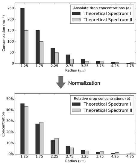
Figure 1.
Theoretical drop spectra: (a) absolute drop spectra; (b) relative drop spectra after normalization.
To investigate the different behavior of DSD in the three fog life cycle stages, the spectra were plotted for a first visual analysis. This made it possible to identify trends as well as unusual behavior in the data. After preprocessing and visual analysis, the data were split into the different fog life cycle stages, and for every stage, an average spectrum was derived. The representativity of the average spectra was calculated by means of Equation (A2). By using this formula, it was possible to make a statement of the explanatory power of the average spectrum of each stage.
The modified gamma distribution (MGD, Equation (A5)) was fitted to each 1-min spectrum using a least squares method implemented by Garbow et al. [36] following the Levenberg–Marquardt algorithm [37] to derive the parameters a, α, b, and γ. The fits were tested against the original DSD recordings using the Kolmogorov–Smirnov test as described in Adirosi et al. [38] to get an overview of the fitting performance. The MGD parameters were then analyzed to determine if the MGD parameters behaved differently in each stage of the fog life cycle. The proportionality factor Ω was derived for each single spectrum and each stage-averaged spectrum based on the MGD parameters using Equation (A18). In addition, the relationship between spectra-derived Z and LWC values was analyzed (Equations (A14) and (A17)). To investigate if it is possible to derive reliable Z-LWC relationships by means of the assigned characteristic DSD, sensitivity checks were done for the calculated values: First, Z values were derived using minimal and maximal LWC and values of the average spectra of each stage. Second, LWC values were calculated from minimal/maximal Z values and average spectra Ω values. In this way, it was possible to obtain information about the sensitivity of the Z-LWC relationship based on minimal/maximal LWC and Z values. In the last step, distributions were statistically tested for stage-dependent differences using the Kruskal–Wallis one-way analysis of variance by ranks [39] and three post hoc Mann–Whitney U-tests [31].
3. Results
The following section presents findings in regards to the temporal variability of DSD and its influence on the Z-LWC relationship. First, the different fog life cycle stages are checked for significantly different DSD characteristics. Next, we investigate if characteristic DSDs can be identified for the life cycle stages. Finally, we examine the possibility of deriving reliable Z-LWC relationships by means of a characteristic DSD.
3.1. Visual Analysis of DSD Differences for Different Fog Life Cycle Stages
Figure 2 shows the most important parameters measured during Fog Event 1, recorded between 26 October 2011 19:21 UTC and 27 October 2011 08:05 UTC. Subplot a shows absolute drop concentrations (number of drops per cm3 air volume per 0.5 μm radius interval). Subplot b shows relative drop concentrations (percentage of drops per 0.5 μm radius interval). The ordinate in Subplots a and b, representing the drop radii, only reaches 10 μm because the vast majority of drops had a measured radius between 1 μm and 10 μm. Intervals in which the drop concentration is higher are marked red, whereas intervals with low drop counts are colored white.
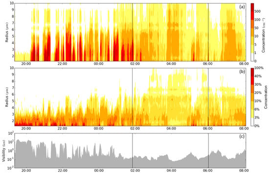
Figure 2.
Temporal evolution of the collected data during Fog Event 1: (a) absolute drop counts (b) relative drop counts (c) visibility. Vertical lines mark stage transitions.
During the formation stage, the largest average drop counts of up to were measured, while the mode radius largely remained below 3 μm. However, drop counts showed great temporal variability, as can be seen when looking at the vertical stripe pattern of the absolute drop spectra in this stage. During the mature stage, drop counts decreased to an average of , and the temporal variation in the drop spectra decreased compared to the formation stage. In this stage, mode radii were slightly larger than during fog formation, and a second, smaller local maximum appears at 7 μm in many spectra. This could possibly be the result of an instrument issue, as the maxima around 7 μm are very consistent over all measurements. As these maxima are comparatively small and the MGD has a unimodal shape with maxima usually found around 2 μm to 3 μm, these maxima are flattened out in the fitting procedure of the MGD and thus do not significantly interfere with the results.
Drop counts, mode radii and temporal variation during fog dissipation remained comparable to the values of the mature stage. During fog formation, horizontal visibility was highly variable between and with a general downward trend that reached close to zero by the end of the first stage. Visibility maintained approximately the same level in the mature stage, whereas during dissipation, it rose again, reaching 1.60 km at the end of the event.
Figure 3 shows the same information for Fog Event 2 recorded between 31 October 2011 17:38 UTC and 1 November 2011 07:55 UTC. This formation stage was also characterized by relatively large drop counts and small mode radii, which never exceeded 3 μm. During the first third of mature fog, large drop counts and small mode radii persisted; in the second third, the drop counts were significantly lower while mode radii rose to 6.75 μm. Towards the end of the mature stage and in the beginning of dissipation, drop counts increased again, while mode radii decreased to values below 2.5 μm. Subplot b reveals a local maximum at 7 μm, similar to the mature stage during the first fog event. After the last drop count maximum in the beginning of the dissipation period, values remained very low and never exceeded . Visibility values varied between 3.08 km and during formation, never exceeded 1.00 km during mature fog and, after some hesitation, rose to values between 2.00 km and 4.00 km during dissipation. At the very end of the fog event, it decreased again to .
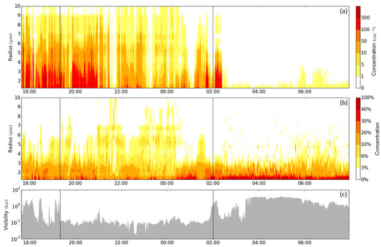
Figure 3.
Temporal evolution of the collected data during Fog Event 2: (a) absolute drop counts (b) relative drop counts (c) visibility. Vertical lines mark stage transitions.
The collected data from Fog Event 3, recorded between 13 November 2011 18:48 UTC and 14 November 2011 08:15 UTC are depicted in Figure 4. The first two thirds of the formation stage were characterized by large drop counts in combination with small mode radii. After that, very few drops were measured over a long period until the beginning of the mature stage when drop radii and counts increased rapidly. Throughout the whole mature stage, drop size spectra with large mode radii up to 7 μm were recorded. This stage was marked by very little variation in both drop counts and mode radii. Besides an abrupt decline around 07:00 UTC, during dissipation, drop radii and counts remained on a relatively even level. Visibility values during fog formation varied between and 2.95 km with no obvious trend. At the beginning of the mature stage, values decreased very abruptly to below and remained at this level throughout the entire mature stage. During dissipation, visibility values climbed up to 1.98 km for a short time, fell below again and then slowly rose to reach values of about .
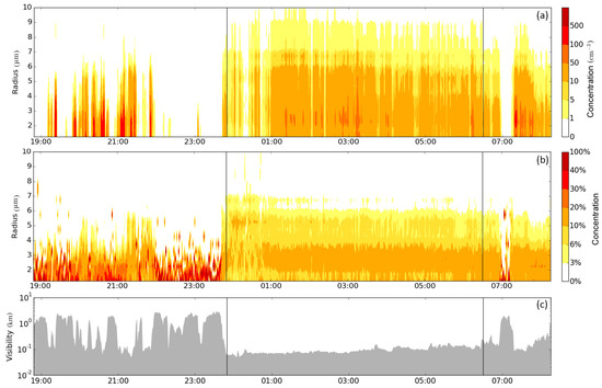
Figure 4.
Temporal evolution of the collected data during Fog Event 3: (a) absolute drop counts (b) relative drop counts (c) visibility. Vertical lines mark stage transitions.
In summary, maximal total drop counts appeared during the formation stage of each fog event investigated. The maximal values then continuously decreased through the mature and into the dissipation stages. The same pattern can be seen in the behavior of the mode radius drop counts (). The highest maximal values of were recorded during formation and continuously decreased until dissipation. During all three events, mode radii reached the highest recorded values during mature fog and the lowest values during dissipation. Maximal visibility values were observed in the formation stage of each event, but never exceeded 1.00 km during mature fog. During dissipation, a general uptick in visibility, albeit with high variability, could be detected. A brief overview of the information gathered during the three fog events is presented in Tables S1 and S2 (Supplementary Material), which summarize minimal and maximal values of the most important variables recorded.
3.2. Representativity of Average DSDs for Different Fog Life Cycle Stages
Average spectra were derived separately for each stage of each recorded fog event, as well as for the three combined life cycle stages of all fog events. In addition to the average spectra of the absolute values, the equivalent spectra of the relative values were calculated. Figure 5 and Figure 6 depict the absolute and relative average spectra separately for each stage. Although drop radii ranging from 1 μm to 25 μm were measured, only the first 19 intervals are shown as very few drops above 10 μm were recorded. The bar plots show the formation, mature fog and dissipation stage. Bars indicate stage-averaged values, while error bars denote the standard deviation. Note that the y-axis scale of Figure 5 is not uniform: absolute drop count averages were generally highest in the formation and lowest in the dissipation stage. All spectra show a slight bimodal structure with local maxima at 1.25 μm and 2.25 μm, although the second maximum is less pronounced than the first one. After the second maximum, the count generally decreases as the radius increases. The standard deviation is highest for small drop radii, where average count values are also highest. During Fog Event 1, most drops were recorded between 1.25 μm and 2.25 μm with a steep decline towards higher radii in the formation stage. In mature fog and during the dissipation stage, small droplets are less present, and the curve takes a more balanced shape. The spectra from the second fog event showed a similar behavior during formation, remained on a relatively high level for small radii in the mature stage, but then rapidly fell to smaller values, although drops with small radii between 1.25 μm and 2.75 μm were generally most frequent. The third fog event showed very similar average spectra in all stages, although drop counts were relatively small as compared to the other two fog events. Here too, small drop radii were best represented. However, during mature fog, the absolute maximum lay at 2.25 μm and drops with higher radii were significantly more common during this stage.
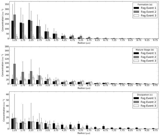
Figure 5.
Absolute average spectra in (a) Formation, (b) Mature Stage and (c) Dissipation.
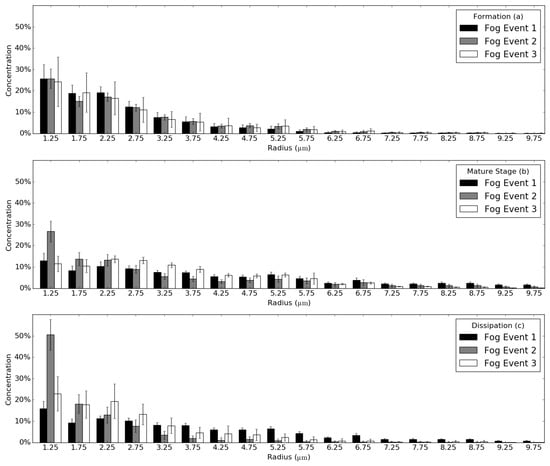
Figure 6.
Relative average spectra in (a) Formation, (b) Mature Stage and (c) Dissipation.
Figure 7 presents absolute and relative average spectra aggregated across all of the fog events in the study. Here, average spectra of all three fog life cycle stages are plotted on one chart. In most cases, absolute drop count averages reached their highest values in the formation stage and lowest in the dissipation stage. Here, considerable variation among small drop radii, the most commonly-occurring drop size, was recorded. All stages showed the previously-mentioned bimodal structure. During the formation stage, average drop counts were higher between radii of 1.25 μm and 2.25 μm although the difference from the other stages became less noticeable with increasing radii. The mature stage was characterized by lower drop counts for smaller radii and relatively high counts for larger radii, surpassing values of the formation stage from 5.25 μm upwards. This gives the average spectrum of the mature stage a more balanced form. Average drop counts during dissipation were generally very small compared to the other stages, and the absolute values showed a flat decline.
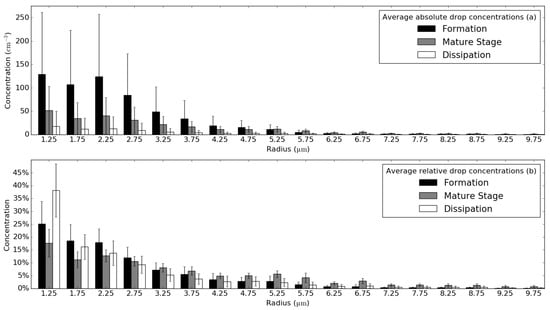
Figure 7.
Average spectra (over all three fog events): (a) Absolute drop concentrations and (b) relative drop concentrations.
Noteworthy is that the values of the relative average spectra were highest during dissipation, which steadily declined as radii increased. Here, the formation and dissipation stage spectra were unimodal (maximum at 1.25 μm). Only the mature stage spectrum continued to show the previously-mentioned bimodal structure, and the relative drop counts were comparably low at smaller radii and high at larger radii, exceeding the values of formation and dissipation at 3.25 μm and upwards. The representativity index of Equation (A2) was used to evaluate the explanatory power of the stage-averaged spectra. Table 2 depicts the results: the values represent the mean deviation of all spectra of one stage from the average spectrum of the respective stage, e.g., in the formation stage of Fog Event 1, the recorded spectra deviated from the mean spectrum by (absolute value) and by 46% (relative value). The absolute spectra always showed highest deviations during the formation and the lowest in the dissipation stage. Overall, formation deviated most from the mean during Fog Event 1 with , while Fog Event 2 showed the highest deviations in the mature and dissipation stages ( and , respectively). For all three stages, Fog Event 3 displayed the smallest values for stage-internal deviations from the absolute spectra. Deviations from the relative spectra are marked by different characteristics. Here, maximal deviations were observed during formation and dissipation in Fog Event 3 (79% and 65%, respectively). Compared to Fog Event 3 (19%), the mature stage showed higher values in Fog Events 1 (34%) and 2 (43%). Within the relative spectra, there was no identifiable general trend in the fog life cycle stages. Although Fog Event 1 still reflected the pattern: formation > mature fog > dissipation, this was reversed in Fog Event 2, where the highest deviation values were reached in dissipation (43%) and the lowest values in formation (30%). Fog Event 3 showed yet another behavior with minimal values during mature fog (19%) and far higher values in formation and dissipation (79% and 65%, respectively). The last line in Table 2 lists deviation values of all spectra of one stage from the respective average spectrum aggregated across all investigated fog events (cf. Figure 7). Similar to the absolute data of the single fog events, the overall deviations were highest for the formation stage () and lowest for the dissipation stage (). The relative spectra showed the highest deviations for the dissipation stage (60%) and the lowest for mature fog (41%).
Table 2.
Representativity R (cm−3) of the average spectra.
3.3. The Z-LWC Relationship
3.3.1. Derived Parameters of the Modified Gamma Distribution
Parameters of the modified gamma distribution (MGD) were derived for each minute-averaged spectrum, as well as for the three stage-averaged spectra. The MGD parameters of the stage-averaged spectra and the respective graphs of the functions over all fog events are presented in Table 3 and Figure 8. values were similar in formation and mature fog, but differed considerably from the dissipation stage (0.50 μm). The Kolmogorov–Smirnov test was applied to each measured 1 min spectrum and its corresponding MGD fit. The acceptance rate at the significance level was 87.1%, 91.8% and 97.8% for formation, mature stage and dissipation. The good performance of the fits can partly be attributed to the fact that many DSDs showed small total droplet numbers , which naturally results in larger p values.
Table 3.
MGD parameters of stage-averaged spectra.
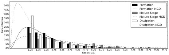
Figure 8.
Fitted MGDs to stage-averaged spectra over all three fog events.
3.3.2. The Proportionality Factor Ω
As a last step, Ω values were derived from each MGD parameter set presented in the previous section. Large Ω values mean that LWG values are large in comparison to the corresponding Z values (cf. Equation (A18)). This ratio arises, when the DSD is strongly right-skewed, meaning there are many small droplets and very few large droplets. On the other hand, small Ω values mean that LWG values are small in comparison to the corresponding Z values, which is the result of a more balanced DSD with fewer small droplets and more large droplets.
Table 4 gives an overview of the most important descriptive measures of Ω in the different fog events (Nos. 1, 2 and 3) and life cycle stages: formation (F), mature stage (M) and dissipation (D). The smallest range, standard deviation and maximum values of Ω were detected in the dissipation stage of Fog Event 1, whereas the largest range and largest maximum values were found in the formation stage of Fog Event 2. Combined over all investigated fog events, the formation stage showed the highest range and the highest maximum with . The mature stage showed minimal values in range and standard deviation with and , respectively. However, these trends are not evident when the single fog events are viewed separately. While the range and standard deviation values decreased throughout the life cycle of Fog Event 1, Fog Event 2 showed the opposite behavior with minimal values in formation and maximum values in dissipation.
Table 4.
Statistical measures of Ω derived from the MGD parameters of the three fog events. Formation (F), mature stage (M) and dissipation (D): Minimum (Min.), Mean, Maximum (Max.), Range, Standard Deviation (STD), 5% Percentile (5% PCTL) and 95% Percentile (95% PCTL).
Figure 9 provides an overview of the MGD parameters , and while considering the Z-LWC relationship factor Ω. Each parameter set is colored according to its corresponding Ω value. Ninety percent of the values lay between and . Minimal Ω values were only found where all parameters simultaneously had small values. A strip cluster of “blue” sets along the -axis indicates Ω values that lie below .
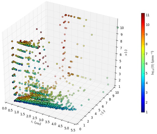
Figure 9.
MGD parameter sets of Fog Events 1, 2 and 3 colored after Ω.
Figure 10 shows the general tendencies of the different Ω distributions. Median Ω values of in formation, in mature fog and in dissipation indicate differences between all three stages.
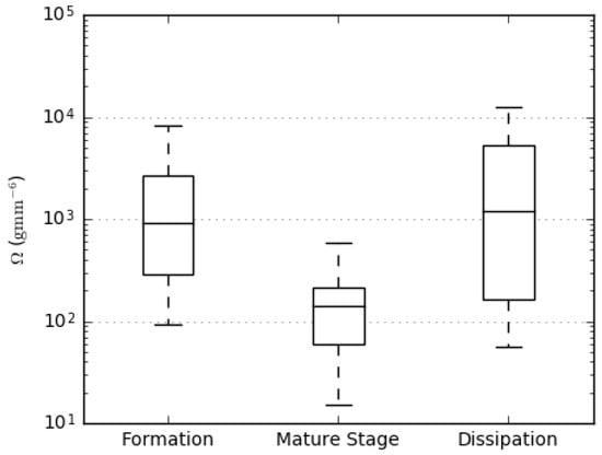
Figure 10.
General tendencies of Ω distributions.
To test for statistically-significant differences between the three distributions, the non-parametric Kruskal–Wallis one-way analysis of variance by ranks [39] was conducted, as the data were not normally distributed. Outliers of more than three standard deviations were excluded. Of the 98.77% of the data included, the test reported a statistically-significant difference between the fog life cycle stages (). In order to determine between which of the three fog life cycle stages these statistically-significant differences can be found, three post hoc Mann–Whitney U-tests [31] were conducted. The Bonferroni method was used to correct the level of significance, which yielded a total of . The results showed a significant difference between formation and mature fog (), as well as between mature fog and dissipation (). However, no significant difference at the corrected significance level was found between the formation and dissipation distributions ().
3.3.3. Derivation of Reliable Z-LWC Relationships by Means of Stage-Dependent Characteristic DSDs
The scatterplots depicted in Figure 11 show the relationship between Z and LWC for each fog life cycle stage. Both Z and LWC were derived from the MGD parameters using Equations (A14) and (A17) in the Appendix A. The formation stage showed a wide range of Z values with 5% and 95% percentiles at −46.1 dBZ and −28.4 dBZ. No unique LWC value could be assigned to one specific Z value between −45.0 dBZ and −30.0 dBZ, as a vast dispersion of LWC values ranging between and occurred. For Z below −60.0 dBZ, the corresponding LWC diminished to marginally small values (Figure 11a). During mature fog, the range of Z values narrowed considerably, with 90% of the data between −32.7 dBZ and −22.0 dBZ. Nonetheless, the values were generally higher with a mean of −34.3 dBZ compared to −54.1 dBZ in the formation stage. In the mature stage, unique LWC values could be assigned to the respective Z values more precisely, as the dispersion of LWC values was smaller in this stage for constant Z values (Figure 11b). During the dissipation stage, the range on the Z-axis rose again with 90% of the values between −68.7 dBZ and −27.5 dBZ. The spread of LWC values decreased to a range of . Due to the narrow range of LWC values for constant Z values, Z values were most accurately assigned to the respective LWC values in the dissipation stage.
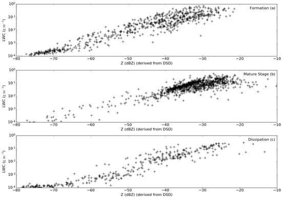
Figure 11.
Derived LWC vs. derived Z for all three fog events in (a) Formation, (b) Mature stage and (c) Dissipation.
The results of the sensitivity tests are listed in Table 5. The Z values represent values derived from 5% and 95% confidence intervals, as well as median LWC values and the corresponding average spectrum Ω. The minimum of −74.9 dBZ was reached for the formation average spectrum, whereas the maximum was recorded in the mature stage with −25.2 dBZ. LWC values were derived from 5% and 95% confidence intervals, as well as median Z values of the corresponding stage in combination with its average spectrum Ω. The maximum () was found in the mature stage, whereas the minimum () was found in the dissipation stage.
Table 5.
Derived Z and LWC values of the sensitivity tests.
4. Discussion
This study seeks to answer the following questions: (i) Do fog life cycle stage-dependent differences exist in the DSD? (ii) Can characteristic DSDs be identified for each stage? (iii) How reliable are the LWC values derived from radar reflectivity Z, using the relationship factor as defined above? These questions are discussed in the following paragraphs.
4.1. Differences in DSDs between Fog Life Cycle Stages
Fog Events 1, 2 and 3 showed DSDs that are characteristic of radiative fog events: The vast majority of the measured drops lay below 10 μm radius with mode radii largely below 3 μm. Furthermore, total drop counts never exceeded (cf. Table S2 Supplementary Material). These values are consistent with data recorded by Harris [40], who reported values between 2 μm and 4 μm radius for radiation fogs, as well as the data presented in Arnulf et al. [41], Best [42], Eldridge [43] and Garland [44] with values reaching up to for radiation fogs.
The first indication of stage-dependent DSD differences can be found in Figure 2, Figure 3 and Figure 4, which are supported by Table S2 (Supplementary Material). Formation stages were characterized by large temporal variations in the DSD, relatively small values and high that steeply declined as drop radius increased. Compared to this, mature stages showed less temporal variation, fewer, but in general larger drops and a more balanced DSD with equal counts in many radius intervals. During dissipation, , as well as values decreased to the lowest level in all three investigated fog events, while the temporal variations in DSD increased again. Stage-dependent differences in DSD were also present in the average spectra over each stage (Figure 7). Absolute drop counts clearly show that the highest values were reached for all size bins up to 4.75 μm during formation and rapidly declined towards bigger radii. In mature fog, absolute drop counts were significantly lower for small radii, but values exceeded those of the formation stage at radii above 4.75 μm due to a relatively flat decline. The lowest absolute values were recorded for all size bins during dissipation. Relative drop counts show that formation and dissipation were characterized by a similar kurtosis. Here, the mature stage differed with smaller relative values in small-sized bins and larger relative values in large-sized bins. In addition to these differences, there were also differences within each stage: besides the different stage durations, a major discrepancy within the stages was apparent in values, which reached a maximum of in the formation of Fog Event 1 as opposed to a maximum of in the formation of Fog Event 3. Additionally, the mature stage of Fog Event 3 displayed different behavior from the other two mature stages with extremely constant spectra throughout the whole stage compared to the fluctuating spectra of Fog Events 1 and 2. An exception in the dissipation stage can be identified in Fog Event 2. Here, the decline towards larger radii was more pronounced than in the other fog events, where drops above 5 μm had similar frequencies to the smaller drops. Thus, we conclude there are stage-dependent differences in DSD, but it is not possible to derive general stage characteristics applicable to all three fog events. Each stage has unique properties specific to the respective fog event. Parameters of the derived MGD were also analyzed for stage-dependent differences (cf. Figures S1–S3 in the Supplementary Materials). These results led to similar conclusions. In all three fog events, each stage showed its own characteristics with formation parameter sets generally showing the largest variability on all axes. The parameters of the dissipation stage showed similar behavior albeit with less variability, whereas the mature stage parameters were closely bulked on the - and -axes. However, again, no general statement can be made of the stages aggregated across all fogs.
Ω values are indicators of the shape of the MGD and therefore describe the relationship between Z and LWC. Hence, we tested how Ω values were distributed depending on the fog life cycle stage (cf. Figure 10). The boxplots show that formation and dissipation consisted of DSDs with a wide spectrum of Ω values; the 5% and 95% confidence levels fell at and , respectively. This indicates large variations in the steepness and maxima of the DSD curves. On the other hand, the mature stage showed Ω values that rarely exceeded (5% and 95% confidence interval), which indicates that most DSDs were characterized by large mode radii and a flat overall curve during this stage. The range of Ω values, which declined from formation ( to ) through mature fog ( to ) to dissipation ( to ), is comparable to the results of Maier et al. [4].
However, the conclusion that Ω values generally decreased over time and that the curves steepened with decreasing mode radii, respectively, cannot be made, as the fact that the mature stage DSDs showed generally much smaller Ω values with less variation is much more important than the mode alone. Results of the statistical analysis confirm a difference between the mature stage and both other stages. However, the results of the Mann–Whitney U-test for differences between formation and dissipation did not result in a significant output. Therefore, it cannot be affirmed that there is a difference between the DSDs of the formation and the dissipation stage, at least not for the investigated fog events. To summarize, the results concerning the first question, fog life cycle stage-dependent differences in the DSD can only be individually affirmed for each fog event, but not for all fogs in total. The derivation of microphysical conditions that are characteristic for a certain stage is not applicable to more than a single fog event.
4.2. Representativity of Stage-Averaged Spectra
The second question addressed the assumption that the different fog life cycle stages could be represented by characteristic DSDs. In other words, we assumed that the intra-stage variation was low enough to be able to make a general and valid statement about the behavior of the respective mean DSD as representative for the whole stage. To test this assumption, average spectra and the representativity index (Equation (A2)) were calculated for the formation, mature and dissipation stages, respectively. Average spectra are depicted in Figure 5, Figure 6 and Figure 7, and the representativity indices are listed in Table 2. Figure 7 indicates that variability was very high compared to the respective average values during all stages. For radii below 4.75 μm in particular, extremely high values were calculated for the standard deviation with values of more than two-times the mean value. This provides an initial overview of the magnitude of variability in the data.
Similar to the average drop count differences between single fog events, however, the variability in the data changed from one fog event to the next. This complicates the ascertainment of variability values for all fog events studied. Figure 5 shows that the variability during the formation stage of Fog Event 3 with a maximal standard deviation of within one radius interval was much smaller than those of Fog Events 1 and 2 ( and ). During the mature stage, Fog Event 2 showed much higher standard deviations than Fog Events 1 and 3, while the variability in each fog event was approximately equal in the dissipation stage. The representativity indices in Table 2 lead to the same conclusions. Collectively across all fog events, the formation stage suffered from the largest absolute representativity values with an average deviation of from the average spectrum. Mature fog () and dissipation () had much smaller values, and consequently, their absolute average spectra represented their respective stage considerably better than the average spectrum of the formation stage. However, the representativity values themselves showed significant differences between the three fog events. For instance, only Fog Events 1 and 2 showed high absolute representativity values during formation ( and ), whereas Fog Event 3 showed far less variability with an R of . Variability in the mature stage was nearly four-times higher in Fog Event 2 than in both other fog events. Only the dissipation stage showed similar values across all three fog events. Thus, we again conclude it is not possible to make general statements about the fog life cycle stages. Each fog event shows its own stage characteristics.
The R values of the relative spectra reveal yet another peculiarity. Here, the lowest values were recorded during mature fog (0.41) and the highest during dissipation (0.60). This means that the drops measured during the dissipation stage were, on average, distributed differently by 60% over the 48 size bins. During formation 57% and during mature fog 41% were calculated as an average value, respectively. This in turn means that not only the absolute drop counts varied between spectra, but that the shape of the spectrum itself was subject to high variability, leading to steep curves with small mode radii, on the one hand, as well as flat curves with large mode radii, on the other hand. While the R value of the absolute spectra of the formation stage was smallest in Fog Event 3 (), the same stage of the same fog event had the highest respective R value of the relative spectra (0.79). The small absolute value was the result of a generally low total drop count during the formation of Fog Event 3. However, skewness and kurtosis of the curves differed strongly during this stage, which is reflected in the high R value of the relative spectra. Again, each fog event is marked by unique characteristics, so a general conclusion from the aggregated values of all fogs has to be treated carefully. Figures S1–S3 in the Supplementary Materials graphically support these conclusions. Here, the high variability in the shape of the curves during fog formation and dissipation are represented in the different values that the MGD parameters take. The mature stage showed less variability in its parameter sets, which correlates well with the R values of the relative spectra in Table 2. The high standard deviation and representativity values indicate that it is difficult to determine the general characteristics of an entire fog life cycle stage from only one average spectrum. Thus, it is only possible to identify characteristic DSDs for the absolute drop counts of the dissipation stage, where the representativity values were much smaller than in both other stages. However, looking at the relative drop counts, a general statement about the curve’s kurtosis and skewness is not possible with only one average spectrum as there is too much variability in the data, especially in the dissipation stage.
4.3. Feasibility of the Z-LWC Approach
The third question addresses the reliability of the LWC values derived from radar reflectivity Z, using the relationship factor Ω as defined above. Hence, we investigated whether it is possible to derive characteristic stage-averaged DSDs and their respective Ω values. The MGD parameters of the defined stage-representing spectra are listed in Table 3, and the corresponding functions are depicted in discrete and continuous form in Figure 8. In a first step, Z and LWC values were derived from all DSD spectra that were recorded during the ground-based measurements of Fog Events 1, 2 and 3 using Equations (A14) and (A17). This was done to get an overview of the range of LWC values at known Z values during formation, mature fog and dissipation. The results of Figure 11 show that it should be possible to derive LWC values more precisely from measured Z values, especially during dissipation, as the spread on the y-axis is smallest in this stage. However, the LWC values themselves were very small in this stage with 95% remaining below , so deriving LWC values in relation to their absolute value was no more precise than in the other stages. The highest absolute spread of LWC values was identified for the formation stage. This shows that reliably deriving LWC values from recorded Z values at a known DSD should be very difficult in this stage.
As a second step, two sensitivity checks were conducted. They tested the range of Z and LWC values derived from each other’s extremes. The results in Table 5 show that the values of Z, derived from measured LWC values, lie in a reasonable range with a minimum of −74.9 dBZ and a maximum of −25.2 dBZ. The range of derived Z values using only one static Ω value in each stage strongly correlated with the Z range when Ω values that were derived individually for each spectrum were used. The decrease in the range over the fog life cycle and the simultaneous shift towards higher Z values can be attributed to the small Ω value that was used for the dissipation stage () compared to and for formation and mature stage. The LWC values derived from typical Z values for each stage showed realistic ranges in the formation stage with a maximum of . For the mature and dissipation stages the maxima of and also lay within the typical values during radiation fog events, which can reach up to [45,46].
5. Conclusions
This study investigated the temporal variability of the DSD of fog and its influence on the Z-LWC relationship. In this context, microphysical data of three radiation fog events were analyzed for stage-dependent differences. In addition, fog life cycle stages were tested to determine whether they show typical DSD characteristics, which could be used to separately infer a static relationship between Z and LWC for each stage. As a last step, this information was used to test the feasibility of deriving LWC values directly from radar reflectivity measurements by means of the established relationship factor Ω.
Reliable Z-LWC relationships would enable the retrieval of LWC profiles from cloud radar reflectivity with high temporal and vertical resolution. Besides a better understanding of the microphysical processes involved in fog formation and dissipation, satellite-based fog detection techniques, e.g., Cermak and Bendix [10], could be improved if reliable LWC profiles were available for initialization and validation. Straightforward fog models, e.g., Reudenbach and Bendix [47], that rely on columnar LWC data would be able to provide better results if precise LWC input data from radar-based retrievals were available. Finally, these improvements could lead to more precise fog detection and forecasting results.
The results showed that the average DSD of each stage differed from those of the other stages in mode radius, kurtosis and skewness. However, general DSD characteristics for the stages could not be derived because of their inherent heterogenic structure. The variability within each stage combined with the fact that each stage showed different properties dependent on the particular fog event prevented the identification of one specific fog-independent relationship factor for the life cycle stages. To gain more significant results, more continuous DSD measurements during different radiation fog events on the ground, as well as vertical profiles are needed.
Concerning the applied MGD, it has to be mentioned that every fitting approach has its intrinsic limits and errors, which affect the output results. Following former studies related to fog DSD, the MGD is appropriate for reliably representing the various DSDs during the respective development stages of radiation fog events, e.g., Tampieri and Tomasi [48], Tomasi and Tampieri [49] and Maier et al. [4]. However, studies related to DSD of raindrops indicated that even the three-parameter MGD shows limitations comparing the modeled to the measured DSDs, e.g., Joss and Gori [50], Ulbrich [51] and Adirosi et al. [38]. To some extent these limitations can also be stated for the derived MGD parameters in this study. For example, due to the lack of information about droplet counts in the radius range between 0 μm and 1 μm, the derived MGD parameters might be imprecise. With respect to the relationship between Z and LWC, it would be possible to retrieve both parameters from the measured DSDs and to use a nonlinear regression to obtain coefficients relating LWC to Z, instead of using the proportionality factor Ω. One disadvantage in the mentioned approach, however, would be the complete omission of the small droplet sizes below 1 μm radius, which might also lead to inaccuracies in the retrieved Z-LWC relationship. Furthermore, it would be difficult to relate the differing Z-LWC relationship directly to the high temporal DSD dynamics during fog development. By using the derived MGD parameters, the comparison with other studies, e.g., Harris [40], Tampieri and Tomasi [48], Tomasi and Tampieri [49], Maier et al. [4] and Maier et al. [30] is facilitated. Nevertheless, the difference between both procedures should be investigated in future studies, using more continuous DSD measurements during different radiation fog events.
The DSD measurements for the fog events observed will be made freely available for download at www.lcrs.de (data).
Supplementary Materials
The following are available online at www.mdpi.com/2073-4433/8/8/142/s1: Table S1: Minima of meteorological and microphysical variables; Table S2: Maxima of meteorological and microphysical variables; Figure S1: MGD parameters of Fog Event 1; Figure S2: MGD parameters of Fog Event 2; Figure S3: MGD parameters of Fog Event 3.
Acknowledgments
The authors would like to thank the German Research Foundation (DFG) for funding the project (TH1531/1-1). The authors are also thankful to Sebastian Achilles for his support during the measurements.
Author Contributions
Boris Thies and Jörg Bendix conceived of and designed the experiments. Boris Thies and Sebastian Egli performed the experiments. Sebastian Egli analyzed the data. Boris Thies and Sebastian Egli contributed analysis tools and materials. Boris Thies and Sebastian Egli wrote the paper.
Conflicts of Interest
The authors declare no conflict of interest. The founding sponsors had no role in the design of the study; in the collection, analyses or interpretation of data; in the writing of the manuscript; nor in the decision to publish the results.
Abbreviations
The following abbreviations are used in this manuscript:
| BM | Weather classification: zonal ridge across Central Europe |
| CDP | Cloud Droplet Probe |
| DSD | Drop size distribution |
| FMCW | Frequency-modulated continuous wave technique |
| HNA | Weather classification: high pressure ridge over Central Europe |
| LWC | Liquid water content |
| MGD | Modified gamma distribution |
| SA | Weather classification: anticyclonic southerly |
| SEZ | Weather classification: cyclonic south-easterly |
| Z | Radar reflectivity |
Appendix A
In discrete form, the DSD can be defined as:
where is the total number of drops per unit volume of air. m is the number of channels used and is the droplet number concentration of each channel. Using the following formula, the representativity of a mean spectrum in relation to its fog life cycle stage can be assessed:
R is the representativity of the stage’s average spectrum. It is defined as the average of the summed absolute differences between all radius interval drop counts of all measured spectra of one life cycle stage and its average spectrum. n is the number of spectra of one stage; m is the number of intervals per spectrum, in this case 48; is the j-th interval value of spectrum i; and is the j-th interval value of the average spectrum.
In continuous form the DSD in fog can be represented by a function of the form:
where is the total concentration per unit volume of air of particles with radii between and [52]. is a spectral density function, which will give the total number of particles in a given radius interval when integrated with respect to r. It can be written as:
with being the total number of particles within the given volume of air and being a suitable normalized probability density function (PDF). In the context of fog and cloud droplet analysis, many size distributions have been proposed, e.g., normal, logarithmic normal or gamma distributions. The most commonly-used PDF is the modified gamma distribution (MGD), which, itself, comes in many variations, each one adequate for a different problem. In this study, the version proposed by Deirmendjian [53] is used:
The three parameters a, b and are positive real numbers, whereas is a positive integer. a is called the normalization factor, as it is only related to , and it ensures that the integral of the MGD over all radii is equal to . The shape of the MGD is determined by b and , which can be called the slope and shape parameter, respectively. The MGD has two zeros, one at and one at . Its first derivative:
has three zeros, the first at and the second at . The third zero can be found by putting the last factor in Equation (A6) to zero, which yields the absolute maximum of the MGD and, thus, gives the mode radius [53]:
According to Gradshteyn and Ryzhik [54], the moments of the MGD can be written as:
which provides the integral:
with the gamma function:
The radar reflectivity factor Z can be simply formulated as:
Its unit can be stated as or as a logarithmic measure according to:
with [55,56].
Merging the DSD from Equation (A5) with Equation (A11) results in:
which, after integrating over the range of radii (see Equation (A9)), yields in [4]:
Equation (A14) provides a direct connection between radar reflectivity Z and the drop size spectrum, expressed in terms of the modified gamma distribution. The LWC can be expressed with the usage of the DSD as it is only dependent on the drop size spectrum and the absolute mass of drops in the given volume of air. Assuming only spherical water particles in the studied fog events, one can define:
with:
where is the water density of 1 g cm−3 [4]. Inserting Equation (A3) into Equation (A13) results after integration over all radii in:
The Z-LWC relationship can be derived by dividing Equation (A17) by Equation (A14), which provides the proportionality factor , thus giving a direct relationship between Z and LWC [4]:
Now that we have established a connection between Z and LWC using the information provided by the DSD, we can deduce LWC values from given Z values by means of Equation (A18).
References
- Nemery, B.; Hoet, P.H.M.; Nemmar, A. The Meuse Valley fog of 1930: An air pollution disaster. Lancet 2001, 357, 704–708. [Google Scholar] [CrossRef]
- Pinto, R.; Larrain, H.; Cereceda, P.; Lázaro, P.; Osses, P.; Schemenauer, R.S. Monitoring fog-vegetation communities at a fog-site in Alto Patache, South of Iquique, Northern Chile, during “El Niño” and “La Niña” events (1997–2000). In Proceedings of the Second International Conference on Fog and Fog Collection, International Development Research Center, Ottawa, ON, Canada, 15–20 July 2001; pp. 293–296. [Google Scholar]
- Sampurno Bruijnzeel, L.; Eugster, W.; Burkard, R. Fog as a Hydrologic Input. In Encyclopedia of Hydrological Sciences; John Wiley & Sons, Ltd.: Chichester, UK, 2005; pp. 559–582. [Google Scholar]
- Maier, F.; Bendix, J.; Thies, B. Simulating Z-LWC relations in natural fogs with radiative transfer calculations for future application to a cloud radar profiler. Pure Appl. Geophys. 2012, 169, 793–807. [Google Scholar] [CrossRef]
- Schulze-Neuhoff, H. Nebelfeinanalyse mittels zusätzlicher 420 Klimastationen—Taktische Analyse 1:2 statt 1:5 Mill. Meteorol. Rundsch. 1976, 29, 75–84. [Google Scholar]
- Gultepe, I.; Tardif, R.; Michaelides, S.C.; Cermak, J.; Bott, A.; Bendix, J.; Müller, M.D.; Pagowski, M.; Hansen, B.; Ellrod, G.; et al. Fog Research: A Review of Past Achievements and Future Perspectives. Pure Appl. Geophys. 2007, 164, 1121–1159. [Google Scholar] [CrossRef]
- Terradellas, E.; Bergot, T. Comparison between two-single-column models designed for short-terms fog and low-clouds forecasting. Física de la Tierra 2007, 19, 189–203. [Google Scholar]
- Cermak, J.; Bendix, J. A novel approach to fog/low stratus detection using Meteosat 8 data. Atmos. Res. 2008, 87, 279–292. [Google Scholar] [CrossRef]
- Bendix, J.; Thies, B.; Cermak, J.; Nauß, T. Ground Fog Detection from Space Based on MODIS Daytime Data—A Feasibility Study. Weather Forecast. 2005, 20, 989–1005. [Google Scholar] [CrossRef]
- Cermak, J.; Bendix, J. Detecting ground fog from space—A microphysics-based approach. Int. J. Remote Sens. 2011, 32, 3345–3371. [Google Scholar] [CrossRef]
- Kollias, P.; Clothiaux, E.E.; Miller, M.A.; Albrecht, B.A.; Stephens, G.L.; Ackerman, T.P. Millimeter-wavelength radars: New frontier in atmospheric cloud and precipitation research. Bull. Am. Meteorol. Soc. 2007, 88, 1608–1624. [Google Scholar] [CrossRef]
- Nowak, D.; Ruffieux, D.; Agnew, J.L.; Vuilleumier, L. Detection of fog and low cloud boundaries with ground-based remote sensing systems. J. Atmos. Ocean. Technol. 2008, 25, 1357–1368. [Google Scholar] [CrossRef]
- Sauvageot, H.; Omar, J. Radar Reflectivity of Cumulus Clouds. J. Atmos. Ocean. Technol. 1987, 4, 264–272. [Google Scholar] [CrossRef]
- Liao, L.; Sassen, K. Investigation of relationships between Ka-band radar reflectivity and ice and liquid water contents. Atmos. Res. 1994, 34, 231–248. [Google Scholar] [CrossRef]
- Sassen, K.; Liao, L. Estimation of Cloud Content by W-Band Radar. J. Appl. Meteorol. 1996, 35, 932–938. [Google Scholar] [CrossRef]
- Fox, N.I.; Illingworth, A.J. The Retrieval of Stratocumulus Cloud Properties by Ground-Based Cloud Radar. J. Appl. Meteorol. 1997, 36, 485–492. [Google Scholar] [CrossRef]
- Donovan, D.P.; van Lammeren, A.C.A.P. Cloud effective particle size and water content profile retrievals using combined lidar and radar observations: 1. Theory and examples. J. Geophys. Res. 2001, 106, 27425. [Google Scholar] [CrossRef]
- Löhnert, U.; Crewel, S.; Simmer, C.; Macke, A. Profiling cloud liquid water by combining active and passive microwave measurements with cloud model statistics. J. Atmos. Ocean. Technol. 2001, 18, 1354–1366. [Google Scholar] [CrossRef]
- Frisch, A.S.; Fairall, C.W.; Snider, J.B. Measurement of Stratus Cloud and Drizzle Parameters in ASTEX with a Kα–Band Doppler Radar and a Microwave Radiometer. J. Atmos. Sci. 1995, 52, 2788–2799. [Google Scholar] [CrossRef]
- Khain, A.; Pinsky, M.; Magaritz, L.; Krasnov, O.; Russchenberg, H.W.J. Combined observational and model investigations of the Z-LWC relationship in stratocumulus clouds. J. Appl. Meteorol. Climatol. 2008, 47, 591–606. [Google Scholar] [CrossRef]
- Pilié, R.J.; Mack, E.J.; Kocmond, W.C.; Eadie, W.J.; Rogers, C.W. The Life Cycle of Valley Fog. Part II: Fog Microphysics. J. Appl. Meteorol. 1975, 14, 364–374. [Google Scholar] [CrossRef]
- Meyer, M.B.; Lala, G.G.; Jiusto, J.E. Fog-82: A Cooperative Field Study of Radiation Fog. Bull. Am. Meteorol. Soc. 1986, 67, 825–832. [Google Scholar] [CrossRef]
- Welch, R.M.; Ravichandran, M.G.; Cox, S.K. Prediction of Quasi-Periodic Oscillations in Radiation Fogs. Part I: Comparison of Simple Similarity Approaches. J. Atmos. Sci. 1986, 43, 633–651. [Google Scholar] [CrossRef]
- Wendisch, M.; Mertes, S.; Heintzenberg, J.; Wiedensohler, A.; Schell, D.; Wobrock, W.; Frank, G.; Martinsson, B.G.; Fuzzi, S.; Orsi, G.; et al. Drop size distribution and LWC in Po Valley fog. Contrib. Atmos. Phys. 1998, 71, 87–100. [Google Scholar]
- Guyot, G.; Gourbeyre, C.; Febvre, G.; Shcherbakov, V.; Burnet, F.; Dupont, J.C.; Sellegri, K.; Jourdan, O. Quantitative evaluation of seven optical sensors for cloud microphysical measurements at the Puy-de-Dôme Observatory, France. Atmos. Meas. Tech. 2015, 8, 4347–4367. [Google Scholar] [CrossRef]
- Egli, S.; Maier, F.; Bendix, J.; Thies, B. Vertical distribution of microphysical properties in radiation fogs—A case study. Atmos. Res. 2015, 151, 130–145. [Google Scholar] [CrossRef]
- Droplet Measurement Technologies (DMT). Data Analysis User’s Guide Chapter I : Single Particle Light Scattering; Droplet Measurement Technologies: Boulder, CO, USA, 2009; p. 44. [Google Scholar]
- Lance, S.; Brock, C.A.; Rogers, D.; Gordon, J.A. Water droplet calibration of the Cloud Droplet Probe (CDP) and in-flight performance in liquid, ice and mixed-phase clouds during ARCPAC. Atmos. Meas. Tech. 2010, 3, 1683–1706. [Google Scholar] [CrossRef]
- Bristol Industrial & Research Associates Ltd (Biral). HSS VPF-730 Combined Visibility & Present Weather Sensor; Bristol Industrial and Research Associates Limited: Portishead, Bristol, UK, 2012; p. 2. [Google Scholar]
- Maier, F.; Bendix, J.; Thies, B. Development and application of a method for the objective differentiation of fog life cycle phases. Tellus Ser. B 2013, 65, 1–17. [Google Scholar] [CrossRef]
- Mann, H.B.; Whitney, D.R. On a Test of Whether one of Two Random Variables is Stochastically Larger than the Other. Ann. Math. Stat. 1947, 18, 50–60. [Google Scholar] [CrossRef]
- Kendall, M. Rank Correlation Methods, 4th ed.; Hodder Arnold: London, UK, 1976; p. 210. [Google Scholar]
- Fisher, R. Statistical Methods for Research Workers, 5th ed.; Oliver & Boyd: Edinburgh, UK, 1925; p. 336. [Google Scholar]
- Hess, P.; Brezowsky, H. Katalog der Grosswetterlagen Europas 1881–1976, 3. verbesserte und ergänzte Aufl.; Deutscher Wetterdienst: Offenbach am Main, Germany, 1977; p. 68. [Google Scholar]
- James, P.M. An objective classification method for Hess and Brezowsky Grosswetterlagen over Europe. Theor. Appl. Climatol. 2007, 88, 17–42. [Google Scholar] [CrossRef]
- Garbow, B.S.; Hillstrom, K.E.; More, J.J. Documentation for MINPACK subroutine LMDIF; Argonne National Laboratory: Argonne, IL, USA, 1980. [Google Scholar]
- Marquardt, D.W. An Algorithm for Least-Squares Estimation of Nonlinear Parameters. J. Soc. Ind. Appl. Math. 1963, 11, 431–441. [Google Scholar] [CrossRef]
- Adirosi, E.; Volpi, E.; Lombardo, F.; Baldini, L. Raindrop size distribution: Fitting performance of common theoretical models. Adv. Water Resour. 2016, 96, 290–305. [Google Scholar] [CrossRef]
- Kruskal, W.H.; Wallis, W.A. Use of Ranks in One-Criterion Variance Analysis. J. Am. Stat. Assoc. 1952, 47, 583. [Google Scholar] [CrossRef]
- Harris, D. The attenuation of electromagnetic waves due to atmospheric fog. Int. J. Infrared Millim. Waves 1995, 16, 1091–1108. [Google Scholar] [CrossRef]
- Arnulf, A.; Bricard, J.; Curé, E.; Véret, C. Transmission by Haze and Fog in the Spectral Region 0.35 to 10 Microns. J. Opt. Soc. Am. 1957, 47, 491–497. [Google Scholar] [CrossRef]
- Best, A.C. Drop-size distribution in cloud and fog. Q. J. R. Meteorol. Soc. 1951, 77, 418–426. [Google Scholar] [CrossRef]
- Eldridge, R.G. Haze and Fog Aerosol Distributions. J. Atmos. Sci. 1966, 23, 605–613. [Google Scholar] [CrossRef]
- Garland, J.A. Some fog droplet size distributions obtained by an impaction method. Q. J. R. Meteorol. Soc. 1971, 97, 483–494. [Google Scholar] [CrossRef]
- Pilié, R.; Eddie, W.; Mack, E.; Rogers, C.; Kocmond, W. Project Fog Drops Part I: Investigations of Warm Fog Properties; Technical Report August; Cornell Aeronautical Laboratory, Inc.: Buffalo, NY, USA, 1972. [Google Scholar]
- Garland, J.A.; Branson, J.R.; Cox, L.C. A study of the contribution of pollution to visibility in a radiation fog. Atmos. Environ. 1973, 7, 1079–1092. [Google Scholar] [CrossRef]
- Reudenbach, C.; Bendix, J. Experiments with a straightforward model for the spatial forecast of fog/low stratus clearance based on multi-source data. Meteorol. Appl. 1998, 5, 205–216. [Google Scholar] [CrossRef]
- Tampieri, F.; Tomasi, C. Size distribution models of stratospheric particles in terms of the modified gamma function. Arch. Meteorol. Geophys. Bioklimatol. Ser. A 1976, 25, 47–54. [Google Scholar] [CrossRef]
- Tomasi, C.; Tampieri, F. Features of the proportionality coefficient in the relationship between visibility and liquid water content in haze and fog. Atmosphere 1976, 14, 61–76. [Google Scholar]
- Joss, J.; Gori, E.G. Shapes of Raindrop Size Distributions. J. Appl. Meteorol. 1978, 17, 1054–1061. [Google Scholar] [CrossRef]
- Ulbrich, C.W. Natural Variations in the Analytical Form of the Raindrop Size Distribution. J. Clim. Appl. Meteorol. 1983, 22, 1764–1775. [Google Scholar] [CrossRef]
- Flatau, P.J.; Tripoli, G.J.; Verlinde, J.; Cotton, W.R. The CSU-RAMS Cloud Microphysics Module: General Theory and Code Documentation; Colorado State University, Deptartment of Atmospheric Science: Fort Collins, CO, USA, 1989; p. 90. [Google Scholar]
- Deirmendjian, D. Electromagnetic Scattering on Spherical Polydispersions; American Elsevier Publishing Company: New York, NY, USA, 1969; p. 318. [Google Scholar]
- Gradshteyn, I.S.; Ryzhik, I.M. Table of Integrals, Sums, Series, and Products, 7th ed.; Elsevier: Amsterdam, The Netherlands, 2007. [Google Scholar]
- Danne, O. Messungen physikalischer Eigenschaften stratiformer Bewölkung mit einem 94 GHz—Wolkenradar. Ph.D Thesis, University of Hannover, Hannover, Germany, 1996. [Google Scholar]
- Rinehart, R.E. Radar for Meteorologists, 4th ed.; Rinehart Publications: Columbia, SC, USA, 1997; p. 428. [Google Scholar]


© 2017 by the authors. Licensee MDPI, Basel, Switzerland. This article is an open access article distributed under the terms and conditions of the Creative Commons Attribution (CC BY) license (http://creativecommons.org/licenses/by/4.0/).