Article

On the Interpretation of Gravity Wave Measurements by Ground-Based Lidars

Institute of Atmospheric Physics, DLR Oberpfaffenhofen Münchener Str. 20, 82234 Oberpfaffenhofen, Germany
*
Author to whom correspondence should be addressed.
Atmosphere 2017, 8(3), 49; https://doi.org/10.3390/atmos8030049
Submission received: 2 December 2016 / Revised: 30 January 2017 / Accepted: 18 February 2017 / Published: 1 March 2017
(This article belongs to the Special Issue Atmospheric Gravity Waves)

Abstract

:
This paper asks the simple question: How can we interpret vertical time series of middle atmosphere gravity wave measurements by ground-based temperature lidars? Linear wave theory is used to show that the association of identified phase lines with quasi-monochromatic waves should be considered with great care. The ambient mean wind has a substantial effect on the inclination of the detected phase lines. The lack of knowledge about the wind might lead to a misinterpretation of the vertical propagation direction of the observed gravity waves. In particular, numerical simulations of three archetypal atmospheric mountain wave regimes show a sensitivity of virtual lidar observations on the position relative to the mountain and on the scale of the mountain.

1. Introduction

Ground-based lidar observations of the middle atmosphere temperature have frequently been used to observe and to characterize internal gravity waves. There are specific case studies, e.g., [1,2,3,4,5,6,7]; there are climatologies to determine the seasonal dependence of gravity wave activity or their relation to the atmospheric background conditions [8,9,10,11,12,13,14,15,16,17,18,19]; and there are studies developing the methodology to retrieve gravity wave signatures, e.g., [20]. Recently, the output of the high-resolution analyses of the Integrated Forecast System of the ECMWF was compared with lidar measurements in the middle atmosphere, e.g., [21]. Vertical time sections of temperature perturbations attributed to gravity waves can be easily used to differentiate between stationary and non-stationary waves, as the derived phase lines stay nearly horizontal for stationary waves. The slope of phase lines was used to determine the frequency for non-stationary modes. Most of these studies aimed at determining the gravity wave potential energy as a measure of wave activity and as an indication where waves become dissipated by various processes. With the recent advancement of the lidar technology (higher power, higher resolution, autonomous deployment allowing one to record long time series), middle atmosphere lidar measurements were applied to separate individual wave packets and to estimate if they propagate upward or downward, e.g., [22].
These investigations are important because they allow us to indicate unknown sources of middle atmosphere gravity wave activity. If one assigns the familiar tropospheric mechanisms (flow over topography, convection, spontaneous adjustment) as primary gravity sources, secondary sources of gravity wave activity exist in the higher atmosphere [23,24,25,26]. We are in the position to detect regions where instabilities of primary waves possibly lead to the excitation of secondary waves. Nowadays, secondary wave generation constitutes a fascinating research topic. While analyzing the lidar data and discussing what we are seeing, a desire developed to go back to simple concepts where we pretend understanding what we do see and “sooner or later one of us must know”1 what is going on. Therefore, this paper is devoted to making a small step in this direction certainly being aware it is not “a giant leap for mankind” (Neil Armstrong).
We present our results in three sections. Section 2 exemplifies a typical middle atmosphere measurement of gravity waves, which motivated this study. Section 3 considers basic concepts resulting from linear wave theory. A fundamental element of our analysis is on transferring the familiar spatial view of waves, in our application the x-z-plane, into vertical time series in the t-z-plane characteristic of ground-based lidar observations. An important element is to understand the peculiar propagation directions of the wave phases and the groups of internal gravity waves and how they show up in the vertical time series. Furthermore, we discuss the effect of a uniform mean wind on the ground-based observations, i.e., we consider the Doppler shifting of the observed wave frequency and the implications on the slope of the observed phase lines in the vertical time series.
Section 4 attempts to extend the applicability of the diagnostics developed so far to weakly non-linear numerical simulations. Here, we study three archetypal regimes of vertically-propagating mountain waves. These can be considered as different sections of the possible range of wave frequencies f ω ^ N as high-frequency, medium-range frequency and low-frequency waves [27]. Alternatively, but meaning the same with respect to mountain waves, these frequency ranges can be divided into the non-hydrostatic, the “nonrotating” hydrostatic and the “rotating” hydrostatic wave regime, respectively. We present numerical simulation results and discuss implications on virtual lidar measurements conducted in the computational domain above and downwind of the mountain. This approach might be considered as a moderate step towards the use of fully 3D numerical simulations as done, e.g., by [28]. Finally, cautious conclusions based on this approach will be drawn in Section 5, which might inspire a re-analysis or re-interpretation of lidar observations.

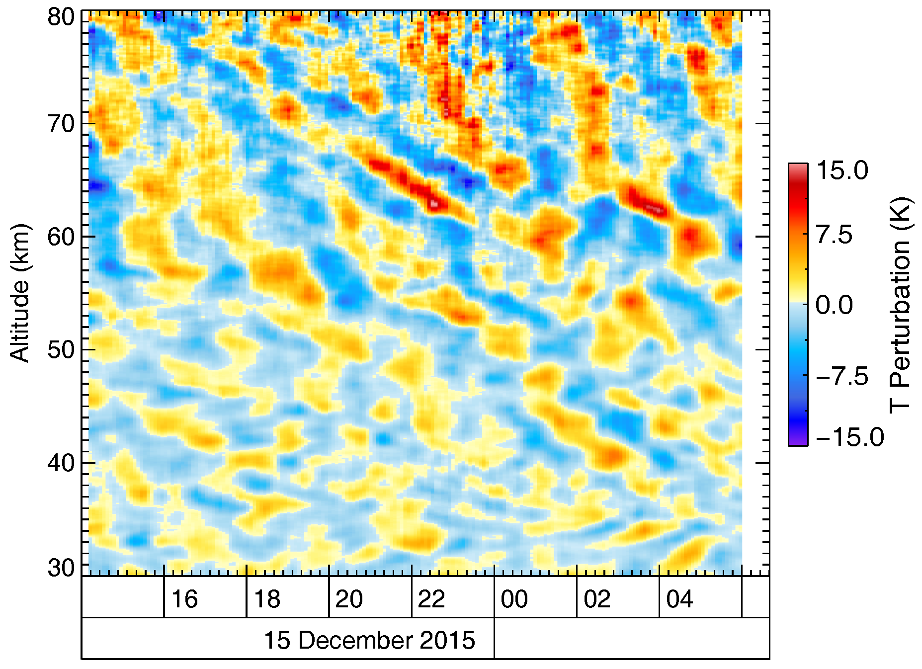
2. Gravity Wave Signatures in Ground-Based Lidar Data

Lidar is still the only technology allowing temperature measurements with sufficiently high vertical and temporal resolution in the stratosphere and mesosphere. In order to retrieve gravity wave-induced temperature perturbations, the lidar measurements are usually decomposed into a local background and perturbations around this background. Signatures of gravity waves are then defined as the observed temperature minus the background, i.e., the perturbations. A common method to compute the background is applying spectral filters to the observational data [20]. Figure 1 shows an example of lidar data filtered with a 3 h running mean. It is important to note that the filter limits the sensitivity to gravity waves within a range of periods between approximately 1 and 5 h. In the real atmosphere, at any given time, the lidar observes a superposition of a multitude of different wave packets with different periods, vertical wavelengths and amplitudes. Depending on the characteristics of the filter, different parts of the gravity wave spectrum become visible [20].
As the human brain is very good at identifying patterns, it comes into one’s mind to connect the individual colored patches of red and blue in Figure 1 and form phase lines descending in time. The next step, identifying the phase lines as quasi-monochromatic gravity waves, appears natural. However, in doing so, it is easy to overlook sudden jumps, which disturb the “nice” phase line patterns. For example, around 03 UTC, the phase line becomes suddenly almost vertical above a 65 km altitude. In fact, these jumps suggest that we should detach ourselves from the simple and perspicuous conception of monochromatic waves and think of wave packets instead.

3. Basic Considerations

3.1. Plane Boussinesq Waves

In order to demonstrate what kind of phase lines one can expect from internal gravity waves observed at a fixed location, we consider the propagation of plane 2D Boussinesq internal waves in a uniformly stratified, nonrotating fluid with zero mean flow. The respective governing equations and the derivations of the dispersion and polarization relationships are outlined in detail in Sutherland [29] (Chapter 3.3). The vertical displacement field ξ ( x , z , t ) for a traveling wave, which was produced by some initial perturbation, is given by:
ξ ( x , z , t ) = A ξ cos ( k x + m z ω ^ t ) ,
where k and m are the real-valued horizontal and vertical wavenumbers k = ± 2 π / λ x and m = ± 2 π / λ z with the respective wavelengths λ x and λ z . Polarization relations to calculate other physical quantities of the wave solution (1) are provided by Sutherland [29] (Chapter 3.3) and Gill [30] (Chapter 6.5). The wave frequency ω ^ = 2 π / T (T is the wave period) is given by the dispersion relation for Boussinesq internal waves in the x-z-plane:
ω ^ 2 = N 2 k 2 k 2 + m 2 ,
where N is the buoyancy frequency determining the stably-stratified environment. As mentioned by Sutherland [29] (p. 155), it is convenient to require ω ^ to be positive. Thus, the signs of the components of the wavenumber vector k = k e x + m e z determine the direction of wave propagation, i.e., here: the direction of the propagation of the wave phase. A convenient way to express ω ^ is:
ω ^ = N cos φ
with:
φ tan 1 m k for π 2 φ + π 2 .
The quantity φ is the angle formed between the wavenumber vector k and the k-axis (see Sutherland [29] (Figure 3.2)). The other two meanings are: (i) φ is the angle formed between lines of constant phase and the z-axis; and (ii) the magnitude of φ determines the wave frequency ω ^ via Equation (3). Generally, the wavenumber vector k can point into the four quadrants of the k-m-diagram, and the sign of φ is determined by the signs of the components of k and m:
k A upward and leftward propagating phases : k < 0 , m > 0 φ < 0 k B upward and rightward propagating phases : k > 0 , m > 0 φ > 0 k C downward and leftward propagating phases : k < 0 , m < 0 φ > 0 , and k D downward and rightward propagating phases : k > 0 , m < 0 φ < 0 .
As in Whitham [31] (Equation (11.4)), we define the phase velocity c p according to:
c p ω ^ | k | k | k | .
Using the definition of the wave frequency ω ^ given by Equation (3), we obtain:
c p x = N k cos 3 φ and c p z = N k cos 2 φ sin φ
as the two components of the vector c p in the x- and z-directions; see Sutherland [29] (Equation (3.60)). As illustrated and discussed by Sutherland [29] (Figure 1.25), c p = | c p | = ω ^ | k | is the velocity of an observer sitting on the crest (or trough) of the wave measures with respect to ground.
Alternatively and especially important for analyzing vertical time series of atmospheric profile measurements taken at a fixed location, the quantity:
c P z = ω ^ m
is the vertical speed of crests moving past the observational site. Actually, combining Equation (7) with the dispersion relationship (3), one obtains:
c P z = N m cos φ = N k cos φ cot φ
from which the phase angle φ can be determined from observed vertical time series of atmospheric variables. The slope of the phase lines in vertical time series is equal to c P z . In a similar way, also:
c P x = ω ^ k
can be calculated. The slope of the phase lines in a horizontal time series taken at fixed altitude is equal to c P x . For the 2D Boussinesq waves, we obtain using Equations (3) and (4):
c P x = N k cos φ = N m sin φ .
It does not make sense to compute a vector c P from the components c P x , c P y and c P z , because | c P | is not equal to | c p | for 2D or 3D waves. This equality holds only for one-dimensional waves. Finally, we define the group velocity vector as:
c g ω ^ k e x + ω ^ m e z
which gives for 2D internal Boussinesq waves the following components of c g in the x- and z-directions:
c g x = ω ^ k = N k sin 2 φ cos φ , and
c g z = ω ^ m = N k cos 2 φ sin φ = c p z .
The above Equations (12) and (13) are identical to Equation (6.6.1) of Gill [30] for 2D internal waves.
Figure 2 shows the components of the phase velocities c p x and c p z and group velocities c g x and c g z for selected, fixed values of the vertical wavenumber m (vertical wavelengths λ z ) as a function of the phase angle φ. Therefore, Equation (6) must be rewritten as:
c p x = N m cos 2 φ sin φ and c p z = N m cos φ sin 2 φ
and Equations (12) and (13) as:
c g x = N m sin φ sin 2 φ and c g z = N m cos φ sin 2 φ = c p z .
As expected from the above equations, the horizontal phase velocities c p x are positive for the wave vector orientations k B and k C and negative for k A and k D , respectively. The horizontal component of the phase velocity c p x is zero for φ = 0 and for | φ | = 90 and attains maximum/minimum values if | φ | = sin 1 1 / 3 35 , as depicted in Figure 2a. According to the above equations, the horizontal components of the group velocity c g x have for fixed values of m the same sign-dependence on φ as c p x . The horizontal group velocity c g x is zero if φ = 0 and reaches maximum/minimum values of N / m for | φ | 90 . The vertical components of the phase and group velocities c p z and c g z are zero for waves with φ = 0 and | φ | = 90 . The extrema of c p z and c g z are attained if | φ | = tan 1 2 ≈ 55 , as shown in Figure 2b. Figure 2c illustrates the sin ( φ ) - and cos ( φ ) -dependences of c P x and c P z according to Equations (8) and (10), respectively.

3.2. Wave Packets

In textbooks, dispersive waves are often introduced by superpositions of plane waves with nearly equal wavenumbers and frequencies, e.g., Gill [30] (Chapter 5.4). In general, the resulting wave packets are sinusoidal in phase k x + m z ω ^ t , but with an amplitude varying from place to place and time to time. It can be shown that the resulting amplitude is a function of x c g t only, e.g., Gill [30] (Chapter 6.6). In order to illustrate the peculiarity of internal gravity waves (in contrast to water waves and Rossby waves), that the group propagation is perpendicular to the phase propagation, we replace the constant amplitude A ξ in Equation (1) by:
A ˜ ξ ( x c g x t , z c g z t , t ) = A ξ exp x x 0 c g x t 2 σ x 2 + ( z z 0 c g z t ) 2 σ z 2
where ( x 0 , z 0 ) determines the initial position of the wave packets’ center at time t = 0, and c g x and c g z are the components of the group velocity given by Equations (12) and (13). The variances σ x and σ z determine the width and the depth of the wave packet.

3.3. Doppler Shift

So far, we considered the propagation of 2D internal Boussinesq waves in a nonrotating fluid with zero mean flow U = 0 . If we assume an altitude- and time-independent flow and U = const. Either positive or negative, the vertical displacement field ξ ( x , z , t ) can be written as:
ξ ( x , z , t ) = A ˜ ξ cos k ( x U t ) + m z ω ^ t ,
this means for an observer moving with the velocity U, the same vertical displacement as given by Equation (1) would be sensed. Rearranging Equation (15) gives:
ξ ( x , z , t ) = A ˜ ξ cos k x + m z ( ω ^ + U k ) t .
Now, we define the ground-based wave frequency:
ω = ω ^ + U k
in accordance with the terminology by Gill [30] (Equation 8.8.30) and Fritts and Alexander [27] (Section 2.1). In some text books (e.g., Nappo [32] (Chapter 2) or Sutherland [29] (Chapter 6.2)), Ω is used instead of ω ^ to denote the intrinsic wave frequency, which satisfies the dispersion relation for stationary waves Equation (3). The Doppler-shifted wave frequency ω is the frequency observed in a fixed coordinate system, i.e., the ground-based frequency. An immediate consequence of Equation (17) is:
c g x = ω k = U + N k sin 2 φ cos φ ,
while the vertical component of the group velocity c g z remains unchanged.

3.4. Illustrations

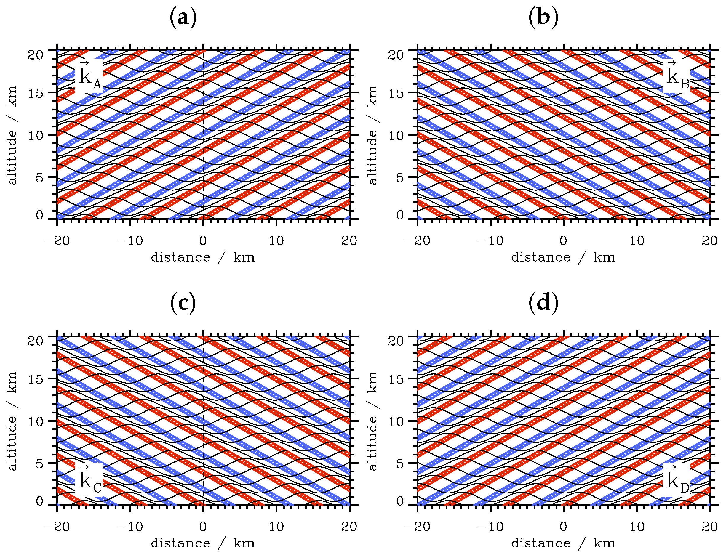
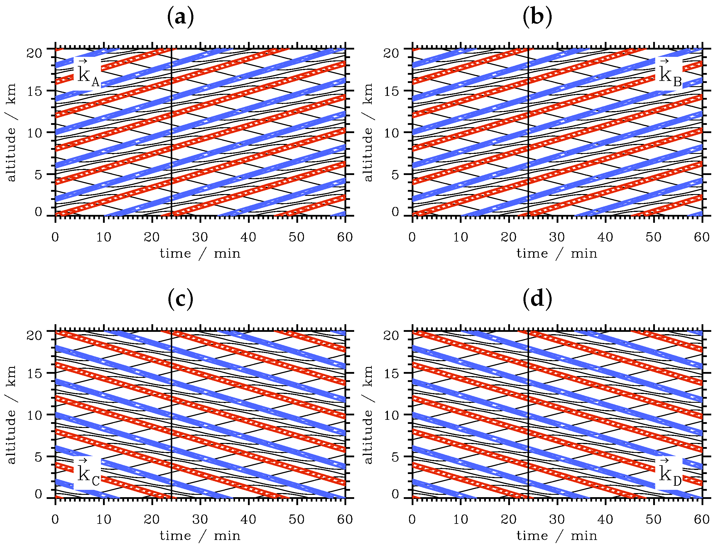
3.4.1. Plane Waves in an Atmosphere with Zero Wind

Cases of phase propagation are shown in Figure 3 and Figure 4. Here, the wavenumber vectors k A , k B , k C and k D determine the four possible directions of phase propagation in the x-z-plane (see Table 1 for the specific values). The spatial snapshots show the wave fronts according to the given directions of the wave vectors, which are normal to the phase lines (Figure 3). The time series recorded along the lines drawn in Figure 3 show upward sloping phase lines for the upward pointing wavenumber vectors k A and k B (Figure 4a,b) and downward sloping phase lines for the downward pointing wavenumber vectors k C and k D (Figure 4c,d). These slope orientations and slope angles are independent of the direction of the horizontal phase propagation.
If we do not know the given characteristics of the plane gravity waves as listed in Table 1, how much information about the waves can be obtained by analyzing the time series only? First of all, from the distance between troughs or ridges in Figure 4, the vertical wavelength λ z , hence, the vertical wavenumber m can be determined. Via the recorded period T = 2 π / ω , we obtain the ground-based frequency ω, which is equal to the intrinsic frequency ω ^ in the case of zero wind. The slope of the phase lines gives the apparent vertical phase speed c P z = ± λ z / T , and via an estimate of the background stratification N, the phase angle φ can be estimated from Equation (8). Either Equation (4) or Equation (2), rewritten as:
k = ± m N 2 ω 2 1
can be used to calculate an estimate of the horizontal wavenumber components k for internal Boussinesq waves. This means, all of the wave parameters can be determined quite easily. Unfortunately, the slopes of phase lines in Figure 4 cannot provide any information about the horizontal propagation direction. Therefore, the sign of k in the above equation is undetermined. The outlined approach is fine as long as the atmosphere is at rest. Before we consider the impact of a mean wind, we illustrate the results for wave packets in the next section.

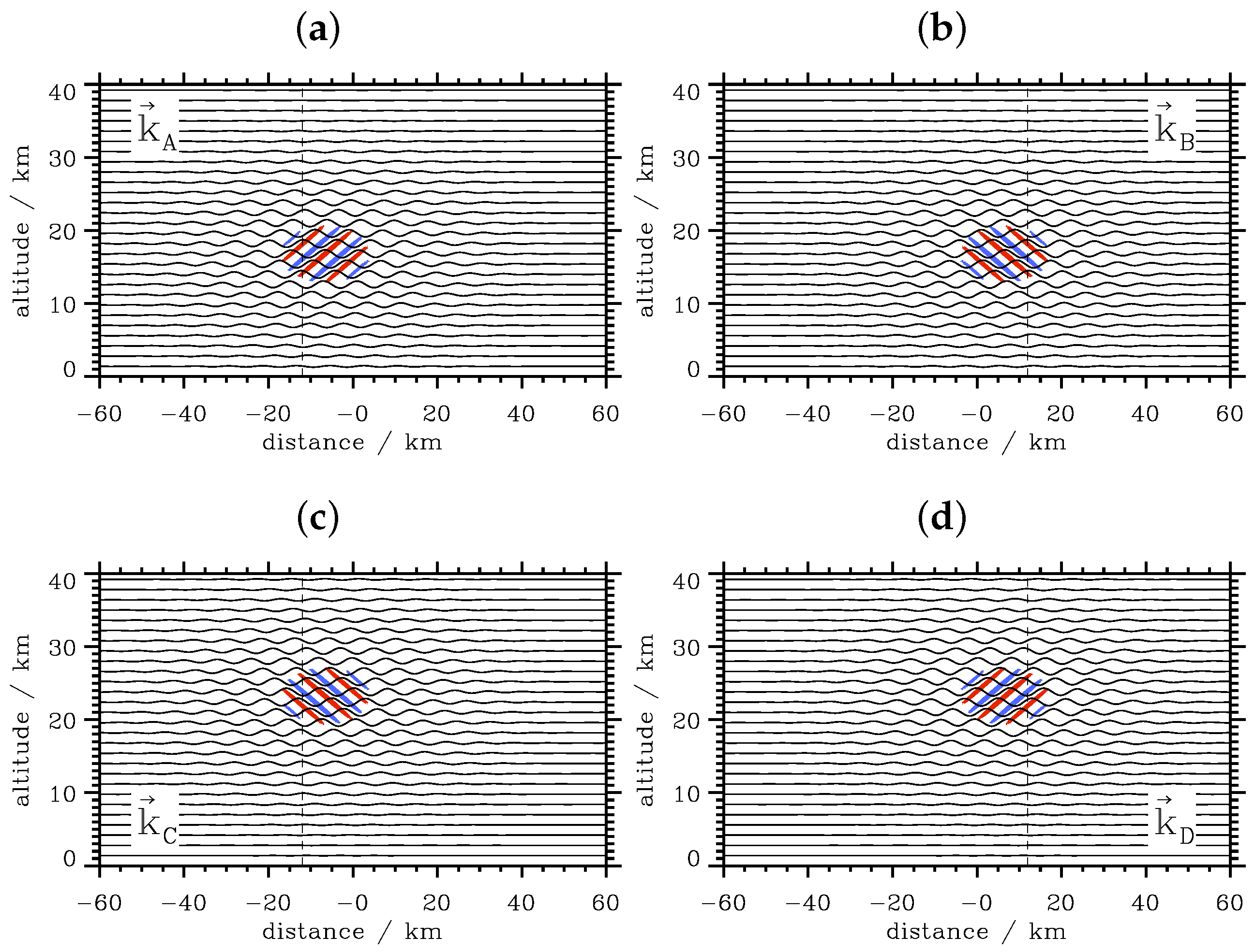
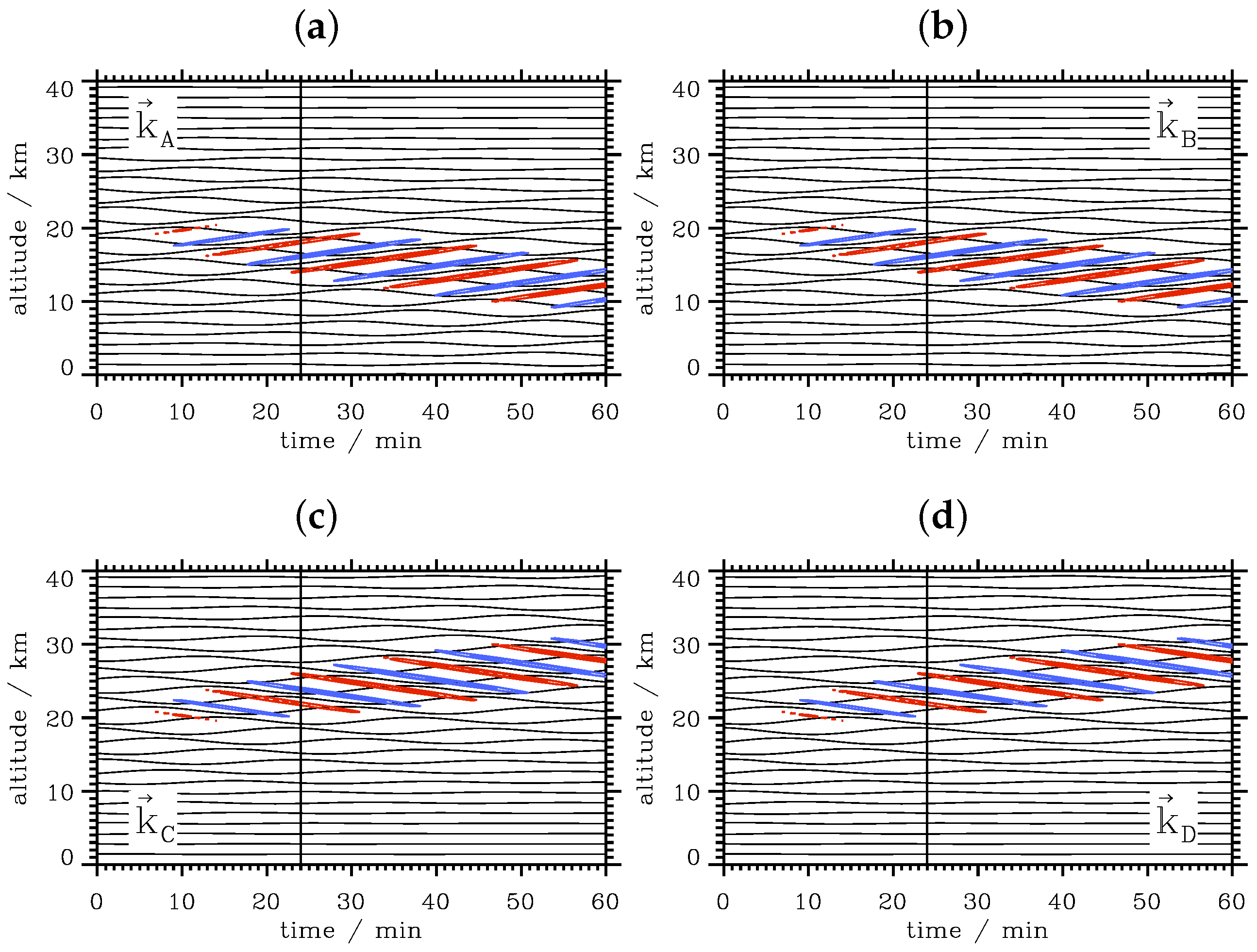
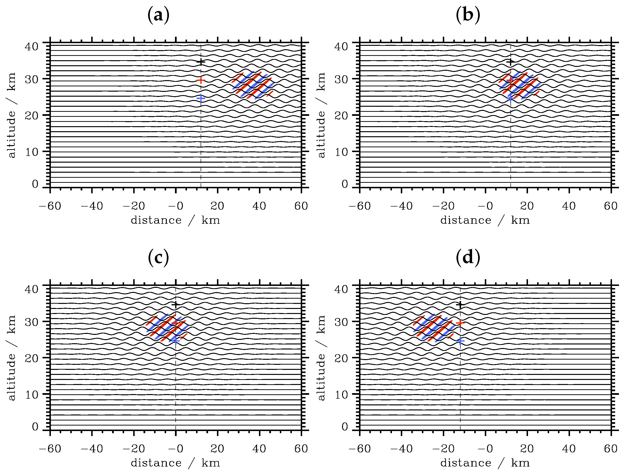
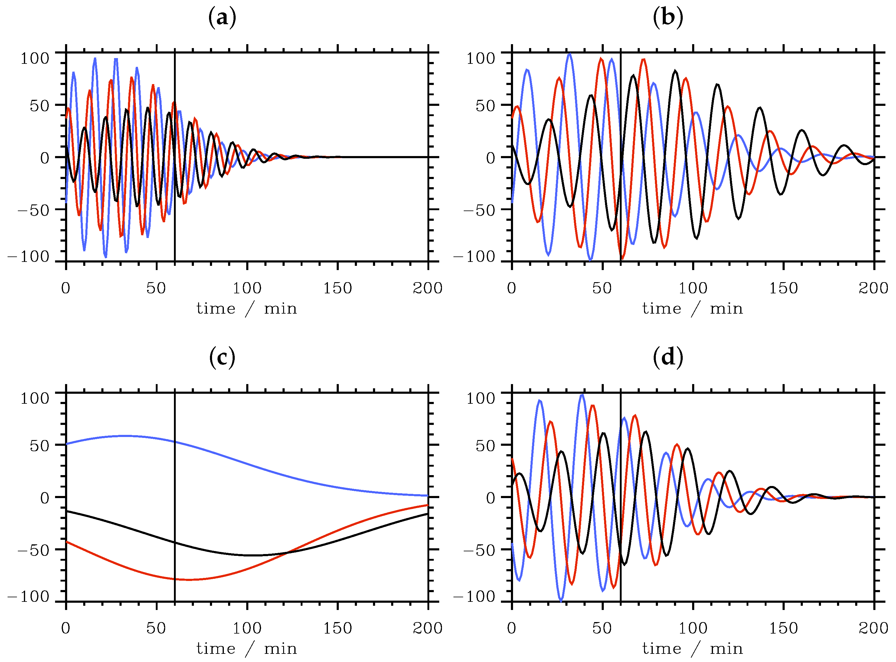
3.4.2. Wave Packets in an Atmosphere with Zero Wind

Figure 5 illustrates the spatial snapshots of vertical displacements ξ ( x , z , t ) for wave packets with group velocity components c g x and c g z as given by Equations (12) and (13) for the same k- and m-values from the former section (Table 1). The width and depth of the wave packets are given by the variances σ x = 32 km and σ z = 12 km, respectively. The orientations of the phase lines in Figure 5 are the same as for the plane waves as shown in Figure 3. Now, and due to the localized wave packets, the phase lines are restricted to a smaller area, as expected. The wave packets propagate with the group velocity | c g | vertically and horizontally away from their initial center point ( x 0 , z 0 ) = (0, 20 km): the upper row wave packets propagate downward; the bottom row wave packets propagate upward; the left column wave packets propagate leftward; the right column wave packets propagate rightward (Figure 5).
The altitude time plots as shown in Figure 6 depict the same orientation of phase lines as the plots for plane waves: downward propagating wave packets manifest themselves as upward sloping phase lines (Figure 6a,b) and upward propagating wave packets as downward sloping phase lines (Figure 6c,d). It is typical for these dispersive waves that the wave pattern is also limited in vertical space and time.
Again, we ask: What information of the wave characteristics can be obtained from the time records without knowing the given values for k and m? As in the previous section, the vertical distance between troughs or ridges in Figure 6 gives the vertical wavelength λ z and wavenumber m. Assume the observational time is long enough that the complete wave packet propagates horizontally through the observational volume. Then, the recorded period T = 2 π / ω can be used to obtain an estimate of the ground-based frequency ω. In such a case, the slope of the phase lines gives the vertical phase speed c P z = ± λ z / T and the propagation directions of the wave phases and of the wave packet, respectively. Using an estimate of the background stratification N, the phase angle φ can be estimated from Equation (8) and k can be computed. Technically, the Equations (12) and (13) can now be employed to derive the components of the group velocity c g x and c g z from the known values of k, m, and φ.
Summarizing the assumptions involved so far if we would like to retrieve wave properties from the virtual time series observations as presented in Figure 6:
(a)
the observed phase lines belong to a spatially- and temporally-localized wave packet,
(b)
the observed phase lines allow the graphical determination of the vertical wavelength λ z and of the ground-based frequency ω,
(c)
the observed waves obey a dispersion relation for internal Boussinesq wave like Equation (3),
(d)
the background stratification N is nearly constant over an altitude range of at least one vertical wavelength λ z and can be computed from the observation or meteorological data and
(e)
there is no mean wind in the atmosphere.
The latter assumption will be abolished in the next section.

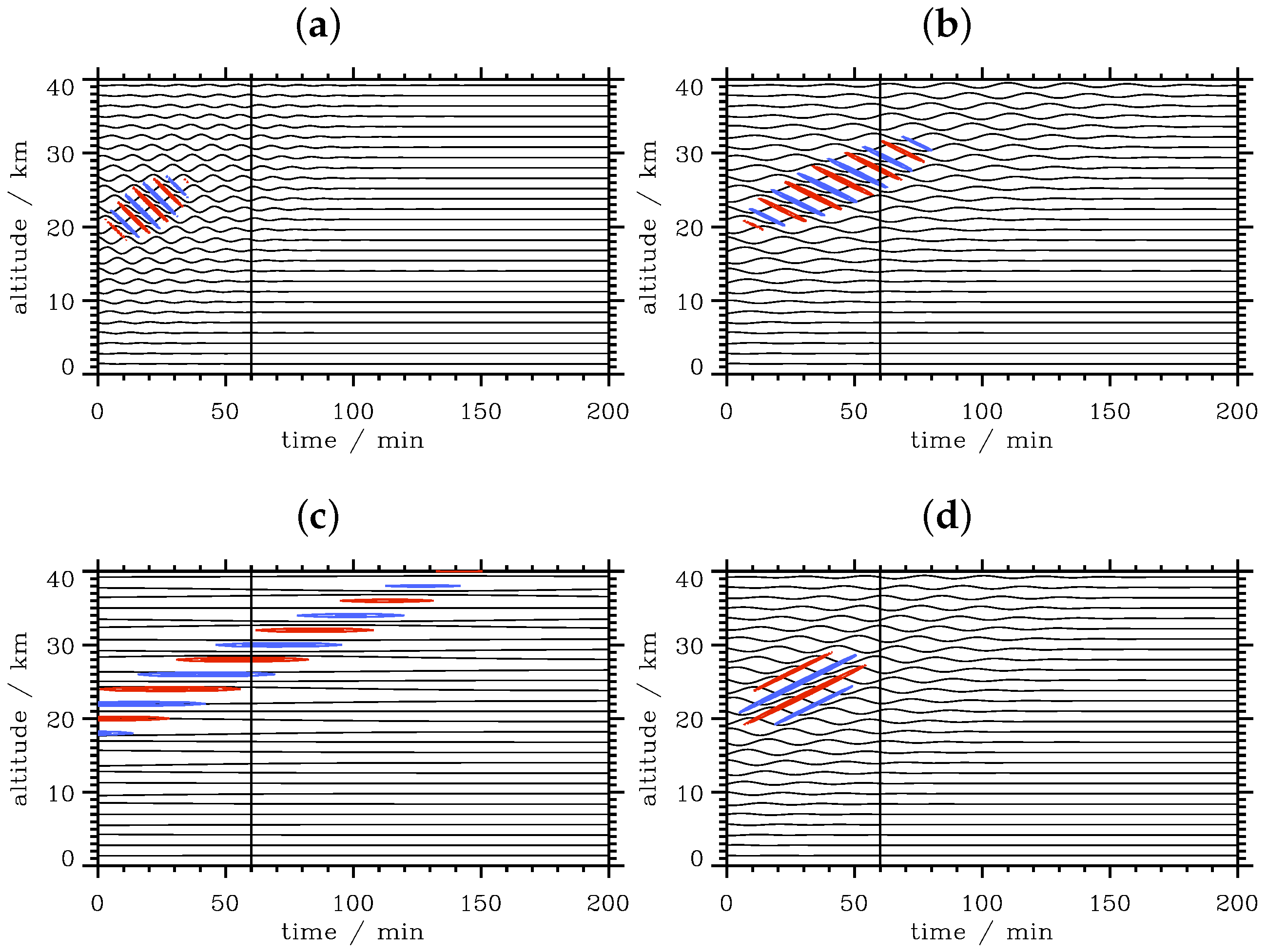
3.4.3. Doppler-Shifted Wave Packets

Here, we consider upward propagating wave packets. For this purpose, we select wave packets with the wavenumber vector k D (Panel (d) in Figure 5 and Figure 6) to investigate the impact of a uniform mean wind on the orientation of phase lines in the virtual vertical time series. The spatial snapshots of the vertical displacements ξ ( x , z , t ) for four different mean velocities U = 0, ± c P x and 2 c P x are depicted in Figure 7.
As the vertical group velocity c g z is not impacted by the Doppler shift, all wave packets propagate vertically by the same amount. However, the magnitudes and directions of horizontal propagation differ as a function of U, as expected from Equation (18) (Figure 7). Figure 8 depicts the vertical time series of the four cases: the phase lines for U = c P x (Figure 8a) are compressed compared to the case U = 0 (Figure 8b). Yet, the orientation of the phase lines is the same: upward propagating wave packets exhibit downward sloping phase lines in the vertical times series. The situation changes if U c P x as shown in Figure 8c,d: for U = c P x , the phase lines appear as horizontal lines, and for U = 2 c P x , the phase lines swapped the orientation and slope upward. Thus, the magnitude and the direction of the mean wind alter the phase orientation of the recorded time series considerably. This Doppler shifting may lead to an erroneous interpretation if no other (spatial or wind) information is provided. Especially, Figure 8c reveals that horizontal phase lines can be misinterpreted as stationary mountain waves if U = c P x . Furthermore, the recorded time series at the three selected altitude levels as shown in Figure 9 indicate that the estimate of a ground-based wave frequency ω is heavily influenced by the magnitude and direction of the mean wind. Without additional information, only the vertical wavelength λ z can be determined from the vertical time series.

4. Idealized Numerical Simulations

In this section, we consider the 2D vertical propagation of mountain waves in different regimes depending on the horizontal scale of the obstacle. The numerical simulations are conducted for small-amplitude gravity waves, so nonlinear effects are omitted from the discussion. The main focus is on providing virtual vertical time series above and in the lee of the mountains. These profiles will be interpreted, and conclusions are drawn with respect to patterns found in real atmospheric ground-based lidar measurements.

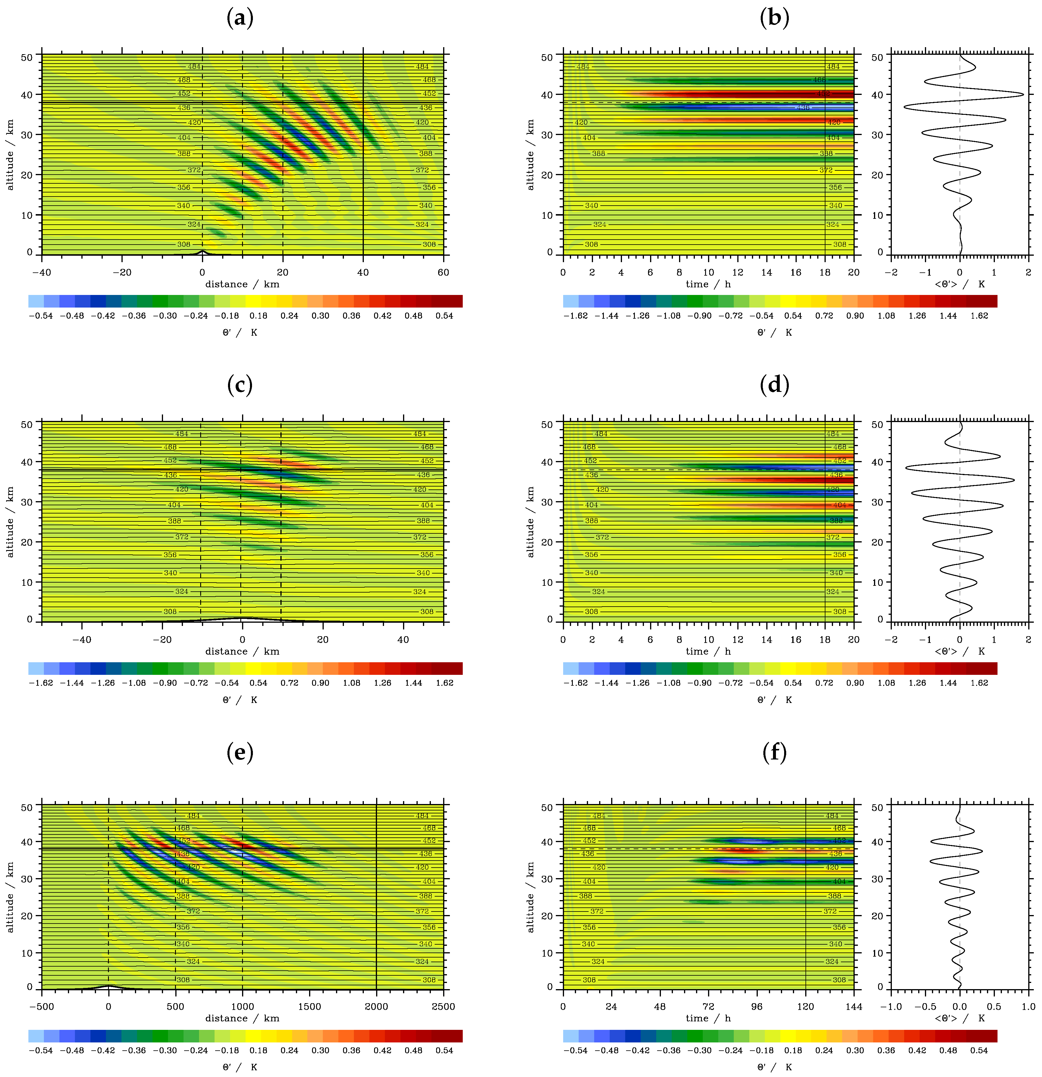
4.1. Archetypal Regimes of Vertically-Propagating Internal Gravity Waves

In contrast to the free internal waves, which were generated by some initial perturbation (see previous Section 3), the waves being studied in this section are forced waves. Here, we consider internal gravity waves in a stably-stratified, isothermal atmosphere ( N = const.), which are excited by a uniform flow U over small-amplitude mountains, so that the atmospheric wave response is quasi-linear. These orographically-excited gravity (mountain) waves have a continuous source of energy. Due to the upward and downwind radiation of wave energy in the numerical model, these small-amplitude waves become stationary after a certain time, and the simulated wave patterns do not move with respect to the ground. Therefore, the intrinsic frequency ω ^ = U k , i.e., the ground-based frequency is zero, and the waves follow the modified dispersion relation (3):
ω ^ 2 = N 2 cos 2 φ + f 2 sin 2 φ = N 2 k 2 k 2 + m 2 + f 2 m 2 k 2 + m 2 ,
where the Coriolis parameter f allows us to study gravity waves influenced by Earth’s rotation. To discuss Equation (19), it is useful to introduce the aspect ratio α of the vertical to the horizontal scale of the excited waves,
α k m = cot φ .
From Equation (19), a unique relation between ω ^ and α can be derived:
α 2 = ω ^ 2 f 2 N 2 ω ^ 2
According to Gill [30] (Chapter 8.4), three major wave regimes archetypal for a large class of mountain waves can be distinguished. Based on the magnitude of α, the wave regime f ω ^ N will be divided into the:
(i)
non-hydrostatic wave regime, the
(ii)
hydrostatic “nonrotating” wave regime and the
(iii)
hydrostatic “rotating” wave regime.
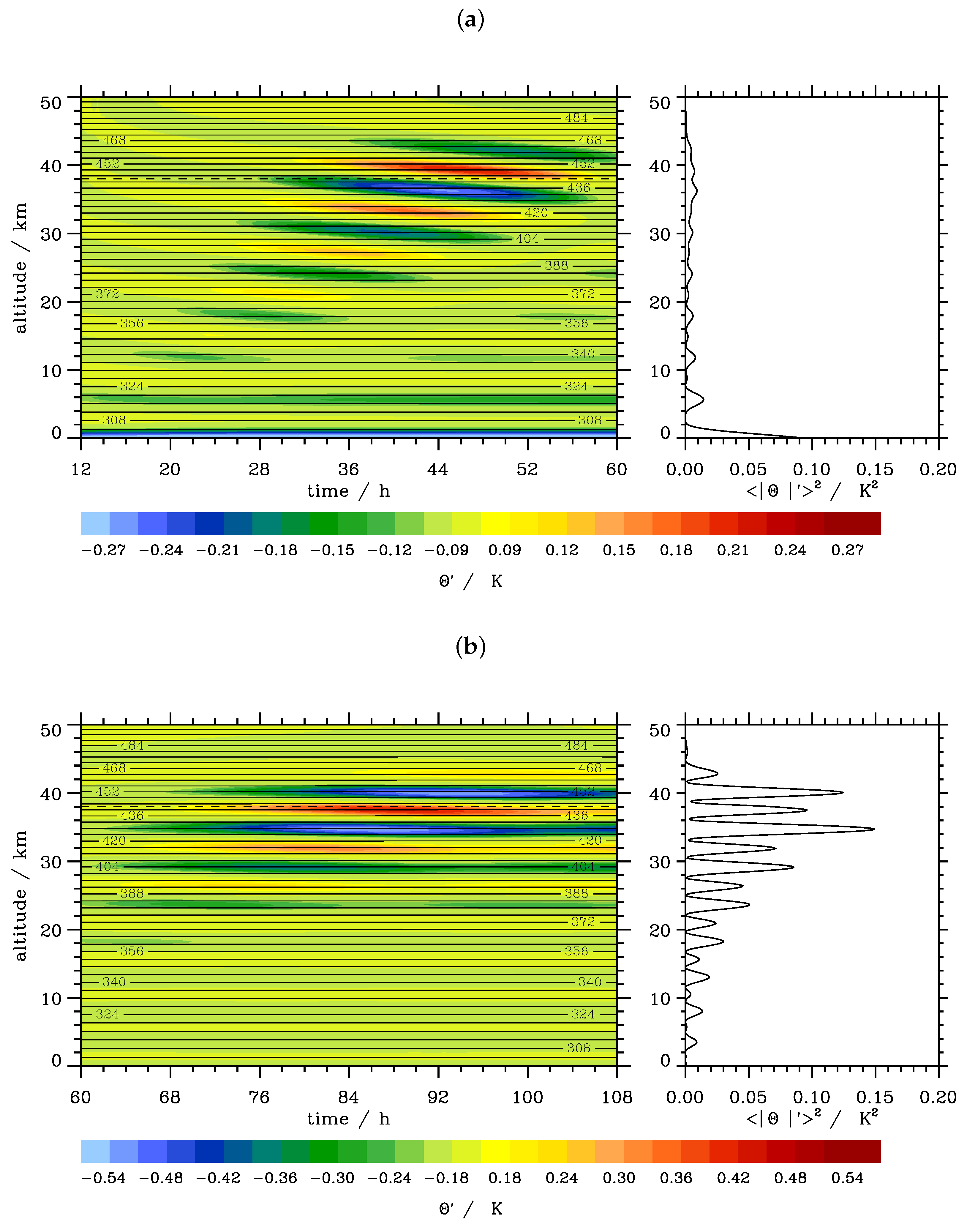
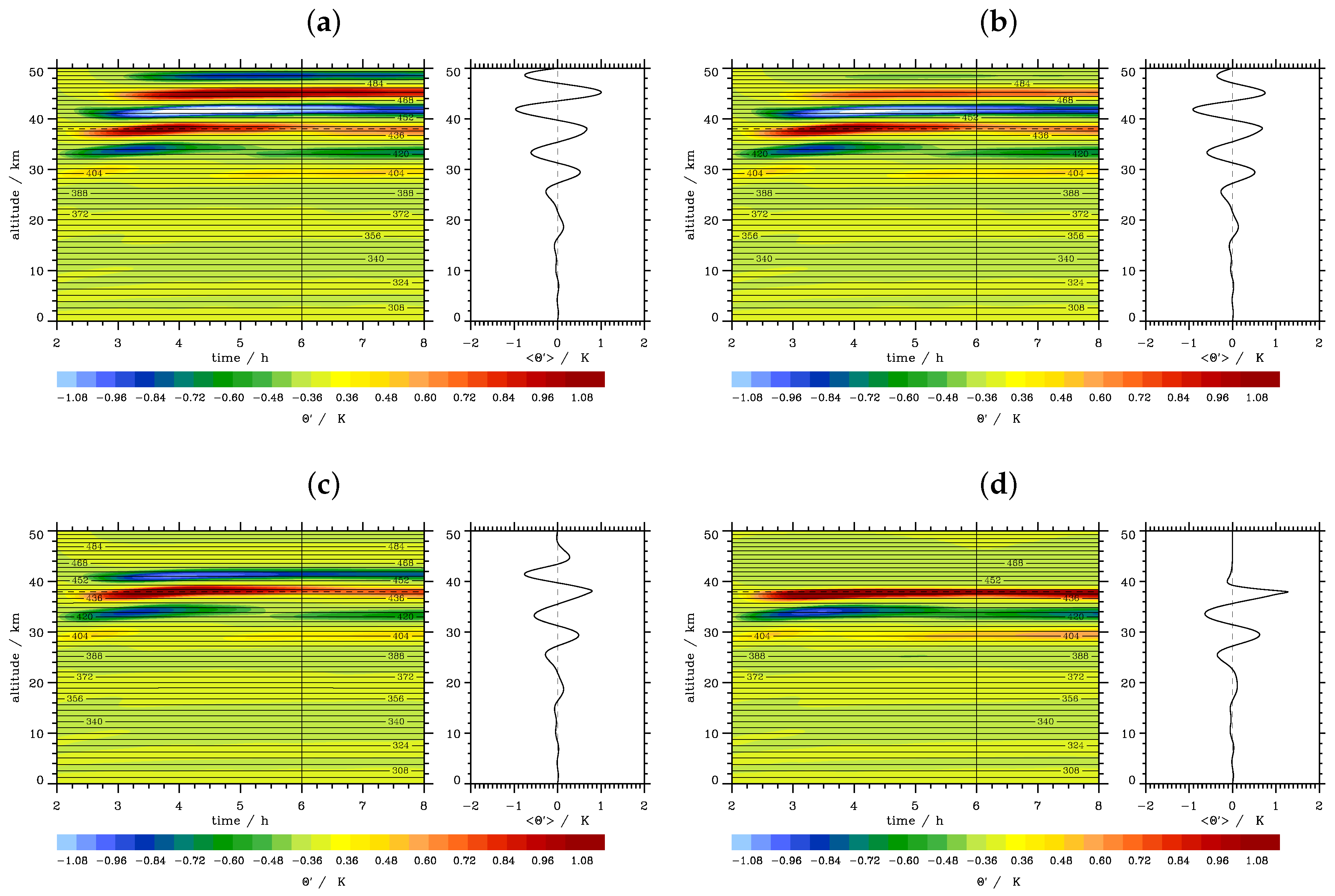
Regime (i) is characterized by waves with frequencies ω O ( N ) , but ω N . These waves are high-frequency, nonhydrostatic gravity waves. To excite such waves, the width of the mountain L must be small, in the order of U / N , i.e., L 1 km for typical tropospheric values of U = 10 m·s 1 and N = 0.01 s 1 . The resulting internal waves have an aspect ratio α of the order of one or larger: α O ( 1 ) . Thus, the vertical wavenumber m has the same size as k, and the vertical wavelength in this wave regime is λ z 2 π / | m | . The vertical wavenumber is determined by Equation (3) and amounts to m 2 = k c 2 k 2 , where the cutoff wavenumber is defined as k c = N / U , whereby k c > k for vertically-propagating waves. The intrinsic horizontal group velocity c g x = N / m 1 + α 2 3 / 2 depends on the vertical wavenumber m; see Figure 2a. The group velocity relative to the ground for a single wave component is upward and downwind in the direction of the wavenumber vector k and varies between the vertical direction ( k = 0 ) and the horizontal downwind direction (k = k c ), [30] (Chapter 8.8).
Regime (ii) is defined as the range of frequencies for which f ω ^ N. The dispersion relation (19) for “nonrotating” hydrostatic waves can be approximated for small values of α as ω ^ 2 = N 2 α 2 . Therefore, this regime is equivalent to the range of aspect ratios α given by f / N α ≪ 1. Typically, N / f is of the order 100, so rotation does not affect wave propagation, hence the name “nonrotating”. From the approximated dispersion relation, one immediately sees that the vertical scale m 1 U / N . In contrast to the non-hydrostatic regime, it does not depend on the wavenumber k. This interesting result is a consequence of the dispersion relation and the hydrostatic assumption (typical horizontal scales are larger than the vertical scale). Therefore, the horizontal scale of the obstacles must be large: L U / N . A further consequence is the following set of relations for the components of the group velocity and their ratio:
c g x = N m , c g z = N m 2 k , and c g z c g x = α .
For upward propagating mountain waves (m = N / U ), the ground-based group velocity is c g x = U + N / m = U + N / ( N / U ) = 0; this means the waves propagate predominantly vertically and will be found directly above the obstacle.
Regime (iii) is defined as the range of frequencies for which ω ^ is of the order of f, but clearly ω ^ f. According to Equation (21), this is equivalent to the range of aspect ratios α f / N . In this hydrostatic “rotating” wave regime, the dispersion relation (19) can be approximated as:
ω ^ 2 f 2 + N 2 α 2 .
The horizontal scale of the obstacles is L U / | f | . As in the non-hydrostatic regime, the vertical scale m 1 depends on the horizontal wavenumbers according to m 2 = k c 2 k 2 1 f 2 / ( k 2 U 2 ) 1 . Therefore, m is again of the order U / N as the horizontal scale k 1 is much larger than in Regime (ii). The intrinsic horizontal group velocity is c g x = N 2 m 1 α N 2 α 2 + f 2 1 / 2 , and the vertical component c g z = α c g x . As α is very small, the ground-based horizontal group velocity is close to U. According to Equation (22), the wave energy is propagated upward and gains an increasing downwind component with decreasing α. The phase angle varies between 0 for k 1 = U / f and 90 for k. Waves excited in this regime are called low-frequency or inertia-gravity waves.

4.2. Results

The numerical simulations are conducted with the all-scale geophysical flow solver EULAG [33,34]. The governing equations and the numerical methods to solve them are sketched in the Appendix A. All simulations are run with n = 1280 grid points in the horizontal and l = 501 grid points in the vertical directions. The bell-shaped mountain profile is prescribed by z s ( x ) = h m / ( 1 + ( x / L ) 2 ) with the amplitude h m = 100 m and the mountain width L as listed in Table 2 for the three different wave regimes. We choose the atmospheric parameters U = 10 m·s 1 , N = 0.01 s 1 and f = 1.03·10 4 s 1 , as in the paper by Queney [35]; see also Gill [30] (Chapter 8.8). In effect, the characteristic Froude number F r = N h m / U = 0.1 < 1. Therefore, according to [36], we can expect that the steady nonlinear solution of the numerical simulations is close to the linear one. In the master thesis by H. Grogger (2016)2, the numerical solutions for the three wave regimes were compared with stationary analytic solutions for the uniform, stably-stratified flow over the small-scale bell-shaped mountain. The numerical and the analytic solutions were quantitatively very close as long as the amplitude of the mountain was small and the damping of the waves at the upper and lateral boundaries was reasonably treated.
At the upper and lateral boundaries, the vertical and horizontal radiation of wave energy is treated by relaxation terms in the governing Equations (A1) and (A2). The coefficients α ˜ and β ˜ are proportional to the inverse of the time scale τ. α ˜ and β ˜ are zero everywhere, except in the vicinity of the vertical and lateral boundaries where they increase linearly to one towards the model boundaries. The respective parameters for the numerical simulations are listed in Table 2.
Figure 10 shows the snapshots of the potential temperature fluctuations Θ superimposed by isentropic surfaces Θ at specific times and vertical time sections of these variables for the three wave regimes (i) to (iii). As expected from linear theory, the wave response for the non-hydrostatic regime is located above and downwind from the mountain (Figure 10a). As α ≈ 1, the phase angle is φ = 45 . This phase angle is simulated quite accurately by the model at an early stage (t ≈ 2 h) of wave propagation (Figure 10a). For φ = 45 , Equations (12) and (13) show that the horizontal and vertical group velocities c g x and c g z have the same magnitude (but opposite sign), which is about 3.5 m·s 1 for U = 10 m·s 1 . Therefore, the waves propagate both horizontally and vertically. Later, the following waves propagate into a disturbed environment, and the simulated phase angle becomes larger (not shown). After about 3 h (which is nearly the time the group needs to propagate 40 km vertically), the simulation achieves a stationary state, and the phase lines do not change altitude (Figure 10b). The vertical wavelength deduced from Figure 10b is about 6 km, which is close to the expected value of λ z = 2π km. The right panel in Figure 10b shows the time-averaged wave amplitude increasing nearly exponentially with height due to the decreasing background density ρ ¯ .
The hydrostatic “nonrotating” wave regime (ii) generates waves directly above the mountain; see Figure 10c. The phase angle φ of the simulated mountain waves is larger for this wave regime compared to the former regime (i) as the aspect ratio α = 0.1 is less than one. Please note, Figure 10a,c is plotted with the same length-to-height ratio of one, which allows a direct comparison of φ for the both regimes. The vertical time series for the hydrostatic “nonrotating” regime are shown directly above the top of the mountain (Figure 10d). Due to the smaller vertical group velocity c g z α U = 1 m·s 1 using Equation (22), the waves need about 11 h to propagate to an altitude of 40 km and to achieve a stationary state characterized by horizontal phase lines; see Figure 10d.
The hydrostatic “rotating” gravity waves have a much larger horizontal scale (estimated wavelength λ x ≈ 250 km from Figure 10e) compared to the mountain waves of the former regimes. The inertia-gravity waves are primarily simulated downwind of the mountain (Figure 10e). The Coriolis parameter affects the hydrostatically-approximated vertical group velocity c g z α U only marginally by a factor 1 − f 2 / ( k 2 U 2 ) . However, as α is an order of magnitude smaller than for the “nonrotating” wave regime, c g z ≈ 0.1 m·s 1 . Thus, the inertia-gravity waves take much longer (about five days) to reach an altitude of 40 km , as shown in Figure 10f. After that time, a nearly stationary state is attained, and the vertical wavelength is the same as in the former both regimes. From Equation (19), the following approximation of the horizontal group velocity c g x can be derived; see Gill [30] (Equation (8.4.24)):
c g x = α N 2 f 2 m N 2 α 2 + f 2 1 1 + α 2 3 / 2 α N 2 m N 2 α 2 + f 2 .
Thus, for α = 0 (k = 0), the group velocity is zero. As k increases, the group velocity c g x approximated for α ≪ 1 (the second term in the previous Equation (23)) results in c g x = α U γ (using m = N / U for our mountain waves) where γ is a factor of the order of O ( 1 ) . The horizontal group velocity is very small, and it cannot compensate the horizontal wind U. Therefore, the inertia-gravity waves propagate downwind much faster (three orders of magnitude) than they propagate vertically. It must be noted that the vertical scale in Figure 10e is strongly exaggerated, and the waves appear steeper than they are. As shown by [37], such waves can be observed in the stratosphere by airborne lidar measurements above and in the lee of the Scandinavian mountains.
The first conclusion from the presented results is that the wave response in ground-based lidar observations depends on the position where the lidar is located. Downwind of the mountain, mostly non-hydrostatic and inertia-gravity waves can be observed, whereas hydrostatic nonrotating waves dominate in close proximity to the mountain top. From the vertical time series of Θ (Figure 10), it is nearly impossible to differentiate between the different regimes as long as they are in a stationary state. Secondly, the time gravity waves require to propagate to the height of the observational volume of the virtual lidar varies strongly between the wave types. According to linear wave theory, gravity waves near the buoyancy cut-off k c propagate vertically fastest and the long inertial-gravity waves slowest. Estimates of the respective propagation times should be carefully considered for deducing potential source regions of the observed waves.
The numerical simulations also show a transient wave pattern. However, one should keep in mind that these transient states result from the response of the flow to the initial disturbance by introducing the mountain abruptly to a horizontally homogeneous background state Θ e ( z ) and u e = U, as well as from the interaction of the waves with the relaxation zone at the top of the computational domain. Figure 11 shows inertia-gravity wave packets propagating upward at two periods of the numerical simulations. At early times, the vertical times series show a phase tilt with downward phase propagation as expected for these upward propagating waves (Figure 11a). At later times, when the numerical simulations approach a stationary state, the tilt of the phase lines becomes smaller (Figure 11b). The time-averaged vertical profiles of < | Θ | > 2 show an interesting effect: when the phase lines are tilted, an averaging at constant altitudes leads to a cancellation of large Θ -contributions. This effect is not considered in the interpretation of the gravity potential energy density profiles E P < | Θ | > 2 derived from ground-based lidar observations. In other words: a decrease of E P at certain altitudes (as often observed) could also be caused by averaging over slanted phase lines. The effect is weaker the more the phase lines become horizontal; cf. Figure 11a,b.
A further effect is the reflection of gravity waves by the absorber layer at the top of the computational domain. The time scale τ z can be estimated as follows. If we assume an exponential decay of the solution in the relaxation zone ∝ exp z 2 / σ 2 , then the standard deviation is given by σ = 2 D τ z , where D is the diffusion coefficient. Now, we approximate D c g z L a b where L a b is the depth of the absorber layer, set σ = L a b and obtain for the time scale τ z L a b / 4 c g z . The time scales τ z listed in Table 2 are roughly based on this estimate. Figure 12 illustrates the effect of a decreasing time scale τ z on the numerical solutions in the vicinity of the absorber layer. First of all, the expected effect works: the magnitude of Θ decreases with increasing damping, i.e., decreasing τ z in the absorber layer. Secondly, the upward sloping phase lines appearing at early times directly beneath the absorber layer remain in all simulations. These transient patterns are obviously the result of the interaction of the wave packets arriving first at the sponge layer and becoming reflected from it. Afterwards, a steady state is established in the numerical solutions, which results from the balance of the forced orographically-induced waves and the damping in the absorber layer.

5. Conclusions

This paper shows three simple aspects that are essential by interpreting the vertical time series of ground-based lidar observations of middle atmosphere temperatures. First of all, all wave parameters, vertical wavelength λ z , period T and horizontal wavelength λ x , can be derived if an atmosphere with no wind would exist and a dispersion relation like Equation (3) can be assumed. Obviously, this is a pure theoretical result and has no obvious applications for real cases. However, one should keep in mind that the representation of phase lines as depicted in Figure 6 is often the basis of the interpretation of lidar observations: phase lines sloping upward are related to downward propagating waves (Figure 6a,b), and phase line sloping downward are related to upward propagating waves (Figure 6c,d). As mentioned in Section 2, it appears natural to associate the identified phase lines with quasi-monochromatic waves in the lidar observations (Figure 1). However, our simple consideration of wave packets shows that their appearance in vertical time series is discrete (Figure 8). Therefore, sudden jumps in the vertical time series could be a hint to detach ourselves from the simple and perspicuous conception of monochromatic waves and think of wave packets instead. It is the localization of wave packets in space and time in combination with the localized sounding volume that produces the complex pattern commonly seen in processed lidar data. With the exception of a few textbook cases, the patterns defy the monochromatic wave interpretation.
Considering a uniform mean wind U leads to the main conclusion of this study: depending on the magnitude of U, the orientation of the phase lines in the virtual lidar measurements changes due to the Doppler shift. For U c P x , the phase lines swap the slope, and the propagation direction can be easily misinterpreted. Thus, a careful determination of the horizontal phase propagation and the ambient wind is necessary to determine if waves seen in the ground-based lidar observations are propagating up- or down-ward in the ground-based lidar measurements.
The numerical simulations of a quasi-linear flow of small-amplitude mountains for three archetypal atmospheric wave regimes show a sensitivity of the virtual lidar observations on the relative position of the mountain and on its scale. In all three regimes, a stationary state is simulated, and the vertical time series show horizontal phase lines, as expected. Weakly non-stationary phenomena are simulated in the vicinity of the absorber at the top of the model. Here, the interaction of upward propagating waves with the sponge layer leads to reflected modes. The next step in our investigations will consider simulations with realistic wind and stability profiles and the analysis of time-dependent wind profiles.

Acknowledgments

Part of this research was funded by the German research initiative “Role of the Middle Atmosphere in Climate (ROMIC)” funded by the German Ministry of Research and Education in the project “Investigation of the life cycle of gravity waves (GW-LCYCLE, 01LG1206A)” and by the Deutsche Forschungsgemeinschaft (DFG) via the Project “Multiscale Dynamics of Gravity Waves” (FOR1898, MS-GWaves sub-projects GW-TP , DO1020/9-1, and PACOG, RA1400/6-1).

Author Contributions

Andreas Dörnbrack, Sonja Gisinger and Bernd Kaifler wrote the paper. Bernd Kaifler conducted the ground-based lidar measurements. Andreas Dörnbrack simulated the 2D flow over idealized topography.

Conflicts of Interest

The authors declare no conflict of interest.

Appendix A. Setup of the Numerical Simulations

The numerical simulations are conducted with the numerical model EULAG [33,34]. In our configuration, EULAG solves the anelastic equations for the Cartesian velocity components v = ( u , v , w ) Equation (A1), the potential temperature perturbations Θ = Θ − Θ e Equation (A2) and the continuity Equation (A3):
d v d t = G p ρ ¯ + g Θ Θ ¯ 2 Ω × v v e α ˜ v v e R v ,
d Θ d t = v · Θ e β ˜ ( Θ Θ e ) R Θ ,
· ρ ¯ v = 0 .
Here, d d t , and · represent the total derivative, the gradient and the divergence. The quantity p denotes the pressure perturbation with respect to the environmental state, g = ( 0 , 0 , g ) the gravitational acceleration and Ω the angular velocity of the Earth. The matrix G represents geometric terms, which result from the general, time-dependent coordinate transformation.
The potential temperature Θ ¯ ( z ) appearing in the dominator of the buoyancy term in Equation (A1), as well as the anelastic density ρ ¯ ( z ) in the mass continuity Equation (A3) refer to the hydrostatic reference state around a constant stability profile and are prescribed as:
ρ ¯ = ρ 0 exp z H ρ and Θ ¯ = Θ 0 exp N 2 g z
where H ρ = 7314 m is the density scale height and ρ 0 and Θ 0 are appropriate constants. For the numerical simulations conducted for this paper, the environmental state Θ e is set equal to Θ ¯ .
Furthermore, α ˜ ( v v e ) and β ˜ ( Θ Θ e ) represent relaxation terms, which enable the radiation of wave energy across the model boundaries. The symbol R Ψ denotes the right-hand side of the corresponding equations for the variables Ψ = (u, v, w, Θ ).
The name EULAG refers to the ability of solving the equations of motions either in an Eulerian (flux form) or in a semi-Lagrangian (advective form) ([33]) mode, solved via Equation (A4), with n denoting the time step and LE the corresponding semi-Lagrangian/Eulerian transport operator:
Ψ n + 1 = LE Ψ n + 1 2 Δ t R Ψ | n + 1 2 Δ t R Ψ n + 1
All simulations conducted for this paper use the Eulerian option by applying the multidimensional positive definite advection transport algorithm (MPDATA [38,39]). In general, EULAG owes its versatility to a unique design that combines a rigorous theoretical formulation in generalized curvilinear coordinates ([40]) with non-oscillatory forward-in-time (NFT) differencing for fluids built on MPDATA, which is based on the convexity of upwind advection ([34,38]) and a robust, exact-projection-type elliptic Krylov solver [34]. The flow solver has been applied to a wider range of scales simulating various problems, like boundary layer flow through complex geometries [41,42], baroclinic instability [43], gravity waves [44,45,46] or even solar convection [47]. Recently, the solver has been advanced to unstructured meshes; see [48].
The Equations (A1) and (A2) do not contain diffusion terms. The numerical simulations are yet stable as the NFT algorithm provides non-linear corrections of the original upwind scheme, an approach for high-resolution numerical schemes called implicit large-eddy simulation Grinstein et al. [49].

References

  1. Wilson, R.; Chanin, M.L.; Hauchecorne, A. Gravity waves in the middle atmosphere observed by Rayleigh lidar: 1. Case studies. J. Geophys. Res. Atmos. 1991, 96, 5153–5167. [Google Scholar] [CrossRef]
  2. Li, T.; She, C.Y.; Liu, H.L.; Leblanc, T.; McDermid, I.S. Sodium lidar observed strong inertia-gravity wave activities in the mesopause region over Fort Collins, Colorado (41° N, 105° W). J. Geophys. Res. Atmos. 2007, 112, D22104. [Google Scholar] [CrossRef]
  3. Lu, X.; Liu, A.Z.; Swenson, G.R.; Li, T.; Leblanc, T.; McDermid, I.S. Gravity wave propagation and dissipation from the stratosphere to the lower thermosphere. J. Geophys. Res. Atmos. 2009, 114, D11101. [Google Scholar] [CrossRef]
  4. Chen, C.; Chu, X.; McDonald, A.J.; Vadas, S.L.; Yu, Z.; Fong, W.; Lu, X. Inertia-gravity waves in Antarctica: A case study using simultaneous lidar and radar measurements at McMurdo/Scott Base (77.8° S, 166.7° E). J. Geophys. Res. Atmos. 2013, 118, 2794–2808. [Google Scholar] [CrossRef]
  5. Suzuki, S.; Lübken, F.-J.; Baumgarten, G.; Kaifler, N.; Eixmann, R.; Williams, B.P.; Nakamura, T. Vertical propagation of a mesoscale gravity wave from the lower to the upper atmosphere. J. Atmos. Sol. Terr. Phys. 2013, 97, 29–36. [Google Scholar] [CrossRef]
  6. Baumgarten, G.; Fiedler, J.; Hildebrand, J.; Lübken, F.-J. Inertia gravity wave in the stratosphere and mesosphere observed by Doppler wind and temperature lidar. Geophys. Res. Lett. 2015, 42, 10929–10936. [Google Scholar] [CrossRef]
  7. Ehard, B.; Kaifler, B.; Dörnbrack, A.; Preusse, P.; Eckermann, S.D.; Bramberger, M.; Gisinger, S.; Kaifler, N.; Liley, B.; Wagner, J.; et al. Horizontal propagation of large-amplitude mountain waves into the polar night jet. J. Geophys. Res. Atmos. 2017. [Google Scholar] [CrossRef]
  8. Chanin, M.L.; Hauchecorne, A. Lidar observation of gravity and tidal waves in the stratosphere and mesosphere. J. Geophys. Res. Oceans 1981, 86, 9715–9721. [Google Scholar] [CrossRef]
  9. Gardner, C.S.; Miller, M.S.; Liu, C.H. Rayleigh lidar observations of gravity wave activity in the upper stratosphere at Urbana, Illinois. J. Atmos. Sci. 1989, 46, 1838–1854. [Google Scholar] [CrossRef]
  10. Whiteway, J.A.; Carswell, A.I. Lidar observations of gravity wave activity in the upper stratosphere over Toronto. J. Geophys. Res. Atmos. 1995, 100, 14113–14124. [Google Scholar] [CrossRef]
  11. Whiteway, J.A.; Duck, T.J.; Donovan, D.P.; Bird, J.C.; Pal, S.R.; Carswell, A.I. Measurements of gravity wave activity within and around the Arctic stratospheric vortex. Geophys. Res. Lett. 1997, 24, 1387–1390. [Google Scholar] [CrossRef]
  12. Duck, T.J.; Whiteway, J.A.; Carswell, A.I. The gravity wave-arctic stratospheric vortex interaction. J. Atmos. Sci. 2001, 58, 3581–3596. [Google Scholar] [CrossRef]
  13. Rauthe, M.; Gerding, M.; Höffner, J.; Lübken, F.-J. Lidar temperature measurements of gravity waves over Kühlungsborn (54° N) from 1 to 105 km: A winter-summer comparison. J. Geophys. Res. Atmos. 2006, 111, D24108. [Google Scholar] [CrossRef]
  14. Yamashita, C.; Chu, X.; Liu, H.L.; Espy, P.J.; Nott, G.J.; Huang, W. Stratospheric gravity wave characteristics and seasonal variations observed by lidar at the South Pole and Rothera, Antarctica. J. Geophys. Res. Atmos. 2009, 114, D12101. [Google Scholar] [CrossRef]
  15. Alexander, S.P.; Klekociuk, A.R.; Murphy, D.J. Rayleigh lidar observations of gravity wave activity in the winter upper stratosphere and lower mesosphere above Davis, Antarctica (69° S, 78° E). J. Geophys. Res. Atmos. 2011, 116, D13109. [Google Scholar] [CrossRef]
  16. Ehard, B.; Achtert, P.; Gumbel, J. Long-term lidar observations of wintertime gravity wave activity over northern Sweden. Ann. Geophys. 2014, 32, 1395–1405. [Google Scholar] [CrossRef]
  17. Khaykin, S.M.; Hauchecorne, A.; Mzé, N.; Keckhut, P. Seasonal variation of gravity wave activity at midlatitudes from 7 years of COSMIC GPS and Rayleigh lidar temperature observations. Geophys. Res. Lett. 2015, 42, 1251–1258. [Google Scholar] [CrossRef]
  18. Kaifler, B.; Lübken, F.-J.; Höffner, J.; Morris, R.J.; Viehl, T.P. Lidar observations of gravity wave activity in the middle atmosphere over Davis (69° S, 78° E), Antarctica. J. Geophys. Res. Atmos. 2015, 120, 4506–4521. [Google Scholar] [CrossRef]
  19. Triplett, C.C.; Collins, R.L.; Nielsen, K.; Harvey, V.L.; Mizutani, K. Role of wind filtering and unbalanced flow generation on middle atmosphere gravity wave activity at Chatanika Alaska. Atmosphere 2017, 8, 27. [Google Scholar] [CrossRef]
  20. Ehard, B.; Kaifler, B.; Kaifler, N.; Rapp, M. Evaluation of methods for gravity wave extraction from middle-atmospheric lidar temperature measurements. Atmos. Meas. Tech. 2015, 8, 4645–4655. [Google Scholar] [CrossRef]
  21. Le Pichon, A.; Assink, J.D.; Heinrich, P.; Blanc, E.; Charlton-Perez, A.; Lee, C.F.; Keckhut, P.; Hauchecorne, A.; Rüfenacht, R.; Kämpfer, N.; et al. Comparison of co-located independent ground-based middle atmospheric wind and temperature measurements with numerical weather prediction models. J. Geophys. Res. Atmos. 2015, 120, 8318–8331. [Google Scholar] [CrossRef]
  22. Kaifler, B.; Kaifler, N.; Ehard, B.; Dörnbrack, A.; Rapp, M.; Fritts, D.C. Influences of source conditions on mountain wave penetration into the stratosphere and mesosphere. Geophys. Res. Lett. 2015, 42, 9488–9494. [Google Scholar] [CrossRef]
  23. Eliassen, A.; Palm, E. On the transfer of energy in stationary mountain waves. Geofys. Publ. 1961, 22, 1–23. [Google Scholar]
  24. Satomura, T.; Sato, K. Secondary generation of gravity waves associated with the breaking of mountain waves. J. Atmos. Sci. 1999, 56, 3847–3858. [Google Scholar] [CrossRef]
  25. Sato, K. Sources of gravity waves in the polar middle atmosphere. Adv. Polar Upper Atmos. 2000, 14, 233–240. [Google Scholar]
  26. Vadas, S.L.; Fritts, D.C.; Alexander, M.J. Mechanism for the generation of secondary waves in wave breaking regions. J. Atmos. Sci. 2003, 60, 194–214. [Google Scholar] [CrossRef]
  27. Fritts, D.C.; Alexander, M.J. Gravity wave dynamics and effects in the middle atmosphere. Rev. Geophys. 2003, 41. [Google Scholar] [CrossRef]
  28. Zhang, F.; Wang, S.; Plougonven, R. Uncertainties in using the hodograph method to retrieve gravity wave characteristics from individual soundings. Geophys. Res. Lett. 2004, 31, L11110. [Google Scholar] [CrossRef]
  29. Sutherland, B.R. Internal Gravity Waves; Cambridge University Press: Cambridge, UK, 2010; p. 394. [Google Scholar]
  30. Gill, A.E. Atmosphere-Ocean Dynamics; Academic Press: Cambridge, MA, USA, 1982; p. 662. [Google Scholar]
  31. Whitham, G.B. Linear and Nonlinear Waves; John Wiley and Sons: Chichester, UK, 1974; p. 636. [Google Scholar]
  32. Nappo, C.J. An Introduction to Atmospheric Gravity Waves, 2nd ed.; Academic Press: Cambridge, MA, USA, 2012; p. 400. [Google Scholar]
  33. Smolarkiewicz, P.K.; Margolin, L.G. On forward-in-time differencing for fluids: An Eulerian/Semi-Lagrangian Non-Hydrostatic Model for stratified flows. Atmos.-Ocean 1997, 35, 127–152. [Google Scholar] [CrossRef]
  34. Prusa, J.M.; Smolarkiewicz, P.K.; Wyszogrodzki, A.A. EULAG, a computational model for multiscale flows. Comput. Fluids 2008, 37, 1193–1207. [Google Scholar] [CrossRef]
  35. Queney, P. The problem of the airflow over mountains: A summary of theoretical studies. Bull. Am. Meteorol. Soc. 1948, 29, 16–26. [Google Scholar]
  36. Long, R.R. Some aspects of the flow of stratified fluids: I. A theoretical investigation. Tellus 1953, 5, 42–58. [Google Scholar] [CrossRef]
  37. Dörnbrack, A.; Birner, T.; Fix, A.; Flentje, H.; Meister, A.; Schmid, H.; Browell, E.V.; Mahoney, M.J. Evidence for inertia gravity waves forming polar stratospheric clouds over Scandinavia. J. Geophys. Res. Atmos. 2002, 107, SOL 30-1–SOL 30-18. [Google Scholar] [CrossRef]
  38. Smolarkiewicz, P.K.; Margolin, L.G. MPDATA: A finite-difference solver for geophysical flows. J. Comput. Phys. 1998, 140, 459–480. [Google Scholar] [CrossRef]
  39. Smolarkiewicz, P.K. Multidimensional positive definite advection transport algorithm: An overview. Int. J. Numer. Methods Fluids 2006, 50, 1123–1144. [Google Scholar] [CrossRef]
  40. Smolarkiewicz, P.K.; Margolin, L.O. On forward-in-time differencing for fluids: Extension to a curvilinear framework. Mon. Weather Rev. 1993, 121, 1847–1859. [Google Scholar] [CrossRef]
  41. Schröttle, J.; Dörnbrack, A. Turbulence structure in a diabatically heated forest canopy composed of fractal Pythagoras trees. Theor. Comput. Fluid Dyn. 2013, 27, 337–359. [Google Scholar] [CrossRef]
  42. Gisinger, S.; Dörnbrack, A.; Schröttle, J. A modified Darcy’s law. Theor. Comput. Fluid Dyn. 2015, 29, 343–347. [Google Scholar] [CrossRef]
  43. Kühnlein, C.; Smolarkiewicz, P.K.; Dörnbrack, A. Modelling atmospheric flows with adaptive moving meshes. J. Comput. Phys. 2012, 231, 2741–2763. [Google Scholar] [CrossRef]
  44. Prusa, J.M.; Smolarkiewicz, P.K.; Garcia, R.R. Propagation and breaking at high altitudes of gravity waves excited by tropospheric forcing. J. Atmos. Sci. 1996, 53, 2186–2216. [Google Scholar] [CrossRef]
  45. Smolarkiewicz, P.K.; Dörnbrack, A. Conservative integrals of adiabatic Durran’s equations. Int. J. Numer. Methods Fluids 2008, 56, 1513–1519. [Google Scholar] [CrossRef]
  46. Kühnlein, C.; Dörnbrack, A.; Weissmann, M. High-resolution Doppler lidar observations of transient downslope flows and rotors. Mon. Weather Rev. 2013, 141, 3257–3272. [Google Scholar] [CrossRef]
  47. Smolarkiewicz, P.K.; Charbonneau, P. EULAG, a computational model for multiscale flows: An MHD extension. J. Comput. Phys. 2013, 236, 608–623. [Google Scholar] [CrossRef]
  48. Smolarkiewicz, P.K.; Szmelter, J.; Xiao, F. Simulation of all-scale atmospheric dynamics on unstructured meshes. J. Comput. Phys. 2016, 322, 267–287. [Google Scholar] [CrossRef]
  49. Grinstein, F.F.; Margolin, L.G.; Rider, W. Implicit Large Eddy Simulation: Computing Turbulent Fluid Dynamics; Cambridge University Press: Cambridge, UK, 2007; p. 552. [Google Scholar]
  • 1.from B. Dylan: “One of us must know (sooner or later)”; Blonde On Blonde (1966).
  • 2.H. Grogger, Simulation of Deep Gravity Wave Propagation Using EULAG, Master Thesis, University of Innsbruck, 2017.
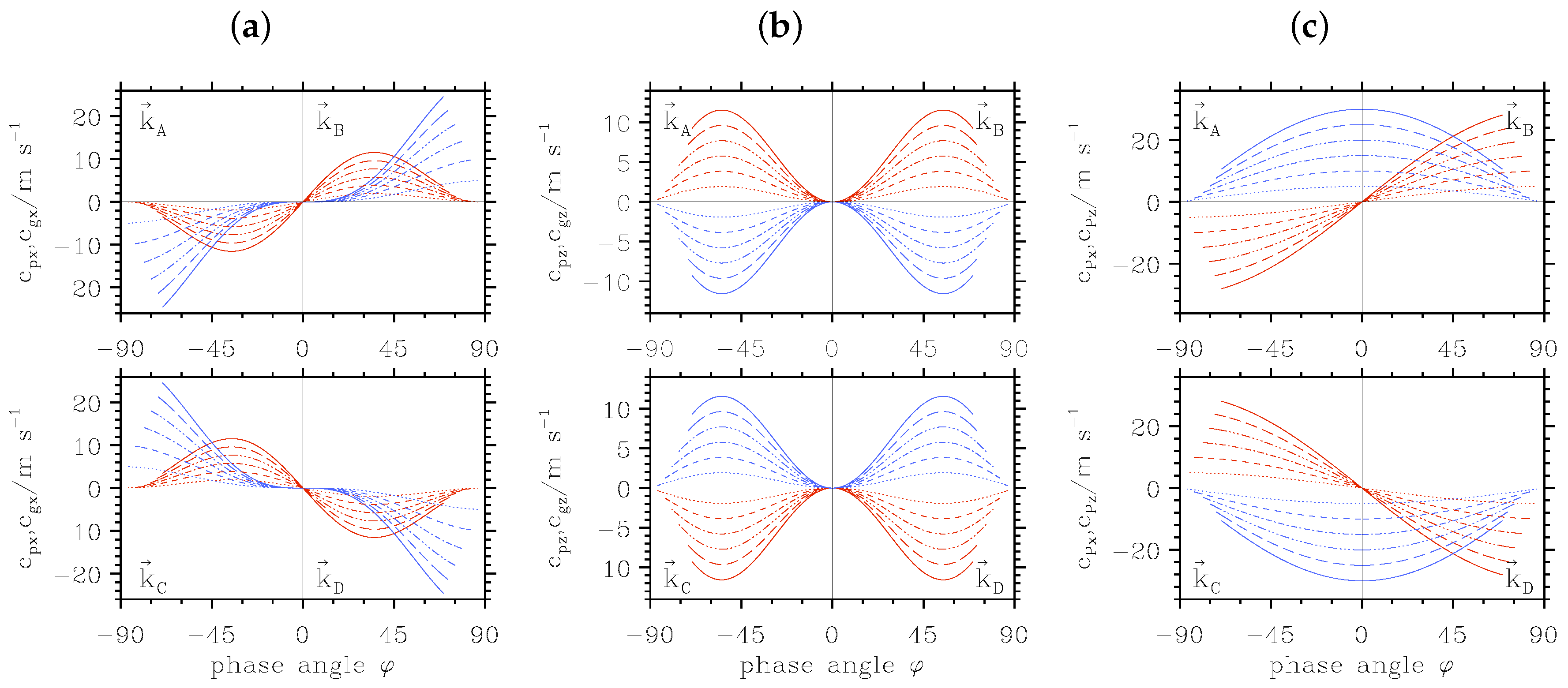
Figure 1. Gravity wave-induced temperature perturbations observed by Rayleigh lidar on 15/16 December 2015 above Sodankylä, Finland. The temperature measurements are filtered with a 3-h running mean to highlight signatures of gravity waves with periods in the range of approximately 1 to 5 h. The temporal and vertical resolutions are 30 min and 1 km, respectively.
Atmosphere 08 00049 g001
Figure 2. Horizontal (a) and vertical (b) components of the phase velocities c p x and c p z (red lines) and group velocities c g x and c g z (blue lines). (c) Horizontal (red lines) and vertical (blue lines) phase velocities c P x and c P z . All curves are drawn for fixed values of m > 0 (upper row) and m < 0 (lower row). Vertical wavelengths λ z = π, 2π, 3π, 4π, 5π and 6π km are represented by lines from dotted to solid, respectively. The wavenumber vectors k A , k B , k C and k D denote the four possible orientations of the wave number vector in the respective area of the phase angle φ, as described in Section 3.1.
Atmosphere 08 00049 g002
Figure 3. Spatial snapshots of the vertical displacements ξ ( x , z , t ) of horizontally- and vertically-propagating plane waves for the four wavenumber vectors k A (a), k B (b), k C (c) and k D (d) at t = 24 min, respectively. The values of the horizontal and vertical wavenumber components are k = ± 2 π / λ x with λ x = 8 km and m = ± 2 π / λ z with λ z = 4 km, respectively. Red and blue contour lines refer to ± 0.95 times the wave amplitude and illustrate phase lines. The dashed black lines refer to the horizontal position where the vertical time series shown in Figure 4 are recorded.
Atmosphere 08 00049 g003
Figure 4. Vertical time series of the vertical displacements ξ ( x , z , t ) of horizontally- and vertically-propagating plane waves for the four wavenumber vectors k A (a), k B (b), k C (c) and k D (d) recorded at the positions marked in Figure 3. The values of the horizontal and vertical wavenumber components are k = ± 2 π / λ x with λ x = 8 km and m = ± 2 π / λ z with λ z = 4 km, respectively. Red and blue contour lines refer to ±0.95 times the wave amplitude and illustrate phase lines. The vertical black lines refer to the time when the plots shown in Figure 3 are drawn.
Atmosphere 08 00049 g004
Figure 5. Spatial snapshots of the vertical displacements ξ ( x , z , t ) of horizontally- and vertically-propagating wave packets with four different wavenumber vectors k A (a), k B (b), k C (c) and k D (d) at t = 24 min, respectively. The wave packets are propagating downward ( c g z < 0) in the top row and upward ( c g z > 0) in the bottom row. Red and blue contour lines refer to ±0.95 times the wave amplitude and illustrate phase lines. The dashed black lines refer to the horizontal position where the time series shown in Figure 6 are recorded.
Atmosphere 08 00049 g005
Figure 6. Vertical time series of the vertical displacements ξ ( x , z , t ) of horizontally- and vertically-propagating wave packets with four different wavenumber vectors k A (a), k B (b), k C (c) and k D (d) recorded at the positions marked in Figure 5, respectively. The wave packets are propagating downward ( c g z < 0) in the top row and upward ( c g z > 0) in the bottom row. Red and blue contour lines refer to ±0.95 times the wave amplitude and illustrate phase lines. The vertical black lines refer to the time when the plots shown in Figure 5 are drawn.
Atmosphere 08 00049 g006
Figure 7. Spatial snapshots of the vertical displacements ξ ( x , z , t ) of horizontally- and vertically-propagating wave packets with wavenumber vectors k D at t = 60 min. The wave frequencies are Doppler shifted by U = + c P x (a), U = 0 (b), U = c P x (c) and U = 2 c P x (d), respectively. Red and blue contour lines refer to ± 0.95 times the wave amplitude and illustrate phase lines. The dashed vertical black lines refer to the horizontal positions x = −12 km, 0, 12 km where the vertical time series shown in Figure 8 are recorded. The blue, red, and black crosses refer to the vertical positions z = 24.6 km, 29.6 km and 34.6 km where the time series of Figure 9 are recorded.
Atmosphere 08 00049 g007
Figure 8. Vertical time series of the vertical displacements ξ ( x , z , t ) of horizontally- and vertically-propagating wave packets with the wavenumber vector k D recorded at the horizontal positions marked in Figure 7. The wave frequencies are Doppler shifted by U = + c P x (a), U = 0 (b), U = c P x (c) and U = 2 c P x (d), respectively. Red and blue contour lines refer to ±0.95 times the wave amplitude and illustrate phase lines. The vertical black lines refer to the time t = 60 min where the altitude-distance plots are shown in Figure 7.
Atmosphere 08 00049 g008
Figure 9. Time series of the vertical displacements ξ ( x , z , t ) of horizontally- and vertically-propagating wave packets with the wavenumber vector k D recorded at the three positions as marked by colored crosses in Figure 7. The wave frequencies are Doppler shifted by U = + c P x (a), U = 0 (b), U = c P x (c) and U = 2 c P x (d), respectively. The vertical black lines refer to the time t = 60 min where the altitude-distance plots are shown in Figure 7.
Atmosphere 08 00049 g009
Figure 10. Spatial snapshots left (a,c,e) and vertical times series right (b,d,f) of the potential temperature perturbations Θ for the three different wave regimes. (a,b) non-hydrostatic wave regime; (c,d) hydrostatic nonrotating wave regime; (e,f) hydrostatic rotating wave regime. The right panels in (b,d,f) depict time-averaged Θ -profiles computed over the period from the time indicated by the vertical line until the end time of the respective panels. The spatial snapshots are taken at t = 125 min (a), t = 10 h (c) and t = 5 d (e). The vertical time series are recorded at x = 10 km (b), x = 0 (d) and x = 500 km (f), as indicated by the vertical dashed lines in (a,c,e). The amplitude of the surface topography is exaggerated by a factor of 10 in (a,c,e).
Atmosphere 08 00049 g010
Figure 11. Vertical time series of the potential temperature perturbations Θ from wave regime (iii) directly above the mountain (a) at x = 0 and (b) at x = 500 km for two different periods. The right panels depict the time-averaged | Θ | 2 -profiles over the respective periods.
Atmosphere 08 00049 g011
Figure 12. Vertical time series of the potential temperature perturbations Θ from wave regime (i) at x = 30 km for (a) τ z = 900 s, (b) τ z = 600 s, (c) τ z = 270 s and (d) τ z = 30 s. The right panels depict the time-averaged Θ -profiles over the respective periods.
Atmosphere 08 00049 g012
Table 1. The characteristics of plane Boussinesq gravity waves for the four wavenumber vectors k A (A), k B (B), k C (C) and k D (D) with horizontal and vertical wavenumber components are k = ± 2 π / λ x with λ x = 8 km and m = ± 2 π / λ z with λ z = 4 km, respectively. The background stratification is N = 0.01 s 1 , and the quantities in the table are computed using Equation (4) for φ, Equation (3) for ω ^ , Equation (9) for c P x and c P z , Equation (6) for c p x and c p z and Equations (12) and (13) for c g x and c g z , respectively. The units are m s 1 for the phase and group velocities and s 1 for the wave frequency, respectively.
Casekmφ ω ^ c Px c Pz c px c pz c gx c gz
A+−63.40.0045−5.69+2.84−1.14+2.28−4.56−2.28
B+++63.40.0045+5.69+2.84+1.14+2.28+4.56−2.28
C+63.40.0045−5.69−2.84−1.14−2.28−4.56+2.28
D+−63.40.0045+5.69−2.84+1.14−2.28+4.56+2.28
Table 2. Parameters for the numerical simulations: mountain width L, spatial increments Δ x and Δ z in the horizontal and vertical directions, time step Δ t , thickness δ x a b and time scale τ x of the horizontal and altitude z a b and time scale τ z of the vertical absorbers.
RunL/km Δ x /m Δ z /m Δ t /s δ x ab /km τ x /s z ab /km τ z /s
(i)1100100524180038900
(ii)101000100524030038900
(iii)1005000100601200300383600

