A High Resolution Spatiotemporal Model for In-Vehicle Black Carbon Exposure: Quantifying the In-Vehicle Exposure Reduction Due to the Euro 5 Particulate Matter Standard Legislation


Abstract
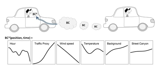
1. Introduction
2. Methodology
2.1. Experimental Design and Measurement Processing
2.2. Model Covariates
2.3. GAM Modeling and Auto-Correlation in Time Series Analysis
3. Data Exploration and Models
3.1. Summary Statistics and Lag Investigation
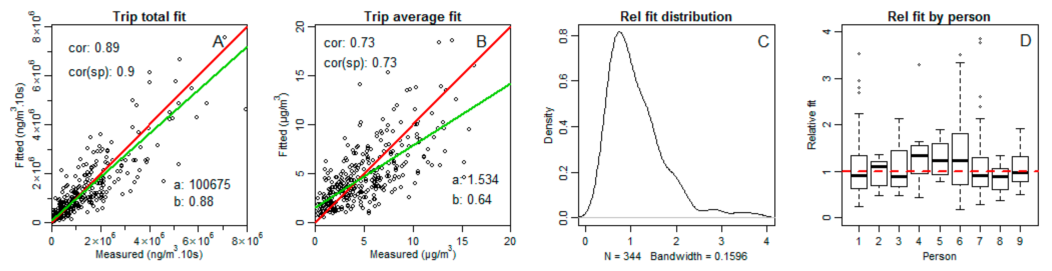
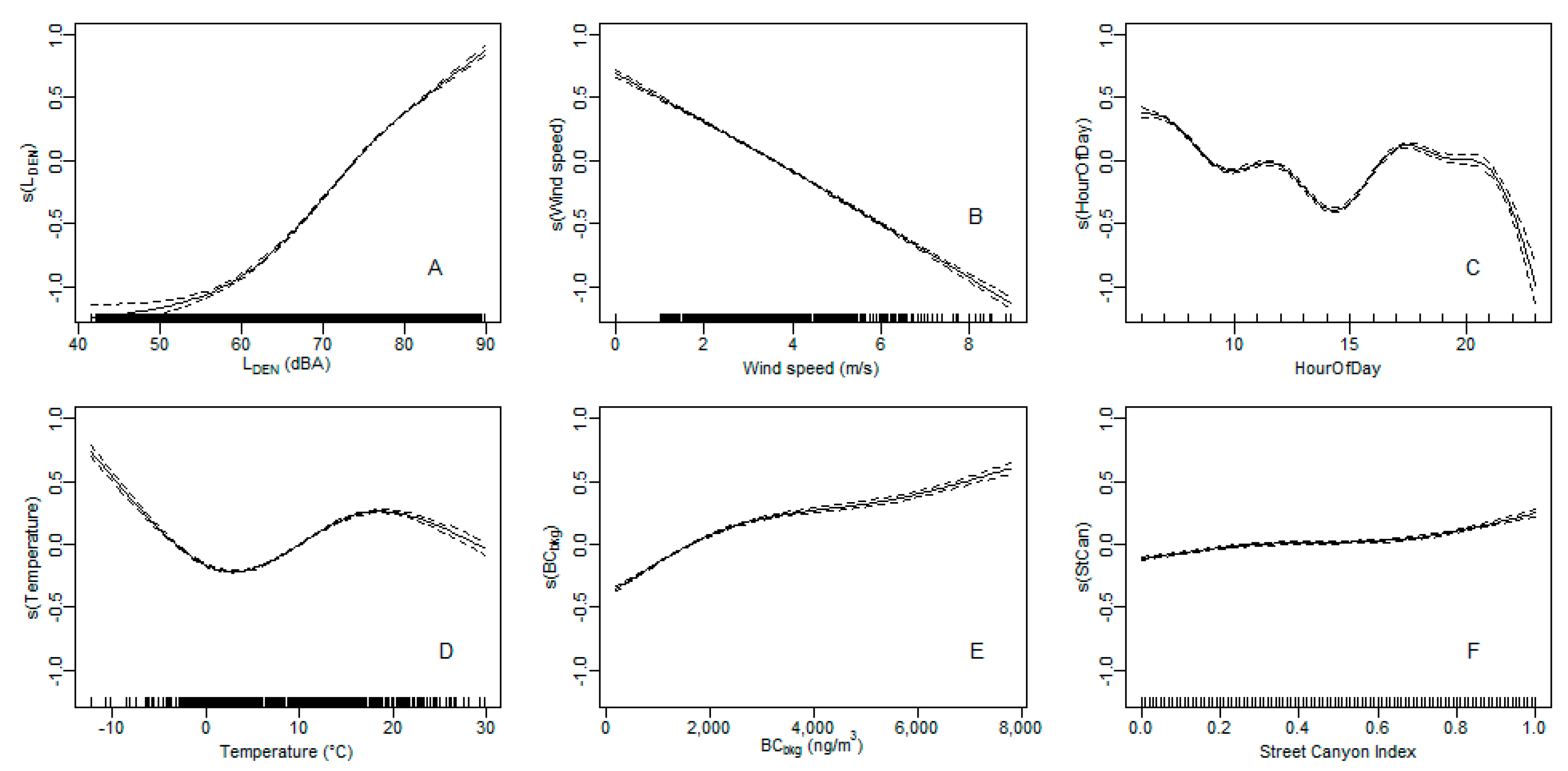
3.2. Non-Linear In-Vehicle Exposure Characteristics
3.3. Comparing Traffic-Related Data Sources
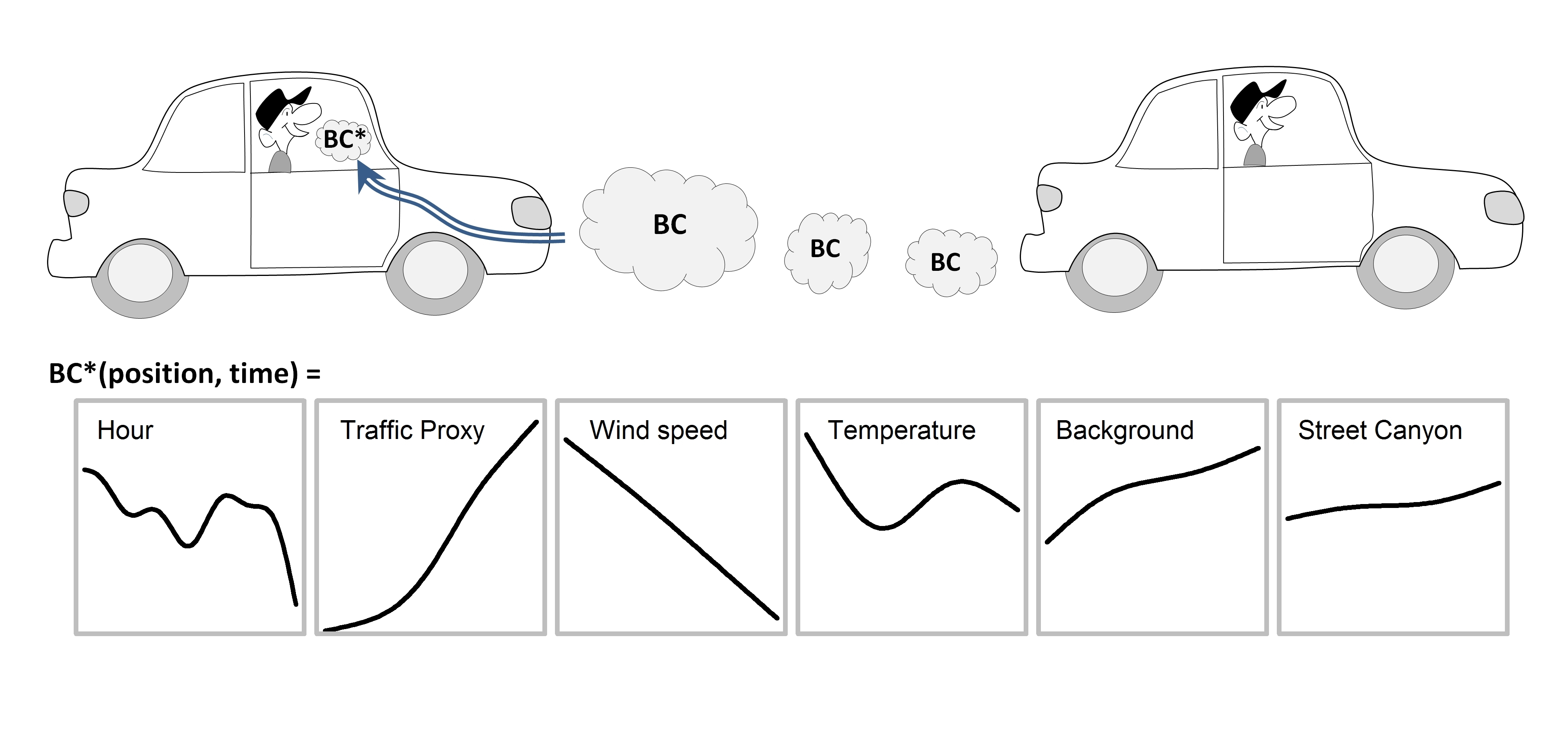
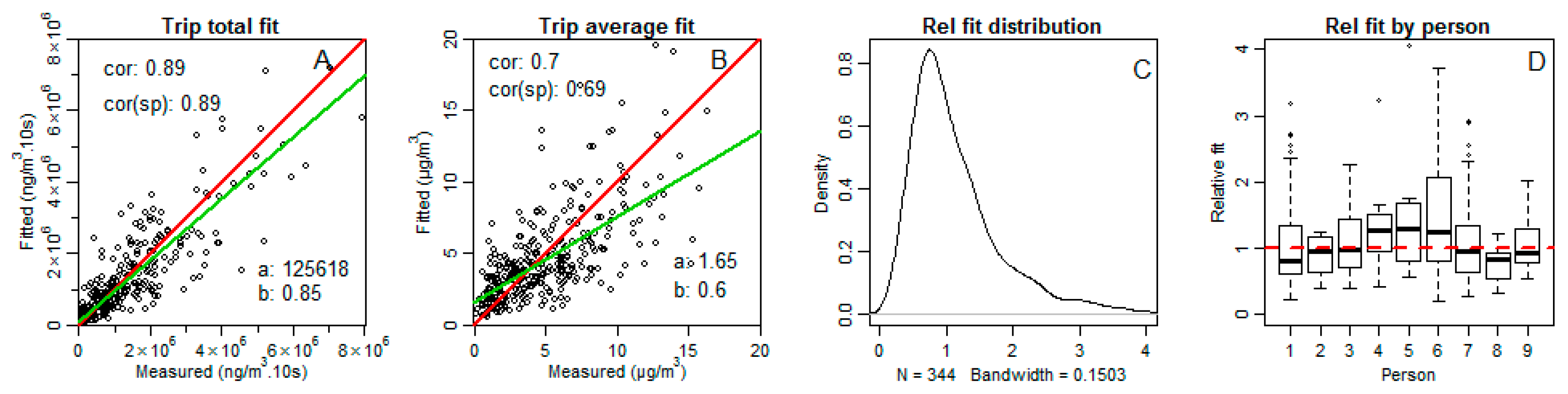
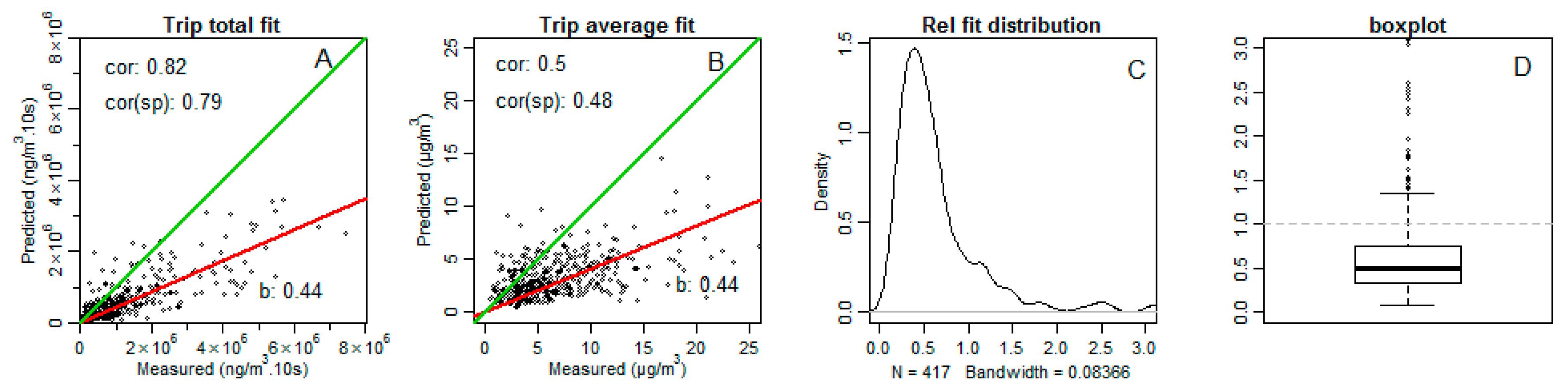
4. External Validation
4.1. Properties of the External Citizen Science Campaign
- Temporal resolution: 10 s for the µLUR model versus 5-min resolution for EXD
- Year of sampling: 2013 for µLUR, 2010–2011 for EXD
- Season: all year seasonally-balanced campaign for µLUR and an unbalanced combination of summer (six household) and a winter campaign (19 households) for EXD.
4.2. Validation Data Workflow
4.3. External Validation
4.4. Investigating the Discrepancy
5. Discussion
5.1. Translating the Complexity of In-Vehicle Exposure to Applications for Epidemiologists
5.2. Noise Maps as a Ubiquitous Traffic Data Source
5.3. Spatial Transferability of the Model
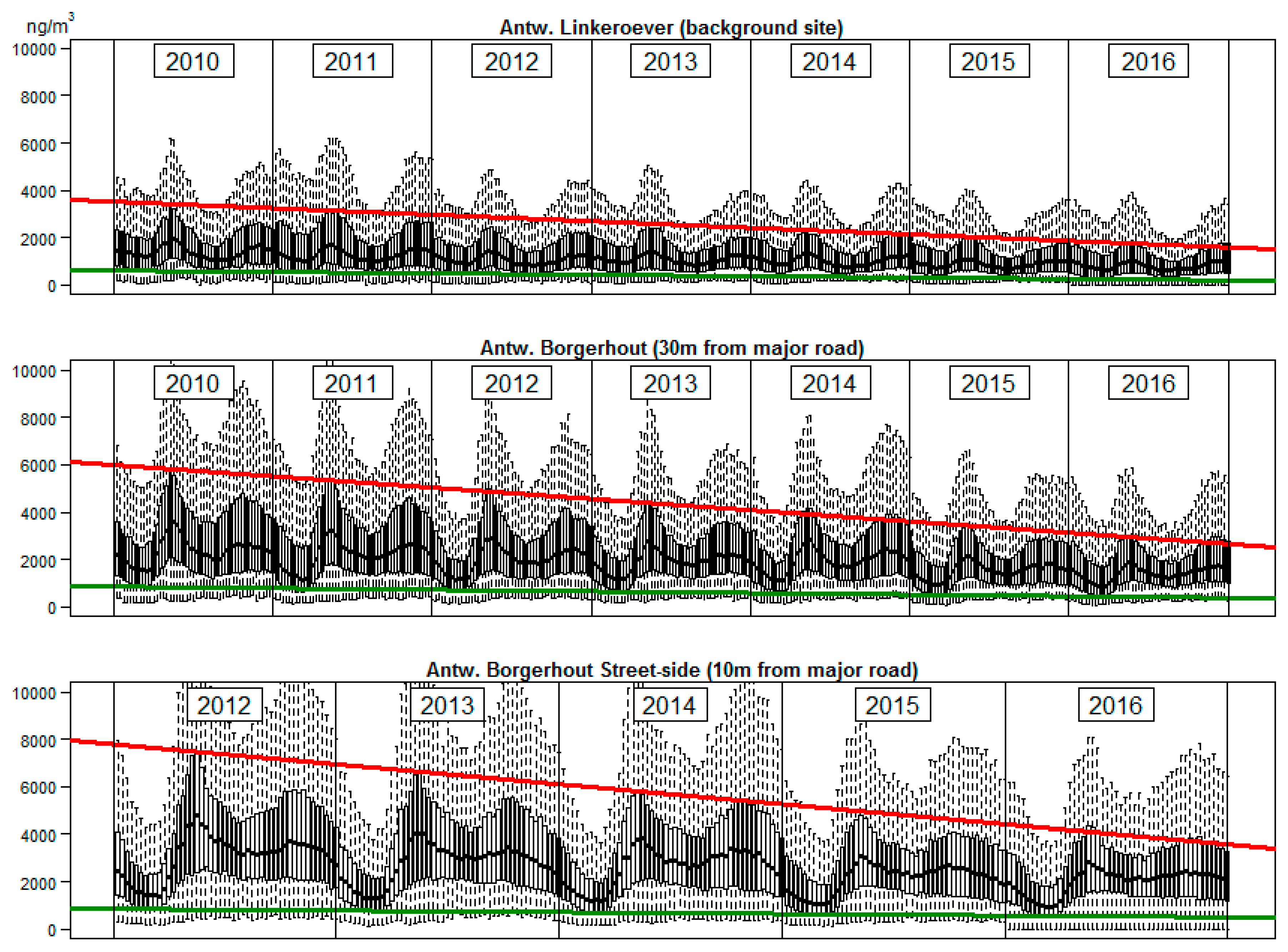
5.4. Changes in Particulate Emissions of the Vehicle Fleet
6. Conclusions
Supplementary Materials
Acknowledgments
Author Contributions
Conflicts of Interest
References
- WHO Europe. Health Effects of Black Carbon; WHO: Geneva, Switzerland, 2012; ISBN 978-92-890-0265-3. [Google Scholar]
- Dons, E.; Int Panis, L.; Van Poppel, M.; Theunis, J.; Willems, H.; Torfs, R.; Wets, G. Impact of time-activity patterns on personal exposure to black carbon. Atmos. Environ. 2011, 45, 3594–3602. [Google Scholar] [CrossRef]
- Dons, E.; Int Panis, L.; Van Poppel, M.; Theunis, J.; Wets, G. Personal exposure to black carbon in transport microenvironments. Atmos. Environ. 2012, 55, 392–398. [Google Scholar] [CrossRef]
- Karner, A.A.; Eisinger, D.S.; Niemeier, D.A. Near-Roadway Air Quality: Synthesizing the Findings from Real-World Data. Environ. Sci. Technol. 2010, 44, 5334–5344. [Google Scholar] [PubMed]
- Both, A.F.; Westerdahl, D.; Fruin, S.; Haryanto, B.; Marshall, J.D. Exposure to carbon monoxide, fine particle mass, and ultrafine particle number in Jakarta, Indonesia: Effect of commute mode. Sci. Total Environ. 2013, 443, 965–972. [Google Scholar] [CrossRef] [PubMed]
- Ioar, R.; Kumar, P.; Hagen-Zanker, A.; de Fatima Andrade, M.; Slovic, A.D.; Pritchard, J.P.; Geurs, K.T. Determinants of black carbon, particle mass and number concentrations in London transport microenvironments. Atmos. Environ. 2017, 161, 247–262. [Google Scholar]
- Williams, R.D.; Knibbs, L.D. Daily personal exposure to black carbon: A pilot study. Atmos. Environ. 2016, 132, 296–299. [Google Scholar] [CrossRef]
- Betancourt, R.M.; Galvis, B.; Balachandran, S.; Ramos-Bonilla, J.P.; Sarmiento, O.L.; Gallo-Murcia, S.M.; Contreras, Y. Exposure to fine particulate, black carbon, and particle number concentration in transportation microenvironments. Atmos. Environ. 2017, 157, 135–145. [Google Scholar] [CrossRef]
- Okokon, E.O.; Yli-Tuomi, T.; Turunen, A.W.; Taimisto, P.; Pennanen, A.; Vouitsis, I.; Samaras, Z.; Voogt, M.; Keuken, M.; Lanki, T. Particulates and noise exposure during bicycle, bus and car commuting: A study in three European cities. Environ. Res. 2017, 154, 181–189. [Google Scholar] [CrossRef] [PubMed]
- Kingham, S.; Longley, I.; Salmond, J.; Pattinson, W.; Shrestha, K. Variations in exposure to traffic pollution while travelling by different modes in a low density, less congested city. Environ. Pollut. 2013, 181, 211–218. [Google Scholar] [CrossRef] [PubMed]
- Qiu, Z.; Song, J.; Xu, X.; Luo, Y.; Zhao, R.; Zhou, W.; Xiang, B.; Hao, Y. Commuter exposure to particulate matter for different transportation modes in Xi’an, China. Atmos. Pollut. Res. 2017, 8, 940–948. [Google Scholar] [CrossRef]
- Dons, E.; Temmerman, P.; Van Poppel, M.; Bellemans, T.; Wets, G.; Int Panis, L. Street characteristics and traffic factors determining road users’ exposure to black carbon. Sci. Total Environ. 2013, 447, 72–79. [Google Scholar] [CrossRef] [PubMed]
- Dekoninck, L.; Botteldooren, D.; Int Panis, L. An instantaneous spatiotemporal model to predict a bicyclist’s black carbon exposure based on mobile noise measurements. Atmos. Environ. 2013, 79, 623–631. [Google Scholar] [CrossRef]
- Hudda, N.; Eckel, S.R.; Knibbs, L.D.; Sioutas, C.; Delfino, R.J.; Fruin, S.A. Linking in-vehicle ultrafine particle exposures to on-road concentrations. Atmos. Environ. 2012, 59, 578–586. [Google Scholar] [CrossRef] [PubMed]
- Knibbs, L.D.; de Dear, R.J.; Morawska, L. Effect of Cabin Ventilation Rate on Ultrafine Particle Exposure inside Automobiles. Environ. Sci. Technol. 2010, 44, 3546–3551. [Google Scholar] [CrossRef] [PubMed]
- Hudda, N.; Kostenidou, E.; Sioutas, C.; Delfino, R.J.; Fruin, S.A. Vehicle and Driving Characteristics That Influence In-Cabin Particle Number Concentrations. Environ. Sci. Technol. 2011, 45, 8691–8697. [Google Scholar] [CrossRef] [PubMed]
- Fruin, S.A.; Hudda, N.; Sioutas, C.; Defino, R.J. Predictive Model for Vehicle Air Exchange Rates Based on a Large, Representative Sample. Environ. Sci. Technol. 2011, 45, 3569–3575. [Google Scholar] [CrossRef] [PubMed]
- Lee, E.S.; Zhu, Y. Application of a High-Efficiency Cabin Air Filter for Simultaneous Mitigation of Ultrafine Particle and Carbon Dioxide Exposures inside Passenger Vehicles. Environ. Sci. Technol. 2014, 48, 2328–2335. [Google Scholar] [CrossRef] [PubMed]
- Ham, W.; Vijayan, A.; Schulte, N.; Herner, J.D. Commuter exposure to PM 2.5, BC, and UFP in six common transport microenvironments in Sacramento, California. Atmos. Environ. 2017, 167, 335–345. [Google Scholar] [CrossRef]
- Li, L.F.; Wu, J.; Hudda, N.; Sioutas, C.; Fruin, S.A.; Delfino, R.J. Modeling the Concentrations of On-Road Air Pollutants in Southern California. Environ. Sci. Technol. 2013, 47, 9291–9299. [Google Scholar] [CrossRef] [PubMed]
- Carslaw, D.C.; Beevers, S.D.; Tate, J.E. Modelling and assessing trends in traffic-related emissions using a generalised additive modelling approach. Atmos. Environ. 2007, 41, 5289–5299. [Google Scholar] [CrossRef]
- Patton, A.P.; Laumbach, R.; Ohman-Strickland, P.; Black, K.; Alimokhtari, S.; Lioy, P.J.; Kipen, H.M. Scripted drives: A robust protocol for generating exposures to traffic-related air pollution. Atmos. Environ. 2016, 143, 290–299. [Google Scholar] [CrossRef] [PubMed]
- Paas, B.; Stienen, J.; Vorländer, M.; Schneider, C. Modelling of Urban Near-Road Atmospheric PM Concentrations Using an Artificial Neural Network Approach with Acoustic Data Input. Environments 2017, 4, 26. [Google Scholar] [CrossRef]
- Lioy, P.J.; Smith, K.R. A discussion of exposure science in the 21st century: A vision and a strategy. Environ. Health Perspect. 2013, 121, 405. [Google Scholar] [CrossRef] [PubMed]
- Dekoninck, L.; Botteldooren, D.; Int Panis, L. Extending Participatory Sensing to Personal Exposure Using Microscopic Land Use Regression Models. Int. J. Environ. Res. Public Health 2017, 14, 586. [Google Scholar] [CrossRef] [PubMed]
- Hagler, G.S.W.; Yelverton, T.L.B.; Vedantham, R.; Hansen, A.D.A.; Turner, J.R. Post-processing method to reduce noise while preserving high time resolution in aethalometer real-time black carbon data. Aerosol Air Qual. Res. 2011, 11, 539–546. [Google Scholar] [CrossRef]
- Update of Noise Indicators (in Dutch) Actualisatie van de Geluidsindicatoren. Available online: http://www.milieurapport.be/Upload/main/0_onderzoeksrapporten/2014/verslag%20Geluidsindicatoren_MIRA_2013_final_TW-red.pdf (accessed on 20 Novemebr 2017).
- R Development Core Team. R: A Language and Environment for Statistical Computing; R Foundation for Statistical Computing: Vienna, Austria, 2008; ISBN 3-900051-07-0. Available online: http://www.R-project.org (accessed on 20 Novemebr 2017).
- Wood, S.N. On confidence intervals for generalized additive models based on penalized regression splines. Aust. N. Z. J. Stat. 2006, 48, 445–464. [Google Scholar] [CrossRef]
- Kohn, R.; Schimek, M.G.; Smith, M. Spline and kernel regression for dependent data. In Smoothing and Regression: Approaches, Computation, and Application; Wiley: Hoboken, NJ, USA, 2000; pp. 135–158. [Google Scholar]
- Peng, R.D.; Dominici, F.; Louis, T.A. Model choice in time series studies of air pollution and mortality. J. R. Stat. Soc. Ser. A Stat. Soc. 2006, 169, 179–203. [Google Scholar] [CrossRef]
- Bhaskaran, K.; Gasparrini, A.; Hajat, S.; Smeeth, L.; Armstrong, B. Time series regression studies in environmental epidemiology. Int. J. Epidemiol. 2013, 42, 1187–1195. [Google Scholar] [CrossRef] [PubMed]
- Dekoninck, L.; Botteldooren, D.; Panis, L.; Hankey, S.; Jain, G.; Karthik, S.; Marshall, J. Applicability of a noise-based model to estimate in-traffic exposure to black carbon and particle number concentrations in different cultures. Environ. Int. 2015, 74, 89–98. [Google Scholar] [CrossRef] [PubMed]
- Xu, B.; Liu, S.; Liu, J.; Zhu, Y. Effects of vehicle cabin filter efficiency on ultrafine particle concentration ratios measured in-cabin and on-roadway. Aerosol Sci. Technol. 2011, 45, 234–243. [Google Scholar] [CrossRef]
- Cai, J.; Yan, B.; Kinney, P.L.; Perzanowski, M.S.; Jung, K.; Li, T.; Xiu, G.; Zhang, D.; Olivo, C.; Ross, J.; et al. Optimization approaches to ameliorate humidity and vibration related issues using the MicroAeth black carbon monitor for personal exposure measurement. Aerosol Sci. Technol. 2013, 47, 1196–1204. [Google Scholar] [CrossRef] [PubMed]
- Dons, E.; Van Poppel, M.; Int Panis, L.; De Prins, S.; Berghmans, P.; Koppen, G.; Matheeussen, C. Land use regression models as a tool for short, medium and long term exposure to traffic related air pollution. Sci. Total Environ. 2014, 476, 378–386. [Google Scholar] [CrossRef] [PubMed]
- Khoury, M.J.; Lam, T.K.; Ioannidis, J.P.A.; Hartge, P.; Spitz, M.R.; Buring, J.E.; Chanock, S.J.; Croyle, R.T.; Goddard, K.A.; Ginsburg, G.S.; et al. Transforming epidemiology for 21st century medicine and public health. Cancer Epidemiol. Biomark. Prev. 2013, 22, 508–516. [Google Scholar] [CrossRef] [PubMed]
- Reis, S.; Morris, G.; Fleming, L.E.; Beck, S.; Taylor, T.; White, M.; Depledge, M.H.; Steinle, S.; Sabel, C.E.; Cowie, H.; et al. Integrating health and environmental impact analysis. Public Health 2015, 129, 1383–1389. [Google Scholar] [CrossRef] [PubMed]
- Dekoninck, L.; Botteldooren, D.; Int Panis, L. Using city-wide mobile noise assessments to estimate annual exposure to Black Carbon. Environ. Int. 2015, 83, 192–201. [Google Scholar] [CrossRef] [PubMed]
- Hoek, G.; Beelen, R.; de Hoogh, K.; Vienneau, D.; Gulliver, J.; Fischer, P.; Briggs, D. A review of land-use regression models to assess spatial variation of outdoor air pollution. Atmos. Environ. 2008, 42, 7561–7578. [Google Scholar] [CrossRef]
- Beelen, R.; Hoek, G.; Vienneau, D.; Eeftens, M.; Dimakopoulou, K.; Pedeli, X.; Tsai, M.-Y.; Künzli, N.; Schikowski, T.; Marcon, A.; et al. Development of NO2 and NOx land use regression models for estimating air pollution exposure in 36 study areas in Europe—The ESCAPE project. Atmos. Environ. 2013, 72, 10–23. [Google Scholar] [CrossRef]
- Patton, A.P.; Zamore, W.; Naumova, E.N.; Levy, J.I.; Brugge, D.; Durant, J.L. Transferability and generalizability of regression models of ultrafine particles in urban neighborhoods in the Boston area. Environ. Sci. Technol. 2015, 49, 6051–6060. [Google Scholar] [CrossRef] [PubMed]
- EU Commision. The Environmental Noise Directive (2002/49/EC). Available online: http://ec.europa.eu/environment/noise/directive_en.htm (accessed on 18 Novemebr 2017).
- Cames, M.; Helmers, E. Critical evaluation of the European diesel car boom-global comparison, environmental effects and various national strategies. Environ. Sci. Eur. 2013, 25, 15. [Google Scholar] [CrossRef]


| External data | Description |
|---|---|
| Speed and acceleration | The speed and acceleration were calculated based on the sequence of positions resulting from the GPS data (on a 10-s basis for speed and the next position for the acceleration). |
| Relative speed | The speed limit of the road was retrieved from the traffic database. Relative speed was calculated as actual speed divided by the speed limit. |
| Meteorology | Weather data are available at a temporal resolution of 30 min from nine official measurement stations of the RMI (Royal Meteorological Institute, Belgium). |
| Traffic counts (hourly) | Measurement hour and actual road segment back to the traffic database (weekdays only). Heavy vehicles count as 2 (standard approach by the mobility experts in Flanders). This factor is based on traffic evaluations and is not related to noise or PM emissions. |
| Traffic counts (AAWT) | Annual average weighted traffic: Sum all traffic for the road (sum of hourly data). |
| LDEN noise mapping | The underlying traffic data are routed on the physical network by using the open source network functionality (networkX). This approach improves the pre-existing approach to calculate the exposure model based on the generalized network (with straight connections in between the crossroads) (see Figure S3b). The underlying emission points of the noise map are calculated on smooth buffers around the road segments to avoid jitter due to changing distances to the road segment polylines (10-, 20-, 50- and 100-m buffers combined with a 100 × 100 point grid at larger distances from the road network. The map-matched GPS data points from the vehicle traps are evaluated on a 20-m interpolated grid. |
| Lday,hour noise map | Hourly variant of the Lday noise map by applying a fixed diurnal correction based on the average diurnal pattern for the traffic dataset over a full year (working days only). |
| PM10 map | GPS point is mapped to the PM10 grid of spatial resolution 100 m from a 1-km grid air pollution calculation model (2011). The spatial resolution of this map does not express the impact of local features (major roads and highways). |
| Street canyon index | Finds the closest street canyon evaluation (evaluated every 50 m along the network in Flanders and Brussels). |
| Black carbon background concentrations | Measurement location Antwerpen-Linkeroever (40AL01): black carbon concentrations in µg/m3 for a 30-min resolution, available from 2010 till the present. |
| F-Values of Covariates | ||||||||||||||||
|---|---|---|---|---|---|---|---|---|---|---|---|---|---|---|---|---|
| Intercept (ng/m3) | Wind Speed | Temperature | Humidity | BC bkg | Traffic Count by Hour | LDEN | Hour of Day | Speed (Rel Speed Limit) | Speed | Acceleration | PM10 | Street Canyon | # Samples | Dev. expl. | AIC | |
| Investigating Lag and Weight | ||||||||||||||||
| BC_LAG0 | 3479 | 1360 | 621 | 129 | 1059 | 718 | 856 | 128 | 280 | 187 | 34 * | 14 * | 90 | 77,960 | 36.9% | 195,899 |
| BC_LAG60 | 3685 | 1427 | 924 | 154 | 1281 | 808 | 1090 | 142 | 257 | 198 | 41 | 13 * | 192 | 79,158 | 39.1% | 188,584 |
| BC_LAG120 | 3592 | 1535 | 778 | 135 | 1159 | 817 | 1019 | 141 | 275 | 142 | 46 | 16 * | 147 | 79,158 | 38.9% | 190,696 |
| BC_LAG60_WBC | 4029 | 1938 | 1023 | 240 | 957 | 845 | 1171 | 241 | 360 | 195 | 61 | 43 | 175 | 79,158 | 46.9% | 252,213 |
| F-Values of Covariates | ||||||||||||||
|---|---|---|---|---|---|---|---|---|---|---|---|---|---|---|
| Intercept (ng/m3) | Wind Speed | Temprature | BCbkg | StCan | Speed (rel) | Accel | Hour of Day | Traffic (Hour) † | Traffic (AAWT) | LDEN | Lday † | Deviance Explained | AIC | |
| Investigating Traffic Covariates (Including Traffic Dynamics) | ||||||||||||||
| BC_LDAYWH† | 4056 | 2869 | 843 | 879 | 318 | 497 | 28 | 587 | 3429 | 44.0% | 256,387 | |||
| BC_LDENWH | 4058 | 2666 | 862 | 882 | 117 | 475 | 27 | 314 | 3364 | 44.0% | 256,393 | |||
| BC_TRAFWAADTH | 4061 | 2145 | 833 | 971 | 81 | 567 | 67 | 284 | 3241 | 43.7% | 256,759 | |||
| BC_TRAFWH† | 4056 | 2151 | 825 | 950 | 71 | 571 | 65 | 282 | 3037 | 43.3% | 257,301 | |||
| BC_LDENW | 4076 | 2616 | 764 | 1250 | 151 | 521 | 24 | 3382 | 42.2% | 258,859 | ||||
| BC_TRAFWAADT | 4077 | 2496 | 735 | 1311 | 73 | 637 | 66 | 3305 | 42.1% | 258,994 | ||||
| BC_TRAFW† | 4072 | 2649 | 677 | 1274 | 62 | 654 | 65 | 3108 | 41.7% | 259,521 | ||||
| BC_LDAYW† | 4091 | 2654 | 672 | 1323 | 21 * | 564 | 25 | 2611 | 40.7% | 260,928 | ||||
| Investigating Traffic Covariates (Without Traffic Dynamics) | ||||||||||||||
| BCR_LDENWH | 4081 | 2627 | 852 | 769 | 151 | 346 | 3858 | 42.2% | 258,916 | |||||
| BCR_LDAYWH† | 4081 | 2636 | 830 | 762 | 152 | 634 | 3806 | 42.1% | 259,031 | |||||
| BCR_TRAFWAADTH | 4092 | 2322 | 769 | 839 | 116 | 336 | 3408 | 41.3% | 260,132 | |||||
| BCR_TRAFWH† | 4087 | 2338 | 754 | 819 | 114 | 342 | 3200 | 40.9% | 260,686 | |||||
| BCR_LDENW | 4103 | 2794 | 749 | 1144 | 148 | 3852 | 40.1% | 261,631 | ||||||
| BCR_TRAFWAADT | 4114 | 2721 | 662 | 1191 | 123 | 3435 | 39.3% | 262,765 | ||||||
| BCR_TRAFW† | 4109 | 2867 | 601 | 1156 | 114 | 3207 | 38.8% | 263,370 | ||||||
| BCR_LDAYW† | 4122 | 2876 | 651 | 1218 | 50 | 3000 | 38.4% | 263,932 | ||||||
© 2017 by the authors. Licensee MDPI, Basel, Switzerland. This article is an open access article distributed under the terms and conditions of the Creative Commons Attribution (CC BY) license (http://creativecommons.org/licenses/by/4.0/).
Share and Cite
Dekoninck, L.; Int Panis, L. A High Resolution Spatiotemporal Model for In-Vehicle Black Carbon Exposure: Quantifying the In-Vehicle Exposure Reduction Due to the Euro 5 Particulate Matter Standard Legislation. Atmosphere 2017, 8, 230. https://doi.org/10.3390/atmos8110230
Dekoninck L, Int Panis L. A High Resolution Spatiotemporal Model for In-Vehicle Black Carbon Exposure: Quantifying the In-Vehicle Exposure Reduction Due to the Euro 5 Particulate Matter Standard Legislation. Atmosphere. 2017; 8(11):230. https://doi.org/10.3390/atmos8110230
Chicago/Turabian StyleDekoninck, Luc, and Luc Int Panis. 2017. "A High Resolution Spatiotemporal Model for In-Vehicle Black Carbon Exposure: Quantifying the In-Vehicle Exposure Reduction Due to the Euro 5 Particulate Matter Standard Legislation" Atmosphere 8, no. 11: 230. https://doi.org/10.3390/atmos8110230
APA StyleDekoninck, L., & Int Panis, L. (2017). A High Resolution Spatiotemporal Model for In-Vehicle Black Carbon Exposure: Quantifying the In-Vehicle Exposure Reduction Due to the Euro 5 Particulate Matter Standard Legislation. Atmosphere, 8(11), 230. https://doi.org/10.3390/atmos8110230