Abstract
Several types of non-precipitation echoes appear in radar images and disrupt the weather forecasting process. An anomalous propagation echo is an unwanted observation result similar to a precipitation echo. It occurs through radar-beam ducting because of the temperature, humidity distribution, and other complicated atmospheric conditions. Anomalous propagation echoes should be removed because they make weather forecasting difficult. In this paper, we suggest an ensemble classification method based on an artificial neural network and a clustering-based subset-selection method. This method allows us to implement an efficient classification method when a feature space has complicated distributions. By separating the input data into atomic and non-atomic clusters, each derived cluster will receive its own base classifier. In the experiments, we compared our method with a standalone artificial neural network classifier. The suggested ensemble classifier showed 84.14% performance, which was about 2% higher than that of the k-means clustering-based ensemble classifier and about 4% higher than the standalone artificial neural network classifier.
1. Introduction
Weather forecasting uses information obtained by observing and analyzing atmospheric phenomena. Through developments in science and technology, it is possible to analyze atmospheric conditions using radar, satellite, or other advanced devices. Radar, especially, provides valuable information in the weather prediction process because of its fine resolution in the space domain [1], real-time observations, wide and remote observation area, etc. Therefore, it is essential to analyze radar data precisely and accurately. However, some types of unwanted radar echoes are included in the radar data. They are called non-precipitation echoes.
A quality control process [2] is implemented in many practical fields. However, the quality-control process tends to depend on an expert’s opinion. In other words, subjective and inconsistent decisions are possibly derived. These decisions can decrease the reliability of the weather forecasting result. To overcome these drawbacks, previous studies have investigated automated quality-control processes or decision-support systems to assist the experts [3].
Representative non-precipitation echoes include chaff, sea clutter, anomalous propagation, etc. Particularly, anomalous propagation echoes can have a significant effect on the quantitative precipitation estimation process. It occurs in certain nonstandard refraction conditions in the atmosphere where the radar beam is bent unusually. Radar-beam ducting makes radar-data analysis more complicated because anomalous propagation surface echo can be misinterpreted as heavy precipitation [4]. For many years, researchers have studied the detection of anomalous propagation echoes from radar data. The techniques can be classified as follows: fuzzy logic techniques [5,6,7]; artificial neural networks [8,9,10]; Bayesian classifiers [11]; case studies [12]; statistical approaches [13]; etc.
In this paper, we suggest an ensemble classification method [14]. The main concept of ensemble classification is to obtain a single classifier, which is more accurate and reliable, by combining a set of base classifiers. When the input space is complex and not linearly separable, this approach can improve the performance. We chose an artificial neural network as the base classifier [15]. Furthermore, we applied a clustering-based subset-selection method for training the base classifiers. According to the previous approach described in [14], we selected k-means clustering for separating the input space into atomic or non-atomic clusters. However, k-means clustering is extremely sensitive to the selected number of clusters (k). Therefore, we changed the clustering method to the Chinese restaurant process (CRP) [16], which is discussed in Section 3.1.2.
The rest of the paper is organized as follows. Section 2 elucidates the anomalous propagation echo. Section 3 explains the ensemble classification method, including the clustering-based subset-selection method, the artificial neural network as a base classifier, and an overview of the suggested system. After that, experimental results with actual radar observation data are described in Section 4. Finally, our conclusions and future work are presented in Section 5.
2. Anomalous Propagation Echo
Radar has a different observation efficiency compared to other remote-sensing devices because it uses the radar-beam propagation path, which is significantly influenced by atmospheric conditions. The propagation path can be changed by multiple factors, e.g., temperature, pressure, water vapor in the air, etc. The paths are classified into subrefraction, standard refraction, superrefraction, and ducting [17], as shown in Figure 1a.
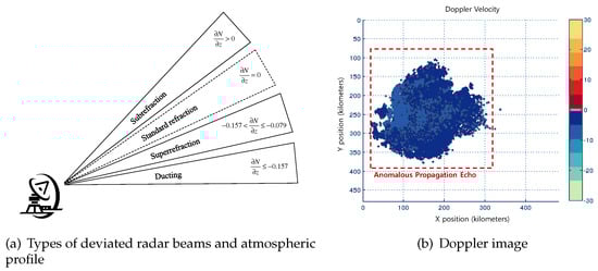
Figure 1.
Anomalous propagation echo.
In [18], the four modes of the radar-beam propagation path are distinguished by an approximated equation for the vertical gradient of refractivity, as shown in Equation (1).
where ρ is the curvature radius, N is the refractivity, and z is the vertical coordinate. For standard refraction, has a range between 0 and m. Subrefraction, which has , indicates that the radar-beam propagation path is refracted away from the ground surface more than in standard refraction. As a result, a subrefracting radar underestimates the altitude of the target. However, for superrefraction, whose is between and m, the radar-beam propagation path is refracted toward the ground surface more than usual. Consequently, a superrefracting radar overestimates the altitude of the target. Moreover, ducting is caused by a severely refracted radar-beam propagation path, < m. When ducting occurs, the beam is trapped between a certain atmospheric layer and the ground.
When the radar-beam path follows a standard refraction, the meteorological observations are accurate. However, it is possible to obtain a severely erroneous observation by recognizing surface objects as reflectors in the atmosphere if ducting occurs. When ducting occurs, a strong radar echo is observed by the surface scattering of the radar-beam path. This is called an anomalous propagation echo, and it causes problems when radar data is used in the quantitative precipitation estimation process. Furthermore, an anomalous propagation echo may be identified as a precipitation echo unless a proficient expert is involved in the forecasting process. Therefore, it is essential to remove anomalous propagation echoes for accurate weather prediction. In practical weather forecasting, experts selectively use several complicated rules to remove anomalous propagation echoes from the radar data [19]. The representative experts’ rules are presented below.
- The echo has a small Doppler velocity (≈0 m/s).
- The echo has slightly different characteristics on the ground or on the sea surface.
- The maximum altitude of the echo is low.
- The reflectivity of the echo is distributed discontinuously in the vertical and horizontal directions.
The above expert’s rules indicate that the Doppler velocity and reflectivity are essential information for anomalous propagation echo detection. Furthermore, it is important to identify the surface where the anomalous propagation echo occurs as mentioned in Rule 2. The echo consists of two types: ground clutter and sea clutter. Ground clutter has a Doppler velocity closer to zero than sea clutter. However, the fact is evident that the anomalous propagation echo has a near-zero Doppler velocity as mentioned in Rule 1. Figure 1b shows an example of the sea clutter. It confirms that the anomalous propagation echo has a small Doppler velocity.
3. Ensemble Classification
In recent years, many algorithms have been proposed for classification. However, conventional classifiers are generally based on a single classifier or a simple combination of classifiers, and show relatively moderate performance. Unfortunately, even exquisitely designed classifiers have deficiencies, which means that they cannot appropriately separate the samples. Therefore, many researchers have recently studied ensemble classifiers. A variety of classifiers, either different types of classifiers or different instances of the same classifier, are combined before a final classification decision is made. The objective of an ensemble classifier using the clustering-based subset-selection method is to diversify by explicitly partitioning the input data set into multiple clusters, and engaging a set of base classifiers to learn the decision boundaries within the cluster patterns.
The rest of this section proceeds as follows. First, the subset-selection method based on clustering is explained. Second, a brief description of the artificial neural network chosen as a base classifier is given. Finally, we elucidate the operating principles of the suggested method.
3.1. Clustering-Based Subset-Selection Method
Clustering involves grouping the given data based on similarities; a cluster is a group of finite patterns. Clustering can be divided into two approaches, hierarchical and nonhierarchical. Hierarchical clustering makes a tree-like structure from the given data by grouping it over a variety of scales. It consists of two approaches, agglomerative (bottom-up) and divisive (top-down). Nonhierarchical clustering forms clusters using successive merging or splitting, regardless of the hierarchy structure.
3.1.1. k-Means Clustering
k-means clustering is a well-known nonhierarchical clustering method. The operating principles of k-means clustering are as follows. First, set the number of clusters, k, which allows the method to divide the entire data into k pieces. Second, randomly choose k amount of data to set the initial centroid of each cluster. Third, update the centroid by continuously calculating the distance from the centroid to the given data until the stopping criterion is satisfied. The methods for deriving the distance between the given data and the centroid are the Euclidean method, Mahalanobis method, etc. Equation (2) shows an objective function for k-means clustering:
where stands for the input data points and is the centroid coordinates of the j-th cluster.
Generally, the nonhierarchical approach is processed with a strong assumption of how many clusters will be generated. In other words, k-means clustering is extremely sensitive to the selected number of clusters, k. The k parameter is determined heuristically and determines the number of base classifiers. Therefore, it is essential to set an appropriate k parameter. If k is too small, it may not differentiate between a single classifier and an ensemble classifier because the number of base classifiers is too small. However, if k is too large, the derived cluster may consist of a small amount of data.
3.1.2. Chinese Restaurant Process
Considering the aforementioned problems, we changed the clustering method to the CRP (Chinese Restaurant Process), which is a nonhierarchical method and closely related to DPGMM (Dirichlet Process Gaussian Mixture Model). One of the advantages of the CRP is that we do not need to set parameter k in advance, which decides how many clusters will be generated using the data. Customers indicate given data points. Tables indicate clusters. Specific customers who sit at the same table indicate specific data points that belong to the same cluster. A sequence of customers sits down at the tables of a Chinese restaurant. A newly arrived customer can sit at an occupied table with a probability proportional to the number of customers at the table, or at an empty table with a probability proportional to a concentration parameter. In summary, the CRP is a distribution over partitions that embodies the assumed prior distribution over cluster structures [16].
Let denote the table assignment of the i-th customer as shown in Equation (3); assume that customers occupy N tables, and let denote the number of customers sitting at table n:
where α is a given concentration parameter. When all N tables are occupied by C customers, their table assignments result in a random partition. Since the number of occupied tables is random, the CRP can provide a flexible model in which the number of clusters is determined by the data.
3.2. Artificial Neural Network
An artificial neural network is a popular computational model formed from hundreds of artificial neurons connected with weights. An artificial neural network has many advantages: it detects complex nonlinear relationships between independent and dependent variables, it can be developed using multiple different training algorithms, and it requires relatively less training data to implement. In this study, we apply an artificial neural network as a base classifier for the ensemble classification method. To divide the input space into subsets using a clustering method, the structure of the artificial neural network should be simple. Therefore, we chose an artificial neural network with ten neurons in one hidden layer.
3.3. Overview of Suggested System
Figure 2 shows how the proposed system works. Before explaining how the system works, it is necessary to point out what kinds of observation results are available and which ones the proposed system selects. There are several types of observation results in the raw radar data: corrected reflectivity (CZ), Doppler velocity (VR), uncorrected reflectivity (DZ) and spectrum width (SW), as shown in Figure 2. We chose CZ and VR for classification using the rules mentioned above. The difference between CZ and DZ is that the former have been noise-filtered and the latter have not been noise-filtered.
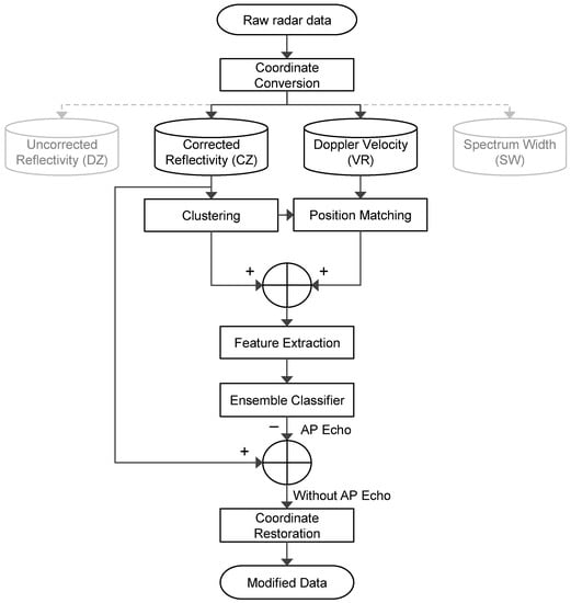
Figure 2.
System overview of the proposed method.
At the first step, coordinate conversion is performed using the TRMM (Tropical Rainfall Measuring Mission) Radar Software Library [20] for reading and analyzing UF (universal format) radar data. We convert the data using the library into CAPPI (constant altitude plan position indicator) along the altitude. After that, we assign x, y and z to each data point: x- and y-axes at z-altitude. The purpose of converting the coordinate is for the convenience of applying a hierarchical clustering in the next step. We needed to consider the cosine and root operator for obtaining distance in polar coordinate. However, when we convert the coordinate into the Euclidean coordinate, it is possible to get the distance without using the cosine function: . Moreover, if we considered adjacent data points only on horizontal, vertical, and diagonal positions, we can obtain the distance without root operator: . The decreased computational complexity might help to improve the performance of the proposed system. Secondly, the hierarchical clustering algorithm [21] is applied to categorize the radar data. We put the corrected reflectivity data as a reference since the quantitative precipitation estimation is closely related to reflectivity. Therefore, the hierarchical clustering is applied to the corrected reflectivity data, and corresponding Doppler velocity data is selected in the position matching process. Thirdly, a feature extraction process derives input data for classification. The proposed classifier carries out an identification process of anomalous propagation echoes by using the given inputs. The identified anomalous propagation echo is removed in the corrected reflectivity data after the classification process. At last, the coordinate restoration process is performed to maintain the consistency of the data storage.
Table 1 shows a part of the dataset. The reflectivity and the Doppler velocity are used as inputs according to the aforementioned experts’ rules. In addition, average and maximum values are selected through the feature extraction process. One more input is a cluster size that indicates the number of points of clusters categorized by the hierarchical clustering. The reason why the cluster size is chosen as one of classification inputs is for considering the size of interest. We assume that influences of the anomalous propagation echo are negligible if the size is not big enough. We select 15-day discontinuous radar data from April to May, which contains the anomalous propagation echo events. From the data, we can get approximately 3500 clusters for making the learning data, and values of the cluster size tend to be more than 200. Based on the tendency, we consider the value as a classification input.

Table 1.
Dataset for classification.
The classification inputs are selected as the maximum and mean reflectivity, mean Doppler velocity, and cluster size. We choose the reflectivity and Doppler velocity for reasons described in Section 2, and, because, according to case studies, their influence is significant when the anomalous propagation echo is relatively large. Each property is derived as shown in Equations (4)–(6), respectively, where is the cluster ID; is the data index of the cluster; and x, y, and z stand for the cluster coordinates in Cartesian coordinate 3D volume data. The cluster size is derived by n, which is obtained in the clustering process:
Our suggested ensemble classification method is shown in Figure 3 and Figure 4. Figure 3 shows the process of the ensemble classifier. Figure 4 shows the process of applying the ensemble classifier using test data.
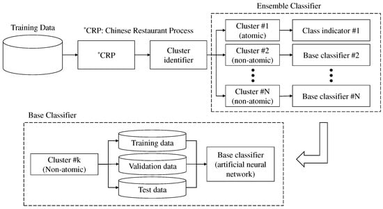
Figure 3.
The suggested ensemble classification algorithm—construct ensemble classifier.
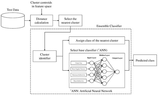
Figure 4.
The suggested ensemble classification algorithm—apply to test data.
The process for implementing the ensemble classifier using training data is as follows. First, the CRP is applied to the training data. After clustering, the clusters are examined by a cluster identifier that can separate the clusters into atomic and non-atomic types. In this context, an atomic type means that all the data in the cluster have the same class, and a non-atomic type means that the data in the cluster has more than one class.
If the cluster is atomic, the cluster indicator is chosen as a base classifier, which derives its output from the cluster’s class. For example, let’s consider the following three conditions: test data is given, the closest cluster of the given test data is atomic, and a class of the closest cluster is 1. In this case, the cluster indicator assigns class 1 to the given test data.
If the cluster is non-atomic, the artificial neural network is chosen as a base classifier. To train the artificial neural network as a base classifier, the data of the selected cluster were divided into training, validation, and test data. The validation data is used to minimize over-fitting. Over-fitting is a modeling error that occurs when a function is too closely fit to a limited set of data points. In other words, accuracy over training data increases when accuracy over unseen data stays the same or decreases. To prevent the over-fitting, validation data is essential. In this study, we chose the ratio of each data set as 6:2:2 for implementing the base classifier.
The process for applying the implemented ensemble classifier using test data is as follows. First, the Euclidean distance is determined between the test data and the centroid coordinates, which were derived using the CRP using Equation (7):
The cluster with the smallest Euclidean distance is chosen as the nearest cluster. After that, the test data and the selected nearest cluster are used as inputs to the ensemble classifier. The type of the nearest cluster is determined using the cluster identifier. If the nearest cluster is atomic, the predicted class is assigned the class of the selected cluster. If the nearest cluster is non-atomic, the predicted class is assigned by the artificial neural network result, which belongs to the selected cluster, using the test data.
4. Results and Discussion
We selected actual appearance cases to verify the proposed system. The following process generated the learning dataset: at first, we gathered the radar data including the anomalous propagation echo. After that, the hierarchical clustering was applied to make the training dataset. The clusters categorized either anomalous propagation or others using experts’ weather forecasting results. The results were given in images that included the experts’ decision of the echoes. For example, in a radar site, the left-upper region indicated anomalous propagation echoes, and the lower part meant heavy precipitation. We considered the images as ground truth in this paper.
We applied a confusion matrix to verify the accuracy, as shown in Equation (8). In this equation, stands for true positive, for true negative, for false positive and for false negative. The true parameter indicates an anomalous propagation echo, and the false parameter stands for a non-anomalous propagation echo. By considering the positive results in Equation (8), the performance of the experimental results could be derived:
Furthermore, to compare the previous approach [14] that used k-means clustering, it is essential to validate the implemented ensemble classifier over several trials. Therefore, this study derived the averages and standard deviations of the deployed ensemble classifier using five tests with randomly chosen input datasets. For comparison, an artificial neural network with a structure of 10 neurons in one hidden layer was also implemented. Moreover, we selected 5 and 10 for the k parameters.
Experimental results using the CRP and k-means clustering are shown in Figure 5. In Figure 5, circle marks indicate anomalous propagation echo, and cross marks indicate others. Figure 5a–c describe the clustering results distinguished by colors. The derived cluster number of the CRP was 7. It is confirmed that the CRP method categorized the feature evenly compared to k-means clustering as shown in Figure 5. In other words, the k-means clustering failed to generate appropriate subsets because the different clusters were concentrated in the left-upper area. Therefore, the k-means clustering-based subset selection method could make almost no difference for using the entire feature space.
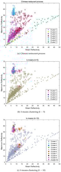
Figure 5.
Comparison of the Chinese restaurant process and k-means clustering (o: AP, x: others).
Table 2 shows the experimental results comparing the ensemble classifiers. For estimating how accurately a predictive model will perform in practice, 5-fold cross-validation is used in the experiments. According to Table 2, the average performance of the CRP-based ensemble classifier is 84.14% with 0.61 standard deviations, while those of the k-means clustering-based methods are 82.18% and 82.13% with standard deviations of 1.25 and 1.44, respectively. Moreover, the average performance of the standalone artificial neural network is 80.86% with 0.87 standard deviations. The result confirmed that the CRP-based ensemble classifier shows relatively better and more stable results than the k-means clustering-based classifier and the standalone artificial neural network classifier:
Table 2.
Experimental results of ensemble classifiers based on subset selection methods.
Furthermore, we applied a critical success index (CSI) [22] and a Heidke skill score (HSS) [23], as shown in Equations (9) and (10), to compare the performances of existing quality control methods. The performances of our proposed method are as follows: 0.764 for CSI and 0.706 for HSS. According to [10], HSS is 0.7 for clean atmosphere and 0.4 for the anomalous propagation events. In [24], the HSS is 0.8. In addition, in [6], CSI is 0.78. The performance of our proposed method shows similar to or better than the previous studies’ results compared to the existing methods. We can draw this conclusion from the fact that most of the previous research validated performance pixel-wise and in some studies used dual-polarimetric radar data. On the other hand, we verified the performance of our proposed method cluster-wise and used single-polarization radar data.
Figure 6, Figure 7 and Figure 8 show three of the experimental results using the ensemble classifier. As shown in Figure 6a, the left-lower side is an anomalous propagation echo on the sea surface, and the right-upper side is a precipitation echo. Figure 7a, almost the entire area, is represented as an anomalous propagation echo on the sea surface. In Figure 8a, the left-lower side is an anomalous propagation echo on the sea surface and the others are precipitation echoes. Figure 6b, Figure 7b and Figure 8b describe the anomalous propagation echo, which is separated by the suggested ensemble classifier. Finally, Figure 6c, Figure 7b and Figure 8c show the radar image without the separated anomalous propagation echo. Some small areas remain, and it seems that the anomalous propagation echo is hard to classify because we are not considering the small size clusters, and the characteristics might be similar to those of precipitation echoes. Consequently, it is confirmed that the suggested ensemble classifier can separate and remove the anomalous propagation echo successfully.
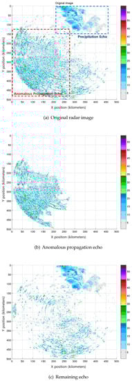
Figure 6.
Experimental results: Case 1.
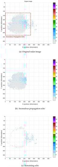
Figure 7.
Experimental results: Case 2.
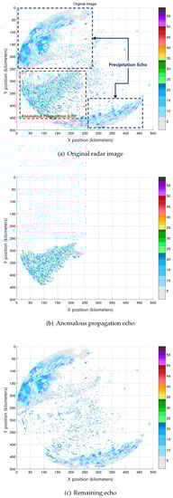
Figure 8.
Experimental results: Case 3.
5. Conclusions
In this paper, we proposed an ensemble classification method for distinguishing anomalous propagation echoes in radar observation data. Anomalous propagation echoes occur frequently and have characteristics fairly similar to precipitation. The echoes should be removed because they have a negative effect on quantitative precipitation estimation. Therefore, we implemented an ensemble classifier using actual appearance cases of anomalous propagation echoes as training and test data. The implemented ensemble classifier consisted of two major parts: the subset-selection method using the CRP and the base classifier using an artificial neural network. In the experiments, the suggested ensemble classifier showed 84.14% performance, which was about 2% higher than the k-means clustering-based ensemble classifier and about 4% higher than the standalone artificial neural network classifier.
In future work, we will continue to find ways to improve classification performance. First of all, we will examine influences of the class imbalance problem. Because it is an essential consideration to deal with real-world applications, we believe that it is possible to obtain better classification performance if we can solve the class imbalance problem: the imbalance ratio (IR) of the learning dataset for anomalous propagation echo is 2.41, which indicates that the dataset is imbalanced. We also think that selecting other kinds of base classifiers, such as support vector machine or decision trees, is another way to make the proposed method better. Moreover, considering that the final goal of the research is to identify all kinds of non-precipitation echoes using the proposed classifier, we will apply the suggested classifier to other representative non-precipitation echoes: spurious, interference patterns, biological, or other kinds of echoes. In addition, there are more ways to utilize radar data as classification inputs: obtain available data such as a correlation coefficient in dual polarization radar, use processed data such as an absolute radial velocity to consider a near-zero Doppler velocity property of the anomalous propagation echo, and so forth. We expect that these solutions mentioned above have positive effects on enhancing the performance of the proposed classifier.
Acknowledgments
This research was supported by the Basic Science Research Program through the National Research Foundation of Korea (NRF) funded by the Ministry of Education (NRF-2014R1A1A2056958).
Author Contributions
The work presented here was carried out in collaboration with all authors. Hansoo Lee designed, performed the experiments and wrote the manuscript; and Sungshin Kim contributed to the reviewing and revising of the manuscript.
Conflicts of Interest
The authors declare no conflict of interest.
References
- Merrill, I.S. Introduction to Radar Systems; Mc Graw-Hill: New York, NY, USA, 2001. [Google Scholar]
- Lakshmanan, V.; Fritz, A.; Smith, T.; Hondl, K.; Stumpf, G. An automated technique to quality control radar reflectivity data. J. Appl. Meteorol. Climatol. 2007, 46, 288–305. [Google Scholar] [CrossRef]
- Steiner, M.; Smith, J.A. Use of three-dimensional reflectivity structure for automated detection and removal of nonprecipitating echoes in radar data. J. Atmos. Ocean. Technol. 2002, 19, 673–686. [Google Scholar] [CrossRef]
- Pamment, J.; Conway, B. Objective identification of echoes due to anomalous propagation in weather radar data. J. Atmos. Ocean. Technol. 1998, 15, 98–113. [Google Scholar] [CrossRef]
- Berenguer, M.; Sempere-Torres, D.; Corral, C.; Sánchez-Diezma, R. A fuzzy logic technique for identifying nonprecipitating echoes in radar scans. J. Atmos. Ocean. Technol. 2006, 23, 1157–1180. [Google Scholar] [CrossRef]
- Cho, Y.H.; Lee, G.W.; Kim, K.E.; Zawadzki, I. Identification and removal of ground echoes and anomalous propagation using the characteristics of radar echoes. J. Atmos. Ocean. Technol. 2006, 23, 1206–1222. [Google Scholar] [CrossRef]
- Rico-Ramirez, M.A.; Cluckie, I.D. Classification of ground clutter and anomalous propagation using dual-polarization weather radar. IEEE Trans. Geosci. Remote Sens. 2008, 46, 1892–1904. [Google Scholar] [CrossRef]
- Da Silveira, R.B.; Holt, A.R. An automatic identification of clutter and anomalous propagation in polarization-diversity weather radar data using neural networks. IEEE Trans. Geosci. Remote Sens. 2001, 39, 1777–1788. [Google Scholar] [CrossRef]
- Grecu, M.; Krajewski, W.F. An efficient methodology for detection of anomalous propagation echoes in radar reflectivity data using neural networks. J. Atmos. Ocean. Technol. 2000, 17, 121–129. [Google Scholar] [CrossRef]
- Grecu, M.; Krajewski, W.F. Detection of anomalous propagation echoes in weather radar data using neural networks. IEEE Trans. Geosci. Remote Sens. 1999, 37, 287–296. [Google Scholar] [CrossRef]
- Peter, J.R.; Seed, A.; Steinle, P.J. Application of a Bayesian classifier of anomalous propagation to single-polarization radar reflectivity data. J. Atmos. Ocean. Technol. 2013, 30, 1985–2005. [Google Scholar] [CrossRef]
- Krajewski, W.F.; Vignal, B. Evaluation of anomalous propagation echo detection in WSR-88D data: A large sample case study. J. Atmos. Ocean. Technol. 2001, 18, 807–814. [Google Scholar] [CrossRef]
- Moszkowicz, S.; Ciach, G.J.; Krajewski, W.F. Statistical detection of anomalous propagation in radar reflectivity patterns. J. Atmos. Ocean. Technol. 1994, 11, 1026–1034. [Google Scholar] [CrossRef]
- Rahman, A.; Verma, B. Cluster-based ensemble of classifiers. Expert Syst. 2013, 30, 270–282. [Google Scholar] [CrossRef]
- Bishop, C.M. Neural Networks for Pattern Recognition; Oxford University Press: Oxford, UK, 1995. [Google Scholar]
- Pitman, J. Combinatorial Stochastic Processes; Springer: Berlin, Germany, 2002. [Google Scholar]
- Fabry, F.; Frush, C.; Zawadzki, I.; Kilambi, A. Extraction of near-surface index of refraction using radar phase measurements from ground targets. In Proceedings of the IEEE Antennas and Propagation Society International Symposium 1997: Digest, Montreal, QC, Canada, 13–18 July 1997; Volume 4, pp. 2625–2628.
- Lopez, P. A 5-yr 40-km-resolution global climatology of superrefraction for ground-based weather radars. J. Appl. Meteorol. Climatol. 2009, 48, 89–110. [Google Scholar] [CrossRef]
- Doviak, R.J.; Zrnic, D.S. Doppler Radar & Weather Observations; Academic Press: Cambridge, MA, USA, 2014. [Google Scholar]
- NASA Tropical Rainfall Measuring Mission, Radar Software Library. 2015. Available online: http://trmm-fc.gsfc.nasa.gov/trmm_gv/index.html (accessed on 9 July 2015).
- Kim, Y.H.; Kim, S.; Han, H.Y.; Heo, B.H.; You, C.H. Real-time detection and filtering of chaff clutter from single-polarization doppler radar data. J. Atmos. Ocean. Technol. 2013, 30, 873–895. [Google Scholar] [CrossRef]
- Schaefer, J.T. The critical success index as an indicator of warning skill. Weather Forecast. 1990, 5, 570–575. [Google Scholar] [CrossRef]
- Hyvärinen, O. A probabilistic derivation of Heidke skill score. Weather Forecast. 2014, 29, 177–181. [Google Scholar] [CrossRef]
- Lakshmanan, V.; Karstens, C.; Krause, J.; Tang, L. Quality control of weather radar data using polarimetric variables. J. Atmos. Ocean. Technol. 2014, 31, 1234–1249. [Google Scholar] [CrossRef]
© 2017 by the authors; licensee MDPI, Basel, Switzerland. This article is an open access article distributed under the terms and conditions of the Creative Commons Attribution (CC-BY) license (http://creativecommons.org/licenses/by/4.0/).