Article

Effects of Strong East Asian Cold Surges on Improving the Air Quality over Mainland China

1
State Key Laboratory of Loess and Quaternary, Institute of Earth Environment, Chinese Academy of Sciences, Xi’an 710061, China
2
College of Earth Science, University of Chinese Academy of Sciences, Beijing 100049, China
3
Chinese Academy of Sciences Center for Excellence in Tibetan Plateau Earth Sciences, Beijing 100101, China
*
Authors to whom correspondence should be addressed.
Atmosphere 2016, 7(3), 38; https://doi.org/10.3390/atmos7030038
Submission received: 27 December 2015 / Revised: 19 February 2016 / Accepted: 2 March 2016 / Published: 10 March 2016

Abstract

:
A strong East Asian cold surge (SEACS) is one of the most distinct extreme weather events that can promote an improvement in local air quality. Combining East Asian atmospheric circulation with the air pollution index (API) datasets of 47 major cities throughout mainland China in 11 winter half-years (November–March) during 2001/2002–2011/2012, we investigated the influence of 39 SEACSs in conjunction with air pollution episodes on air quality over mainland China. The results showed that SEACS can cause considerable improvement in air quality and a remarkable decrease in the API over mainland China in up to 4 days after the SEACS outbreak day. The removal efficiency of air pollutants by SEACSs was greater than 30% in north central China, eastern southwest China, and southeast China. The occurrence date of the lowest value of the local API (indicating the best local air quality) can be observed as late day by day from northwest to southeast over mainland China after the SEACS outbreak, indicating a process of gradual improvement in Chinese air quality after the SEACS outbreak. When clean cold air originating from Siberia moves southward into coastal areas of southeastern China, the increase in sea level pressure, the drop in temperature and the enhancement in the northerly wind also tend to progress gradually from north to south over SEACS-affected East Asia. Thus, the “early in the north and late in the south” feature of air quality improvement by SEACSs over mainland China results from the southward movement of cold air masses from high to low latitudes after cold surge outbreaks.

Graphical Abstract

1. Introduction

Since the 1980s, increasing anthropogenic emissions associated with rapid industrialization and urbanization, which changes the atmospheric composition and increases atmospheric particle concentration, have seriously degraded air quality over China [1,2,3,4]. In recent years, severe winter air pollution episodes or resultant low visibility events frequently occur in mainland China and have brought about serious impacts on air and ground traffic, human health, and the economy over China. Air pollution problems are receiving unprecedented attention in China [5,6,7].
Many previous studies have shown that weather-climate factors can play a substantial role in determining a regional short-term air quality. Anticyclonic synoptic systems can often lead to a low-level subsidence inversion, inhibit the vertical dispersion of pollutants (i.e., NOx, SO2, CO, O3, PM10, PM2.5), and subsequently influence local or regional air quality [8,9]. A stable weather condition with a high relative humidity also easily causes an accumulation of the regional air pollutants [10]. However, strong winds or heavy precipitation can reduce the concentration of air pollutants by diffusion or wet removal [11,12,13,14].
Cold surges, as a kind of typical synoptic process over East Asia, significantly affect the atmospheric circulation, resulting in improving local air quality [15]. Cold air originating from high-latitude Siberia can move from north to south into the southeastern coastal areas of China or even the equatorial regions as a cold surge outbreak [16,17,18]. With the arrival of a cold surge, there is a series of abrupt changes in meteorological factors such as a decrease in surface air temperature, a rise in sea-level air pressure, and a strengthening of northerly winds in the areas where the cold surge passes [19]. Lin et al. [20] examined the effect of cold surges on air quality over Taiwan from 1993 to 2005 and found that such events led to a decrease in the PM10 concentration and accordingly improved the local air quality. During cold surge occurrences, the arrival of fresh cold air may dissipate and reduce the local air pollutants [20]. Cheng et al. [21] used the WRF-Chem model to simulate and evaluate effects of cold surges on local air quality and found that a strong cold front activity has a cyclical effect of accumulation-transfer-removal-accumulation on air pollution. Qu et al. [22] deduced that the continuous decrease in the winter visibility over East China in recent years may be a result of a weakening in the East Asian Monsoon and the subsequent reduction in cold surge frequency with global warming. Clearly, cold surges play an important role in modulating air quality.
The previous research is mostly limited to a typical case study or a local scale cold surge, and few studies have identified strong cold surge effects on spatiotemporal variations in air quality on a large scale. Hence, in this study, we further investigate weather features of strong East Asian cold surge (SEACS) influences on air pollution over mainland China by combining meteorological data with air pollution data observed from Chinese major cities. The aim of this study is to deepen our understanding of the large-scale atmospheric circulation effect on modulating the regional air quality.

2. Data and Methods

2.1. Data

To analyze the characteristics of the atmospheric circulation associated with SEACS, we applied the latest ERA-interim global atmospheric reanalysis datasets with a 6-hour temporal resolution and a spatial resolution of 0.5 degrees from the European Center for Medium-Range Weather Forecasts [23]. The reanalysis dataset is a continually updated globally gridded dataset that represents the state of the Earth's atmosphere, incorporating observations and numerical weather prediction model output. In this work, we extracted daily sea level pressure (SLP), surface air temperatures, temperatures and meridional wind speed at 925 hPa from the datasets from 2001 to 2012.
To capture changes in air quality over China after the SEACS outbreaks, this study employed the daily Air Pollution Index (API) of major cities from the Ministry of Environmental Protection of the People’s Republic of China [24] throughout China from 2001 to 2012. API is a quantitative measure describing air pollution levels in China, by which air pollution data from several types of pollutants (including PM10, SO2, CO, O3 and NO2) are converted into a single value ranging from 0 to 500 [25]. Currently, only three pollutants including SO2, NO2 and PM10 are cited to the notification of API in China [26]. API, commonly used to report levels of ambient air pollution, is a simpler and more generalized way to provide timely information on air quality to the public than air pollutant concentrations, and API can help the public understand how local air quality changes over time. Here we selected 47 major Chinese cities (see Figure 1a and Supplementary Materials for the locations of 47 cities and provincial boundaries of mainland China) with the most complete data during 2001–2012.
In addition, we also applied daily aerosol optical depth (AOD) data at 550 nm from the Monitoring Atmospheric Composition and Climate project [27] from 2003 to 2012 to simply validate the API results analyzed.
We completed all analyses using the statistical software package IDL (version 8.1, ITT Visual Information Solutions), Origin 8.1 and ESRI Arcgis desktop 10.1.

2.2. Statistical Analysis Methods

We used composite analysis, a method widely used in research of atmospheric sciences as an important method of data analysis, to determine day-to-day variations in API from 47 major cities and SLP over the East Asian region during several days before and after the SEACS occurrences. According to all SEACSs identified (see Section 2.3 for the definition of SEACSs), we collected statistics of APIs or SLPs on the corresponding day preceding or following the SEACS outbreak day.
Clustering is a data mining technique by which similar data are put into related or homogeneous groups without advanced knowledge of the definitions of such groups [28]. As a special type of clustering, time series clustering has been used in diverse scientific fields to determine patterns and extract valuable information from complex and large datasets [29,30]. We applied the method to analyze API datasets related to the number of days preceding or following cold surge occurrences in 47 major cities throughout China to determine the days with the lowest API values after cold surge occurrences for these different cities. Firstly, we combined every 11-day data of APIs from all SEACS events to from a long API time series for each city. Secondly, we used the time series clustering to detect these data. Thirdly, according to the results of clustering and their contribution, we identified the day with the lowest API for each city. We then employed the Kriging method to interpolate the station data into gridded data with a resolution of 0.5° × 0.5°, and four regions were divided from north to south (see Section 3.2.2) according to the occurrence time of the lowest API values.
To investigate the southward trajectory of cold air masses after cold surge occurrences in conjunction with air pollution episodes on radioactivity levels, we adopted forward trajectories, which is a useful tool to identity the pathway of air mass movement. We computed 72 h kinematic 3D daily forward trajectories from the Siberian High during the cold surge outbreaks using the hybrid single-particle Lagrangian integrated trajectory model (version 4.9) [31] with the global reanalysis database developed by the Air Resources Laboratory from the National Oceanic and Atmospheric Administration[32] (see Section 3.3.3 for results).

2.3. Definition of SEACS

An abrupt drop in surface air temperature and an abnormal expansion of the Siberian High are important features of SEACSs. To describe these features, previous studies have proposed various synoptic criteria in identifying cold surges [18,33]. In this study, dates of SEACS occurrences were defined based on the method used by Panagiotopoulos et al. [34], Park et al. [16], and Huang et al. [35].
The intensity of the Siberian High usually serves as an indicator factor of the SEACS occurrence. A day of SEACS can be determined when the following three criteria are met simultaneously: (1) the daily mean SLP averaged for the Siberian High area (40°N to 65°N and 80°E to 120°E) is greater than 1035 hPa; (2) the daily minimum temperatures averaged for the SEACS-affected area (10°N to 54°N and 73°E to 135°E) is lower than 15 °C; and (3) the daily mean surface air temperature decreases by at least 4 °C compared to the previous day at more than 100 half-degree grid boxes within the SEACS affected area. These conditions ensure that the drop in temperature results from a large-scale synoptic process rather than a local effect, which means that SEACS was defined according to its affected and covered the geographic extent. Meanwhile, the above-mentioned consecutive SEACS days are combined as a SEACS event considering continuity of the cold surge process. The first day of the SEACS event is then defined as the outbreak day of the SEACS. Based on the above criteria, a total of 295 SEACS days were identified, and 83 SEACSs were detected from 2001 to 2012, an average of 7.5 SEACSs per year and 26.8 SEACS days per year.
We further identified SEACS events in conjunction with air pollution episodes. Based on China’s national average level of API (see Section 3.1) and durations of SEACSs, 39 SEACS events associated with air pollution episodes (the national API averaged for 5 consecutive days before the SEACS outbreak exceeding 80) were identified throughout the 11 winter seasons from 2001/2002 to 2011/2012.

3. Results

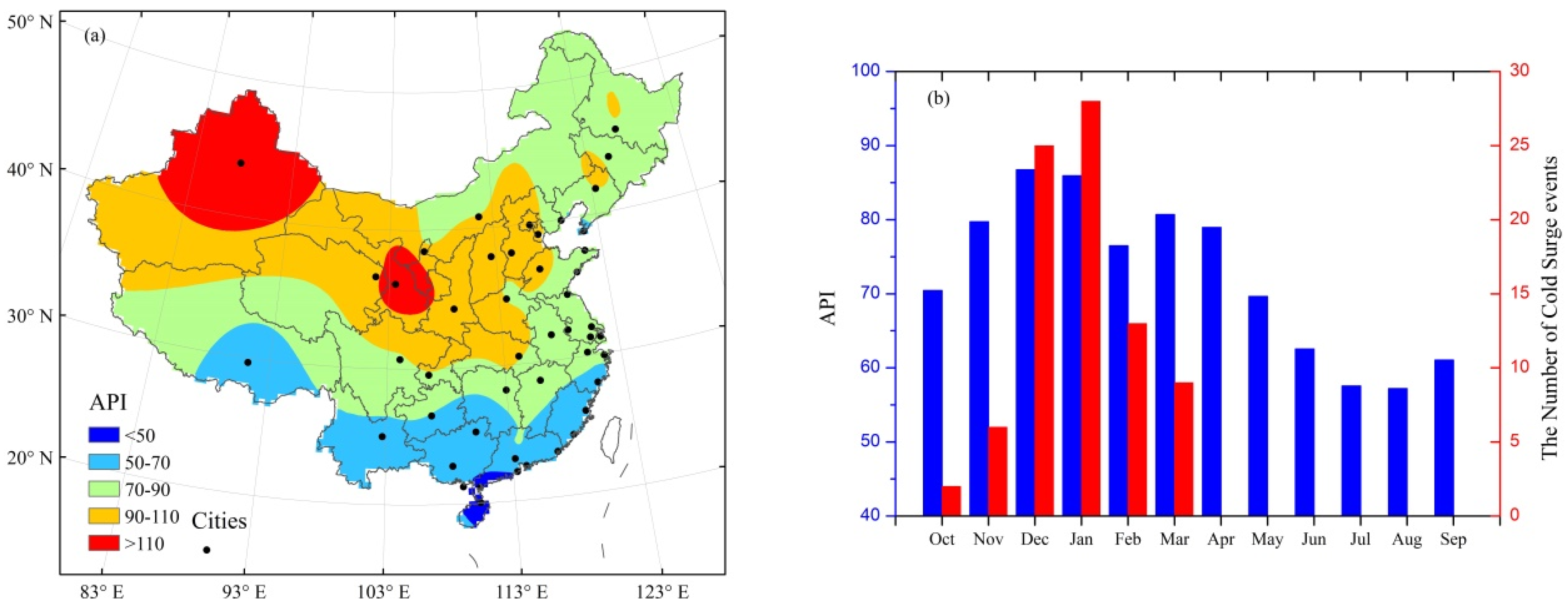
3.1. Activities SEACSs and Spatial Distribution of Air Quality over Mainland China

We conducted statistical analyses on the monthly cumulative frequency of SEACS occurrences and monthly API averaged for 47 major cities in China during 2001–2012. The results showed that SEACSs occurred mainly during wintertime from October to the following March. The 11-year cumulative frequency of SEACS events 25 times in December or January, an average of twice a month but only twice in October over a period of 11 years (Figure 1b). The best air quality detected occurred during the summer season. The air pollution in wintertime was serious in mainland China (Figure 1b), with a national average value of API higher than 80 in December or January. Due to the higher frequency of SEACSs (no SEACSs during the months of April to September) and poor air quality in wintertime, the winter half year (October–March) is the most suitable period to explore the effects of SEACSs on the regional air pollution in China. Hence, in this work, all the discussions, analyses, and data (including API and pollution) would be limited during the winter half year only. Additionally, as accidental extreme weather events for SEACSs, we focused on synoptic weather conditions associated with the impact of SEACSs on air quality over China.
Figure 1a shows the distribution of API averaged for 11 winters from 2001/2002 to 2011/2012 in China. There are higher API values in northern China north of ~30°N and lower API values in southern China, indicating worse air quality in the north than in the south. The regions with the worst air quality are concentrated mainly in northwest and north China, where the APIs are greater than 90, whereas the regions with the best air quality are located in the coast of southern China where the APIs range from 50 to 70. During wintertime, the high pollution in the northern areas is partly associated with coal-fired heating [36] as well as stable atmospheric stratification that inhibits the dispersion of air pollutants [10]. Additionally, the pollution in these areas also related to dust emission.
The wintertime geometric mean API of 47 cities is almost 80. The vast majority of cold surges usually pass though the Siberian area, leading the sea level pressure (SLP) rise. Based on the correlations of APIs in China with SLP in Siberia, we found that the correlations under the condition of poor air quality were higher, which showed that SEACSs had more significant impact on air quality. Hence, we focused on the impact of SEACSs (associated with poor air quality) on air quality. Hence, we took an average API greater than 80 as a criterion of the national air pollution episodes, and thus determined 39 SEACSs with air pollution during the 11 winter half-years. Table 1 lists the defining critical parameters of 39 SEACSs. Based on the persistent feature of the SEACS, the influential time of a typical SEACS is approximately 5 days [37]. As a result, we used the API values of 47 cities from day −5 (the 5th day before the SEACS outbreak day) to day 5 (the 5th day of the SEACS event including the outbreak day) to evaluate the effects of the SEACSs on air quality over China.

3.2. Air Quality Improvement by SEACSs

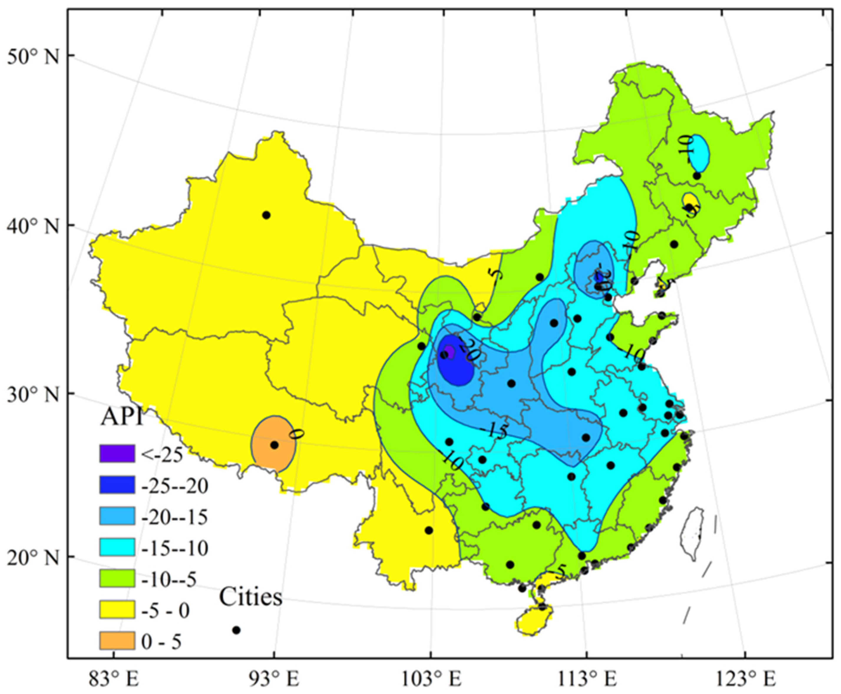
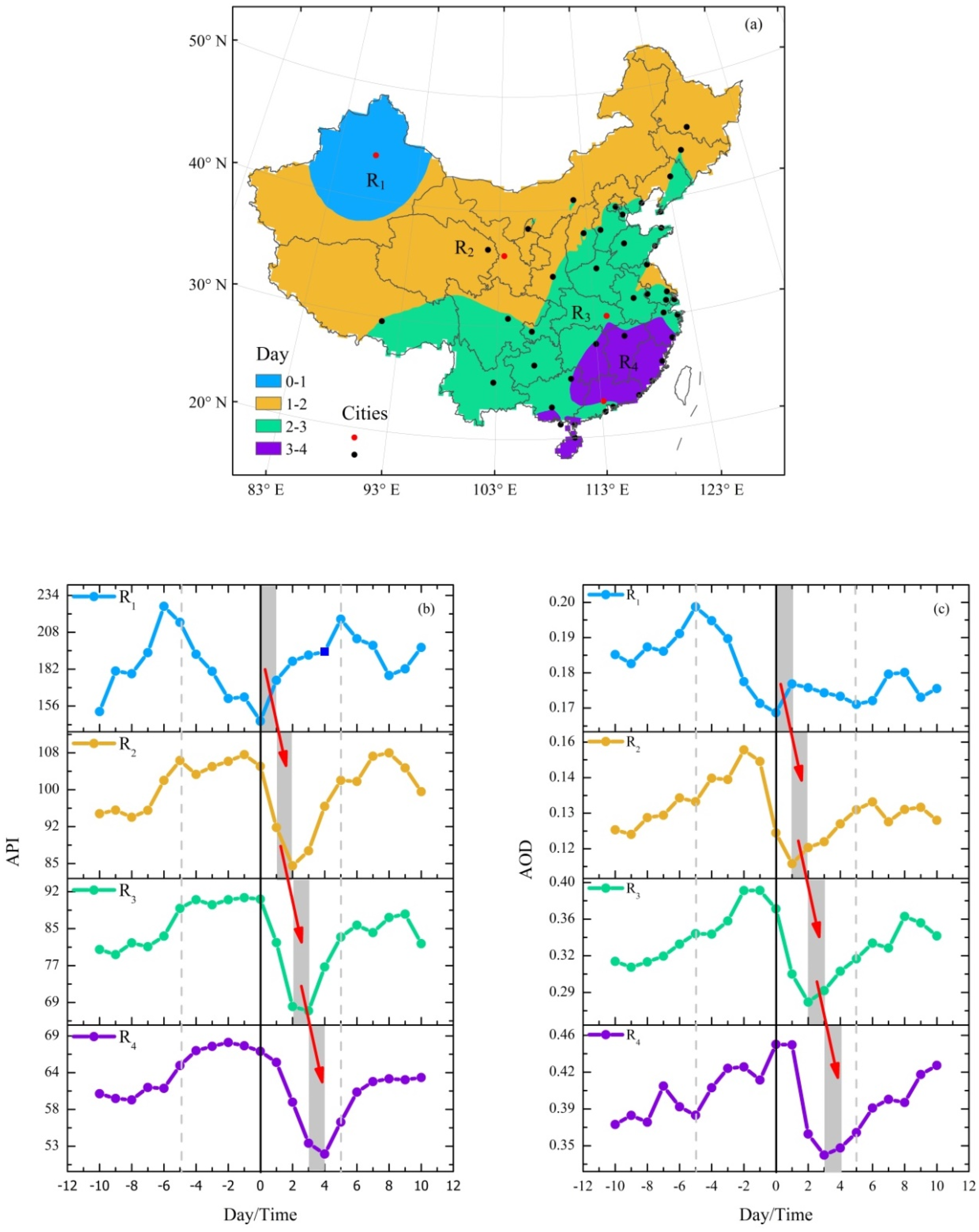
3.2.1. Spatial Features in Air Quality Improvement

We conducted a composite analysis of API relative to 39 SEACSs and investigated variation in API preceding and following SEACS occurrences to assess the improvement of air quality by SEACSs. The variation of 5-day averaged APIs after and before the SEACSs shows different degrees of decrease in API after SEACS occurrences in most parts of mainland China (Figure 2), which suggests that an improvement in air quality is induced by the SEACSs. Clean air brought by strong northwesterly winds with cold surges can remove the local air pollutants [15,20]. There is a relatively small decrease in API in western China west of 95°E, while considerable decreases in API are observed in mid-eastern China east of 95°E. A significant decline larger than 20 in API is concentrated mainly in the eastern Gansu Province, the mid-eastern region of Shaanxi Province, Hubei Province, northeastern Sichuan Province, the middle region of Shanxi Province, and the Jing-Jin-Ji region (see Figure S1 of Supplementary Materials). As seen, the air quality of eastern China is improved more than the air quality of western China, and the most improvement occurs in central China together with the arrivals of the SEACSs.
However, the above-mentioned API variation from the preceding 5-day average to the following 5-day average cannot reflect different temporal evolution patterns of air quality improvement in different regions of mainland China. Thus, we defined a removal efficiency index (hereinafter referred to as RE) by calculating a declining efficiency of API to better quantify air pollutant improvement under the influence of the SEACSs. When SEACS outbreak, the API is down and then up soon, especially in northwest China. We found that the 5-day mean conditions may underestimate the RE in northwest China, and not actually estimate the effect of SEACS on air quality. Indeed, the range of the maximum to the minimum value can more accurately and objectively estimate the RE in all cites. The RE is calculated by choosing the highest API and the lowest API as follows:
RE = ((APImax − APImin)/APImax)·100%
In Equation (1), APImax and APImin represent the highest API value in the preceding 5 days and the lowest API value in the following 5 days with respect to a cold surge outbreak. We calculated REs of 47 cities for 39 SEACSs in China and mapped the average RE distribution (Figure 3). REs of 20 cities are greater than 30%, and REs of 16 cities are between 20% and 30% in mainland China. RE exhibits an overall declining trend from north to south over mainland China. By conducting a comprehensive analysis of spatial distribution of the REs, higher REs (greater than 30%) were found in three regions, i.e., central north China (region A, including 5 observed cities), eastern southwest China (region B, including 5 observed cities), and southeastern China (region C, including 8 observed cities) (Figure 3). Table 2 further indicates API and RE variations in A, B, and C regions after and before SEACS occurrences. Before SEACS occurrences, the observed maximum API was 124 in region A, 91 in region B and 94 in region C. After SEACS outbreaks, the minimum APIs of 78, 59 and 65 occurred in regions A, B and C, respectively, showing dissimilar decreases, with the corresponding REs of 36.8%, 35.4% and 30.8%, respectively.

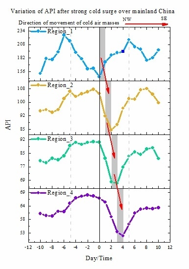
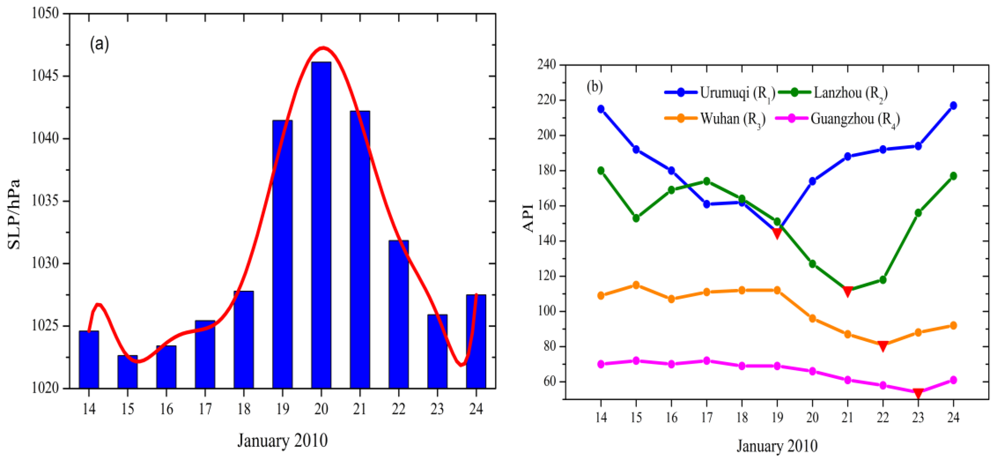
3.2.2. Temporal Evolution of Air Quality Improvement

To check the temporal evolution of air quality improvement by SEACSs over mainland China, we considered the occurrence of the lowest API (indicating the best air quality) after an SEACS outbreak as a significant signal of successful improvement in air quality. We combined every 11-day data of APIs from all SEACS events to from a long API time series for each city. Then time cluster analysis was used to identify and classify the dates with the lowest API from the API time series of 11 days centered on the SEACS outbreak days for the 47 cities. The results indicate that the occurrence date of minimum API values for different cities has a different lag time with respect to the SEACS outbreaks day. The dates with the lowest API were roughly divided into four time categories, corresponding to four regions (R1, R2, R3 and R4) in mainland China (Figure 4a). The occurrence date of the lowest API gradually becomes late day by day from northwest to southeast, indicating a process of gradual improvement in air quality after the SEACS outbreak. In R1 mostly concentrated within northern Xinjiang, the lowest API value occurred on the SEACS outbreak day (Day 0) to the first day after the SEACS outbreak (Day 1) (see Figure 4b). To depict the complete change process of API in detail in a longer time domain from 10 days before cold surge occurrence to 10 days after cold surge occurrence, we selected APIs value of 21day. In R2 mainly located in eastern Northwest China, northern North China and northeast China, the lowest API value occurred on Day 1 to Day 2 (the second day after the SEACS outbreak) (see Figure 4b). In R3 mainly located in southwest China, southern north China and the Yangtze River basin, the lowest API value occurred on Day 2 to the following day (Day 3). In R4 mostly concentrated in southeastern China south of the Yangtze River, the lowest API value was observed on Day 3 to the following day (Day 4) (see Figure 4b).
In addition, we analyzed the corresponding day-to-day variations of AOD for the four regions on the basis of data available throughout 2003–2011 and the associated 32 SEACS events. The lowest AOD also showed similar characteristics of spatiotemporal variation as API (see Figure 4c). The main reason for the time difference for air quality improvement is closely related to the southward movement of cold air masses from high latitudes after cold surge outbreaks, which is explained in detail in Section 3.3.
In the following, we took the SEACS that occurred on 19 January 2010, as a typical example case to concretely demonstrate the time difference of the air quality improvement induced by the SEACS in different regions. From day-to-day variations of SLP averaged for the Siberian High area (Figure 5a), the SLP was lower than 1030 hPa before 19 January 2010. On 19 January 2010, the SLP dramatically increased over 1040 hPa, reaching the corresponding criterion for the SEACS. The SLP remained at a high level for three days and then rapidly declined. From northwest to southeast, we chose Urumqi, Lanzhou, Wuhan, and Guangzhou, which belonged to R1, R2, R3, and R4, respectively, as representative cities of the four regions to observe their air quality variation. The lowest API value occurred on 19 January at Urumqi, on 21 January at Lanzhou, on 22 January at Wuhan and on 23 January at Guangzhou (Figure 5b). This case visually displayed the SEACS effect on improving air quality and up to 4 days of its stepwise time lag from the northwest to the southeast of China.
Actually, we also analyzed the interannual variations of frequency of cold surge and API during wintertime from 2001/2002 to 2011/2012, and found no clear relationship between them. Although there is a decline trend in API, no corresponding increase trend in the frequency of SEACSs is observed. This situation may mean that the long-term improvement of air quality have included the contribution of increasing air pollution control. Additionally, the year-to-year correlation between the frequency of cold surge and API is not signification (R = 0.034). A SEACS, as an occasional extreme weather event, has a short life cycle and effective time. Thus, activities of SEACSs hardly control seasonal-scale API variations. Based on the above, this study does not explicitly consider the impact of cold surge on air quality at inter-annual scale.

3.2.3. Removal Effect of SEACSs on Air Pollutants in Different Regions

To further detect the removal effect of SEACSs on air pollutants in different regions, we also analyzed API variations in R1, R2, R3, and R4 regions during five days preceding and following SEACS outbreaks based on composite analysis of 39 SEACS events. As indicated in Table 3, APIs were all reduced by SEACSs in the four different regions, and the corresponding REs showed a sequential arrangement, i.e., R1 > R2 > R3 > R4, with the highest RE value (35.8%) in R1 and the lowest (25.4%) in R4. The improvement effect of SEACSs on air quality gradually weakens from northwest to southeast because the intensity of the Siberian High continues to decay, and the cleanliness of the corresponding cold air continuously declines during the course of the NW-SE oriented movement of the Siberian High or cold air mass after the SEACS outbreaks.

3.3. Temporal Evolution of Weather Factors Associated with SEACSs

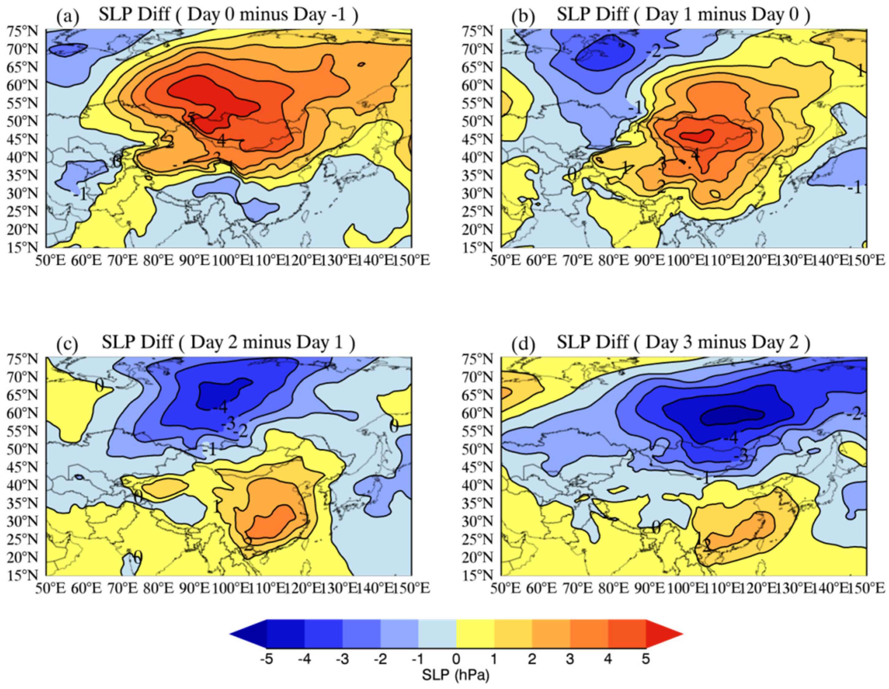
3.3.1. Dynamic Changes of SLP

As a result of SEACSs, API declined and air quality was improved in China. During the SEACS occurrences, spatiotemporal differences in removal effects of SEACSs on air pollutants over China were closely associated with the southeastward movement of the cold air mass under the guidance of the Siberian High [20]. To track the movement of the cold air mass, we examined SLP dynamic changes during SEACSs. Figure 6 illustrates 39 SEACS composite distributions of daily SLP on 4 consecutive days from the SEACS outbreak day. On Day 0 (the SEACS outbreak day), a strong and large Siberian High appeared in Eurasia. Junggar Basin, Xinjiang, Inner Mongolia, North China and Northeast China are basically controlled by high pressure, with the isobar of 1026 hPa extending southward into the Bohai Sea (Figure 6a). On Day 1 (the first day after the SEACS outbreak), the High was enhanced at the center and expanded outwards. The isobar of 1026 hPa shifted southward to the lower reaches of the Yangtze River (Figure 6b). One day later, the High continued to move southward. However, its intensity became weak and its extent began to shrink slightly (Figure 6c). On the following day, the intensity of the High decreased significantly, and the area with SLP higher than 1038 hPa shrank to western Mongolia, although the isobar of 1026 hPa shifted southward to South China (Figure 6d). On Day 4 (the fourth day after the SEACS outbreak, not shown), the southward movement continued but not strongly. In summary, with the southward movement of the Siberian High during SEACSs, clean air was advected in a stepwise manner to mainland China from northwest to southeast, leading the successive improvement of air quality in the R1, R2, R3 and R4 regions.
To further investigate the dynamic changes of SLP during SEACSs, we used the SLP difference (∆SLP) between a specific day and its previous day on the basis of composite analyses of 39 SEACSs to reflect the inter-day variation of the SLP. On the SEACS outbreak day (Figure 7a), the SLP significantly increased in Siberia compared with the preceding day, and ∆SLP exceeded 5 hPa in central Siberia. The isoline of zero was close to the Yangtze River, implying that areas south of the Yangtze River were unaffected by the SEACS on the same day. On Day 1 (Figure 7b), the isoline of zero occurred in the South China coast areas, and the whole of China was intruded by cold air. The central area of positive ΔSLP greater than 4 hPa moved into Mongolia though its extent narrowed. On Day 2 (Figure 7c), the center of the positive ∆SLP moved into the southern region of the Yangtze River. On Day 3 (Figure 7d), a positive ∆SLP center appeared in southern China, but its intensity was weakened while a negative ∆SLP center appeared in Siberia. From Day 0 to Day 3, the center of the positive ∆SLP moved significantly southwards from Siberia to southern China. On Day 4 (not shown), a smaller positive ∆SLP center still existed near the south China coastal areas. The results also show a day-by-day southward movement feature of the high-pressure system or cold air mass in pace with the SEACS outbreak and development, which eventually determines the spatiotemporal variations in the removal effects of SEACSs on air pollutants over mainland China.

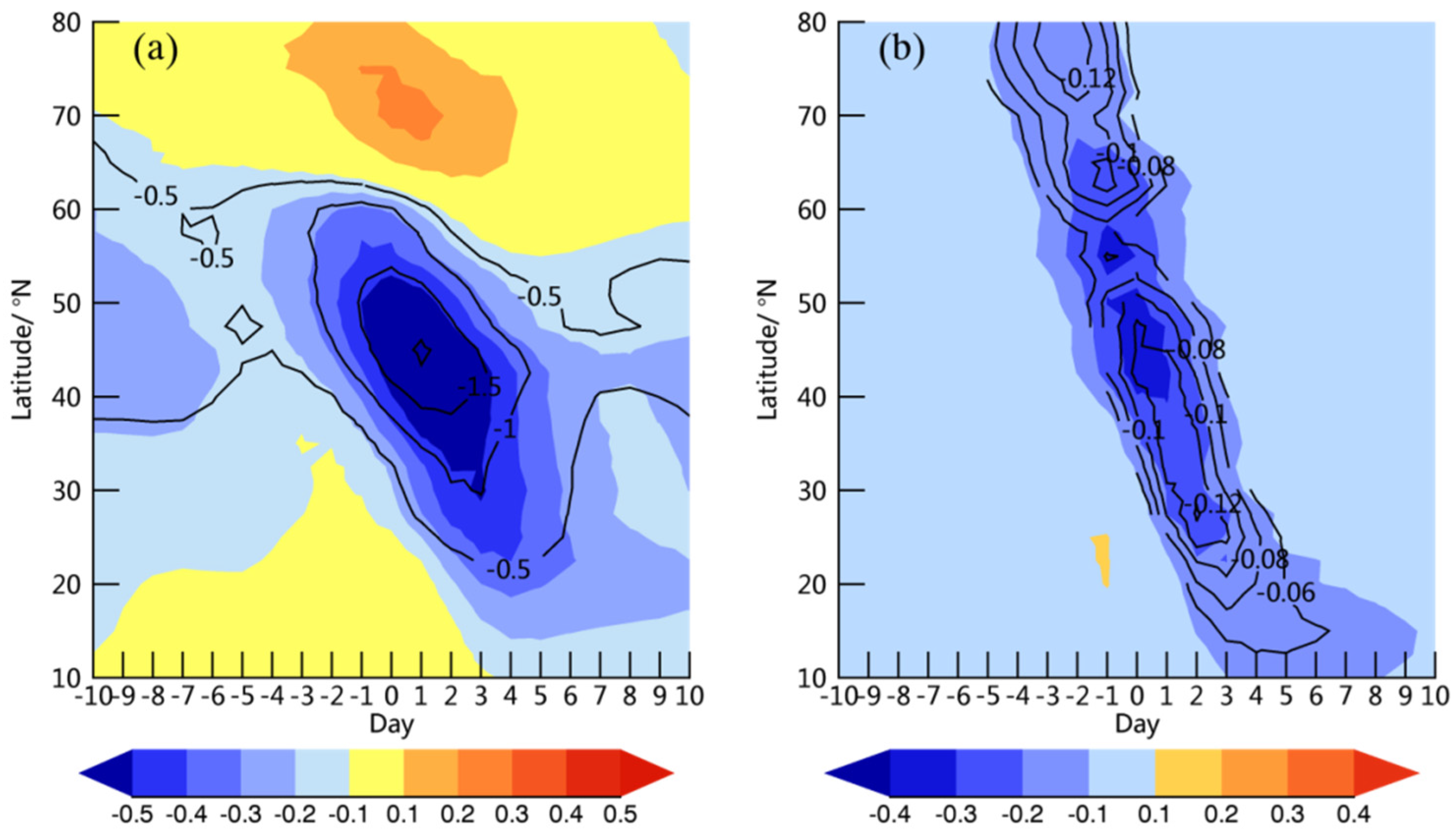
3.3.2. Temporal Evolution of Temperature and Meridional Wind at 925 hPa

To further understand the progress of improving air quality by SEACS day by day, we investigated temporal evolution features of temperature and meridional wind at 925 hPa during the SEACS occurrences. Southward-moving Siberian air masses related to SEACSs can not only induce the SLP variations but also cause significant changes in temperature and meridional wind in the regions affected by the SEACSs. Hence, applying the method of Shoji et al. [34], we checked the variations of correlations between the 925 hPa temperature zonally averaged for 90–135 °E and SLP averaged for the Siberian High area with latitude and time. Figure 8a illustrates that there was a significantly negative correlation between the SLP and the following lower-tropospheric temperature over East Asia, indicating the subsequent declines of the temperature from north to south over East Asia with the development of the Siberian High and the southward movement of cold air masses during the SEACSs, especially over the period of Day −1 to Day 4. The temperature change rate (slope for regression) also showed corresponding spatiotemporal characteristics.
At the same time, Figure 8b demonstrates a significant negative correlation between the SLP and lower-tropospheric meridional wind over East Asia, which indicated a process of the subsequent strengthening in northerly wind speed from north to south over East Asia, from the preceding days to the following days of SEACS outbreaks. According to a study by Lin et al. [16], an increase in the northerly wind speed can promote the diffusion of local air pollutants and improve local air quality during the SEACS occurrences [16]. Thus, strong winds are favorable for removal of air pollutants during SEACSs [38]. Moreover, the subsequent strengthening in the northerly wind speed from north to south is a direct reason for spatiotemporal differences in air quality improvement by SEACSs over mainland China.

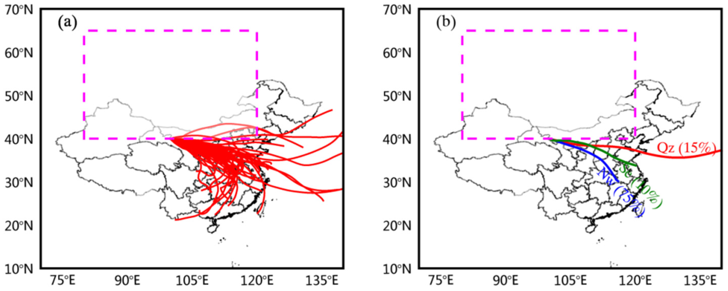
3.3.3. Trajectory of SEACSs

We further analyzed the moving paths of cold air originating from the Siberian region after SEACS occurrences by using forward trajectory analysis. From a central point (100°E, 40°E) on the southern boundary of the Siberian region at an altitude of 2500 m, 72-h forward trajectories of air particles were tracked after the 39 SEACS outbreaks (Figure 9a).
We further used cluster analysis to classify the forward trajectories of 39 SEACSs and obtained three main paths (Figure 9b). The quasi-zonal path accounted for 15% while the other two paths took the northwest-southeast orientation and arrived to the lower reaches of the Yangtze River or South China, accounting for 10% and 75%, respectively. Thus, most SEACSs move from northwest to southeast and consequently improve air quality over mainland China.
The trajectory map of cold air masses in the original manuscript was only used to depict the movement of cold air masses originating from Serbian area to southern East Asia, which does not demonstrate the cold surge tracks to R1 and R2. However, the map is only a schematic diagram of the movement of cold air masses. In fact, the trajectories are related to the locations of the tracer starting points. For example, if we select other locations as tracer starting points, the tracks of cold air masses can reach Northwest China and influence air quality there.

4. Discussion

Although previous researches [15,20,21] based on case studies have noticed the relationship of cold surges with East Asian air quality, this study further investigates the important controlling effect of East Asian cold surge on improving winter air quality in mainland China through comprehensive integration of 39 SEACS events. The composite analyses of SLP, lower-tropospheric temperature and meridional wind show that the development of SEACSs after the outbreak is a gradual movement process of high-latitude cold air masses from north to south, which leads to transport and dispersion of air pollutants, and eventually improvement air quality over East Asia. It is the movement of cold air masses that causes the spatiotemporal difference of air quality improvement with the feature of “early in the north and late in the south”. These results will help to further recognize the change of East Asian atmospheric environment and promote the short-term forecast level of air pollution in China.
Due to the limitation of the API data length, the interannual or decadal change of SEACS influence on air quality has not been discussed in this paper. In fact, SEACSs have obvious interannual and interdecadal variation characteristics [16,22,39,40]. For example, a weakening of the East Asian winter monsoon related to the global warming may have reduced the intensity and frequency of cold waves over East Asia in recent years [41,42]. Meanwhile, the situation of air pollution is recently becoming more and more serious in some places of China [10,43]. Although increasingly frequent air pollution events may be associated with raising emissions of pollutants caused by the economy development and human activities, it is not clear whether the recent deterioration in winter air quality over mainland China is related to the reduction of SEACSs. Furthermore, the weakening of East Asian winter monsoon or cold surge processes is likely to continue in the future with global warming [16,44]. The significant change in meteorological factors associated with local air quality at various time scales and its implications on the regional climate change are worthy of further study.
Given that strong cold surges have a larger impact on air quality in broad geographical areas, normal cold surges (weak cold surges) has not been discussed in this paper. Recently, there were frequent incidents of large-area haze weather during wintertime over China. Although a cold surge can improve air quality no matter how strong or weak it is, as a large-area air pollution episode, a strong cold surge can improve air quality in larger area, while a normal cold surge can only improve local air quality.
The study results in this paper provide a preliminary climatological-statistical analysis of SEACSs on improving Chinese air quality. These results need be further verified with the relevant numerical simulation experiments to deeply understand their causal relationships and underlying mechanisms. In consideration of the time-lag correlation between SLP in Siberian High area and API in the downstream regions including China, it is of practical significance to develop a statistical or dynamic-statistic short-term forecast model of air pollution for some specific regions of China in the future.

5. Conclusions

By combining ERA-Interim atmospheric reanalysis with Chinese API datasets, we investigated the effects of the SEACS on improving the air quality over mainland China based on 39 SEACS events in conjunction with air pollution episodes during 11 winter half-years (October–March) from 2001/2002 to 2011/2012. We have demonstrated that SEACSs can significantly improve the air quality over China for up to 4 days after the SEACS outbreak day. The removal efficiency for air pollutants by SEACSs is greater than 30% in three regions, i.e., central North China, eastern Southwest China and southeastern China. The occurrence date of the lowest value of the local API (indicating the best local air quality) can be observed to become later day by day from the northwest to the southeast over mainland China after an SEACS outbreak, indicating a process of gradual improvement in Chinese air quality after the SEACS outbreak. For example, there is a minimum API in northern Xinjiang on the SEACS outbreak day while a minimum API occurs in southeastern China south of the Yangtze River on the third day to fourth day after the SEACS outbreak. Meanwhile, the SEACS-induced increase in SLP, the drop in temperature and the enhancement in northerly wind also tend to be postponed gradually from north to south over the SEACS-affected East Asia after SEACS outbreaks. Thus, the “early in the north and late in the south” feature of air quality improvement by SEACS over mainland China results from the southward movement of cold air masses from high to low latitudes after cold surge outbreaks.

Supplementary Materials

The following are available online at www.mdpi.com/2073-4433/7/3/38/s1, Figure S1: Map of provincial boundaries of mainland China; Table S1: Locations of 47 cities in mainland China.

Acknowledgments

This work was supported by the Strategic Priority Research Program of the Chinese Academy of Sciences (XDA05110101) and the National Science Foundation of China (41572150, 41290255). The authors are grateful to the Ministry of Environmental Protection of China for the air quality data (http://datacenter.mep.gov.cn) and to the European Center for Medium-Range Weather Forecasts for the ERA-Interim reanalysis data (http://apps.ecmwf.int/datasets/).

Author Contributions

Zhaosheng Wang and Xiaodong Liu conceived this study; Zhaosheng Wang collected the data, generated the figures, analyzed the results and drafted the paper; Xiaodong Liu and Xiaoning Xie also contributed to analyzing the results and improving the manuscript.

Conflicts of Interest

The authors declare no conflict of interest.

Abbreviations

The following abbreviations are used in this manuscript:
SEACSStrong East Asian Cold Surge
APIAir Pollution Index
RERemoval Efficiency
SLPSea Level Pressure
AODAerosol Optical Depth

References

  1. Qian, Y.; Gong, D.; Fan, J.; Leung, L.R.; Bennartz, R.; Chen, D.; Wang, W. Heavy pollution suppresses light rain inChina: Observations and modeling. J. Geophys. Res. 2009, 114. [Google Scholar] [CrossRef]
  2. Wang, K.C.; Dickinson, R.E.; Liang, S.L. Clear sky visibility has decreased over land globally from 1973 to 2007. Science 2009, 323, 1468–1470. [Google Scholar] [CrossRef] [PubMed]
  3. Monks, P.; Granier, C.; Fuzzi, S.; Stohl, A.; Williams, M.; Akimoto, H.; Amann, M.; Baklanov, A.; Baltensperger, U.; Bey, I. Atmospheric composition change–Global and regional air quality. Atmos. Environ. 2009, 43, 5268–5350. [Google Scholar] [CrossRef]
  4. Seinfeld, J.H.; Pandis, S.N. Atmospheric Chemistry and Physics: From Air Pollution to Climate Change; John Wiley & Sons: Hoboken, NJ, USA, 2012. [Google Scholar]
  5. Tao, M.; Chen, L.; Xiong, X.; Zhang, M.; Ma, P.; Tao, J.; Wang, Z. Formation process of the widespread extreme haze pollution over northern Chinain January 2013: Implications for regional air quality and climate. Atmos. Environ. 2014, 98, 417–425. [Google Scholar] [CrossRef]
  6. Boynard, A.; Clerbaux, C.; Clarisse, L.; Safieddine, S.; Pommier, M.; Van Damme, M.; Bauduin, S.; Oudot, C.; Hadji-Lazaro, J.; Hurtmans, D.; et al. First simultaneous space measurements of atmospheric pollutants in the boundary layer from iasi: A case study in the north China plain. Geophys. Res. Lett. 2014, 41, 645–651. [Google Scholar] [CrossRef]
  7. Chen, W.; Yan, L.; Zhao, H. Seasonal variations of atmospheric pollution and air quality in Beijing. Atmosphere 2015, 6, 1753–1770. [Google Scholar] [CrossRef]
  8. Xu, J.; Yan, F.; Xie, Y.; Wang, F.; Wu, J.; Fu, Q. Impact of meteorological conditions on a nine-day particulate matter pollution event observed in December 2013, Shanghai, China. Particuology 2015, 20, 69–79. [Google Scholar] [CrossRef]
  9. Wu, M.; Wu, D.; Fan, Q.; Wang, B.M.; Li, H.W.; Fan, S.J. Observational studies of the meteorological characteristics associated with poor air quality over the Pearl River Deltain China. Atmos. Chem. Phys. 2013, 13, 10755–10766. [Google Scholar] [CrossRef]
  10. Liu, X.; Hui, Y.; Yin, Z.-Y.; Wang, Z.; Xie, X.; Fang, J. Deteriorating haze situation and the severe haze episode during December 18–25 of 2013 in Xi’an China, the worst event on record. Theor. Appl. Climatol. 2015. [Google Scholar] [CrossRef]
  11. Jones, A.M.; Harrison, R.M.; Baker, J. The wind speed dependence of the concentrations of airborne particulate matter and Nox. Atmos. Environ. 2010, 44, 1682–1690. [Google Scholar] [CrossRef]
  12. Wang, Z.B.; Hu, M.; Wu, Z.J.; Yue, D.L.; He, L.Y.; Huang, X.F.; Liu, X.G.; Wiedensohler, A. Long-term measurements of particle number size distributions and the relationships with air mass history and source apportionment in the summer of Beijing. Atmos. Chem. Phys. 2013, 13, 10159–10170. [Google Scholar] [CrossRef]
  13. Malek, E.; Davis, T.; Martin, R.S.; Silva, P.J. Meteorological and environmental aspects of one of the worst national air pollution episodes (January 2004) in Logan, Cache Valley, Utah, USA. Atmos. Res. 2006, 79, 108–122. [Google Scholar] [CrossRef]
  14. Chaloulakou, A.; Kassomenos, P.; Spyrellis, N.; Demokritou, P.; Koutrakis, P. Measurements of PM10 and PM2.5 particle concentrations in Athens, Greece. Atmos. Environ. 2003, 37, 649–660. [Google Scholar] [CrossRef]
  15. Hien, P.D.; Loc, P.D.; Dao, N.V. Air pollution episodes associated with East Asian winter monsoons. Sci. Total. Environ. 2011, 409, 5063–5068. [Google Scholar] [CrossRef] [PubMed]
  16. Park, T.W.; Ho, C.H.; Jeong, S.J.; Choi, Y.S.; Park, S.K.; Song, C.K. Different characteristics of cold day and cold surge frequency over East Asianin a global warming situation. J. Geophys. Res. 2011, 116. [Google Scholar] [CrossRef]
  17. Zhang, Y.; Sperber, K.R.; Boyle, J.S. Climatology and interannual variation of the East Asian winter monsoon: Results from the 1979–95 NCEP/NCAR reanalysis. Mon. Weather Rev. 1997, 125, 2605–2619. [Google Scholar] [CrossRef]
  18. Jeong, J.H.; Ho, C.H. Changes in occurrence of cold surges over East Asia in association with arctic oscillation. Geophys. Res. Lett. 2005, 32. [Google Scholar] [CrossRef]
  19. CCiM, G.R. The horizontal and vertical structure of East Asia winter monsoon pressure surges. QJR Meteorol. Soc. 1999, 125, 29–54. [Google Scholar]
  20. Lin, C.-Y.; Lung, S.-C.C.; Guo, H.-R.; Wu, P.-C.; Su, H.-J. Climate variability of cold surge and its impact on the air quality of Taiwan. Clim. Chang. 2008, 94, 457–471. [Google Scholar] [CrossRef]
  21. Cheng, N.L.; Meng, F.; Xu, J.; He, Y.J. Process analysis about the impact of a strong cold front on air pollution transportation in eastern China in spring. Res. Environ. Sci. 2013, 26, 34–42. (In Chinese) [Google Scholar]
  22. Qu, W.; Wang, J.; Zhang, X.; Yang, Z.; Gao, S. Effect of cold wave on winter visibility over eastern China. J. Geophys. Res. 2015, 120, 2394–2406. [Google Scholar] [CrossRef]
  23. Dee, D.P.; Uppala, S.M.; Simmons, A.J.; Berrisford, P.; Poli, P.; Kobayashi, S.; Andrae, U.; Balmaseda, M.A.; Balsamo, G.; Bauer, P.; et al. The era-interim reanalysis: Configuration and performance of the data assimilation system. QJR Meteorol. Soc. 2011, 137, 553–597. [Google Scholar] [CrossRef]
  24. Chinese Minstry of Environmental Protection (MEP). Available online: http://datacenter.mep.gov.cn (accessed on 5 August 2015).
  25. Li, L.; Qian, J.; Ou, C.Q.; Zhou, Y.X.; Guo, C.; Guo, Y. Spatial and temporal analysis of air pollution index and its timescale-dependent relationship with meteorological factors in Guangzhou, China, 2001–2011. Environ. Pollut. 2014, 190, 75–81. [Google Scholar] [CrossRef] [PubMed]
  26. Deng, J.; Wang, T.; Jiang, Z.; Xie, M.; Zhang, R.; Huang, X.; Zhu, J. Characterization of visibility and its affecting factors over Nanjing, China. Atmos. Res. 2011, 101, 681–691. [Google Scholar] [CrossRef]
  27. Inness, A.; Baier, F.; Benedetti, A.; Bouarar, I.; Chabrillat, S.; Clark, H.; Clerbaux, C.; Coheur, P.; Engelen, R.J.; Errera, Q.; et al. The MACC reanalysis: An 8 year data set of atmospheric composition. Atmos. Chem. Phys. 2013, 13, 4073–4109. [Google Scholar] [CrossRef] [Green Version]
  28. Rai, R.S. A survey of clustering techniques. Int. J. Comput. Appl. 2010, 7, 5. [Google Scholar] [CrossRef]
  29. Pereira, M.G.; Caramelo, L.; Orozco, C.V.; Costa, R.; Tonini, M. Space-time clustering analysis performance of an aggregated dataset: The case of wildfires in Portugal. Environ. Modell. Softw. 2015, 72, 239–249. [Google Scholar] [CrossRef]
  30. Gómez-Losada, Á.; Pires, J.C.M.; Pino-Mejías, R. Time series clustering for estimating particulate matter contributions and its use in quantifying impacts from deserts. Atmos. Environ. 2015, 117, 271–281. [Google Scholar] [CrossRef]
  31. Draxler, R.; Rolph, G. Cited 2003: HYSPLIT (Hybrid Single-Particle Lagrangian Integrated Trajectory) Model; NOAA/Air Resources Laboratory, Silver Spring: College Park, MD, USA, 2003.
  32. Stein, A.; Draxler, R.; Rolph, G.; Stunder, B.; Cohen, M.; Ngan, F. Noaa’s hysplit atmospheric transport and dispersion modeling system. Bull. Am. Meteorol. Soc. 2015, 96, 2059–2077. [Google Scholar] [CrossRef]
  33. Chen, T.C.; Yen, M.C.; Huang, W.R.; Gallus, W.A. An East Asian cold surge: Case study. Mon. Weather Rev. 2002, 130, 2271–2290. [Google Scholar] [CrossRef]
  34. Panagiotopoulos, F.; Shahgedanova, M.; Hannachi, A.; Stephenson, D.B. Observed trends and teleconnections of the Siberian high: A recently declining center of action. J. Clim. 2005, 18, 1411–1422. [Google Scholar] [CrossRef]
  35. Huang, W.-R.; Wang, S.-Y.; Chan, J.C.L. Discrepancies between global reanalyses and observations in the interdecadal variations of southeast Asian cold surge. Int. J. Climatol. 2011, 31, 2272–2280. [Google Scholar] [CrossRef]
  36. Chan, C.K.; Yao, X. Air pollution in mega cities in China. Atmos. Environ. 2008, 42, 1–42. [Google Scholar] [CrossRef]
  37. Shoji, T.; Kanno, Y.; Iwasaki, T.; Takaya, K. An isentropic analysis of the temporal evolution of East Asian cold air outbreaks. J. Clim. 2014, 27, 9337–9348. [Google Scholar] [CrossRef]
  38. Ashfold, M.J.; Pyle, J.A.; Robinson, A.D.; Meneguz, E.; Nadzir, M.S.M.; Phang, S.M.; Samah, A.A.; Ong, S.; Ung, H.E.; Peng, L.K.; et al. Rapid transport of East Asia pollution to the deep tropics. Atmos. Chem. Phys. 2015, 15, 3565–3573. [Google Scholar] [CrossRef]
  39. Chen, T.-C.; Huang, W.-R.; Yoon, J.-H. Interannual variation of the East Asia cold surge activity. J. Clim. 2004, 17, 401–413. [Google Scholar] [CrossRef]
  40. Woo, S.H.; Kim, B.M.; Jeong, J.H.; Kim, S.J.; Lim, G.H. Decadal changes in surface air temperature variability and cold surge characteristics over northeast Asia and their relation with the arctic oscillation for the past three decades (1979–2011). J. Geophys. Res. 2012, 117. [Google Scholar] [CrossRef]
  41. Hu, Z.Z.; Bengtsson, L.; Arpe, K. Impact of global warming on the Asian winter monsoon in a coupled GCM. J. Geophys. Res. 2000, 105, 4607–4624. [Google Scholar] [CrossRef]
  42. Ding, Y.; Liu, Y.; Liang, S.; Ma, X.; Zhang, Y.; Si, D.; Liang, P.; Song, Y.; Zhang, J. Interdecadal variability of the East Asian winter monsoon and its possible links to global climate change. J. Meteor. Res. 2014, 28, 693–713. [Google Scholar] [CrossRef]
  43. Zhang, X.; Wang, Y.; Niu, T.; Zhang, X.; Gong, S.; Zhang, Y.; Sun, J. Atmospheric aerosol compositions in China: Spatial/temporal variability, chemical signature, regional haze distribution and comparisons with global aerosols. Atmos. Chem. Phys. 2012, 12, 779–799. [Google Scholar] [CrossRef]
  44. Hori, M.E.; Ueda, H. Impact of global warming on the east asian winter monsoon as revealed by nine coupled atmosphere-ocean GCMs. Geophys. Res. Lett. 2006, 33. [Google Scholar] [CrossRef]
Figure 1. (a) Spatial distribution of API averaged for 11 winter half-years (October-March) throughout 2001/2002–2011/2012 in China, black dots indicate 47 cities (see Table S1); (b) Annual cycles of monthly cumulative frequency of SEACS occurrences and monthly API geometrically averaged for 47 major cities in China during 2001–2012.
Atmosphere 07 00038 g001
Figure 2. The 39 SEACS composited distributions of the difference between API averaged for 5 consecutive days from the SEACS outbreak day and API averaged for the 5th–1st days before the SEACS outbreak.
Atmosphere 07 00038 g002
Figure 3. Distribution of the 39-case averaged removal efficiency (RE) of SEACSs on air pollutants over mainland China. The A, B, and C with the higher removal efficiency indicate central north China, eastern southwest China, and southeastern China, respectively.
Atmosphere 07 00038 g003
Figure 4. (a) Clustering analysis obtained distribution map of the occurrence time of the lowest API with respect to the SEACS outbreak. Day 0 indicates the SEACS outbreak day. Day 1, 2, 3 and 4 indicate the 1st, 2nd, 3rd and 4th day after the SEACS outbreak day, respectively; red dots indicate 4 representative cities (Urumqi, Lanzhou, Wuhan and Guangzhou) from different regions); black dots indicate 47 cities; (b) 39 SEACS composited day-to-day variations of geometric mean API in different regions (R1, R2, R3 and R4) during 21 days before and after the SEACS outbreak. The negative (positive) value in x-axis indicates the time leading (lagging) the SEACS outbreak day; and (c) same as (b) but for 32 SEACS composited day-to-day variations of geometric mean AOD.
Atmosphere 07 00038 g004
Figure 5. Day-to-day variations of daily SLP averaged for the Siberian High area (a); and API at four representative cities (Urumqi, Lanzhou, Wuhan and Guangzhou) from different regions (b) in a typical example case of SEACS with air pollution. The date of the SEACS outbreak was January 19, 2010. The locations of the four cities are shown in Figure 4a. The red inverted triangles indicate the dates with the lowest API in (b).
Atmosphere 07 00038 g005
Figure 6. The 39 SEACS composited distributions of daily mean sea level pressure (SLP, unit: hPa) in 4 consecutive days from the SEACS outbreak day. (a) Day 0; (b) Day 1; (c) Day 2; and (d) Day 3. The meaning of Day 0–Day 3 is the same as in Figure 4a. The blue rectangular boxes denote the Siberian High area.
Atmosphere 07 00038 g006
Figure 7. The 39 SEACS composited distributions of inter-day variations of daily mean sea level pressure (SLP, unit: hPa) in 4 consecutive days from the SEACS outbreak day. (a) Day 0 minus Day −1; (b) Day 1 minus Day 0; (c) Day 2 minus Day 1; and (d) Day 3 minus Day 2. The meaning of Day 0, Day 1 and Day 2 is the same as in Figure 4a. Day −1 indicates the first day before the SEACS outbreak.
Atmosphere 07 00038 g007
Figure 8. (a) Latitude-time sections of correlation coefficients (shade) and slopes for regressions (line) between the 925 hPa temperature averaged for 90–135°E and SLP averaged for the Siberian High area (40–65°N, 80–120°E); (b) same as (a) but for 925 hPa meridional wind used to replace 925 hPa temperature. The negative (positive) values on the x-axis denote the number of days leading (lagging) the SEACS outbreak day. This analysis is based on 39 SEACS events with air pollution episodes.
Atmosphere 07 00038 g008
Figure 9. (a) The 72-hour forward trajectories of air masses from the central point of the southern edge of the Siberian High following SEACS outbreaks; and (b) three main paths of southeastward movement of SEACSs on the basis of cluster analysis of the above trajectories. The rectangular boxes denote the Siberian High area. Nw and Se indicates the northwest-southeast path; Qz indicates the quasi-zonal path.
Atmosphere 07 00038 g009
Table 1. Critical parameters associated with 39 SEACS events.
DateSLPS/hPaNgridAPIbeforeDateSLPS/hPaNgridAPIbefore
2001/11/241036.218651182006/1/291035.573595
2001/12/181041.7130882006/3/101039.2207094
2001/12/241036.6488912007/1/61035.858289
2002/12/51038.310671102008/1/111042.21302111
2002/12/211039.3295862008/12/31042.3193184
2003/1/11039.6547992008/12/191035.6175289
2003/12/51036.4908972009/1/221045.3195989
2004/1/151036.0286832009/2/151037.277081
2004/1/311037.5439862009/10/311039.6147682
2004/11/231040.01979902009/11/101035.598886
2005/1/71036.6626902009/12/241036.8159191
2005/1/111037.1133882010/1/31036.683290
2005/1/231036.4863852010/1/191041.5205392
2005/3/101036.71294852010/1/311038.8111482
2005/12/11035.7760992010/12/121037.577387
2005/12/141037.6175822010/12/221036.2180097
2005/12/191041.1570922011/12/201035.621383
2005/12/251035.3300992012/1/11044.191194
2006/1/21037.11179962012/1/141039.5130887
2006/1/211036.843080
Notes: Date: the SEACS outbreak day; SLPS: the average sea level pressure in the Siberian area; Ngrid: the number of the grid box with an abrupt drop in temperature is the criterion (3) used for determining a day of SEACS (see Section 2.3 for details); APIbefore: the 5-day average API before the SEACS outbreak.
Table 2. Composite analysis obtained some parameters reflecting air quality and their variations in the preceding and following days of SEACS outbreaks for central north China (A), eastern southwest China (B), and southeastern China (C).
RegionAPImaxAPImin∆APImax-minRE
A124784636.8%
B91593235.4%
C94652930.8%
Notes: APImax: maximum API during the 5 days preceding SEACS occurrences; APImin: minimum API during the 5 days following SEACS occurrences; RE: Removal efficiency of SEACSs on air pollutants.
Table 3. Same as Table 2 but for four regions of R1, R2, R3 and R4 as divided in Figure 4a.
RegionAPImaxAPImin∆APImax-minRE
R12261458135.8%
R2107733431.8%
R398712727.6%
R467501725.4%

