Article

Biophysical Impacts of Land Use Change over North America as Simulated by the Canadian Regional Climate Model

1
Centre pour l’Ètude et la Simulation du Climat à l’Échelle Régionale (ESCER), Département des Sciences de la Terre et de l’Atmosphère, Université de Québec à Montréal, Montréal, CP 8888, succursale Centre ville. Montréal, QC H3C 3P8, Canada
2
Climate and Atmospheric Sciences Institute (CASI), Department of Earth Sciences, St. Francis Xavier University, Antigonish, NS B2G 2W5, Canada
*
Author to whom correspondence should be addressed.
Atmosphere 2016, 7(3), 34; https://doi.org/10.3390/atmos7030034
Submission received: 4 November 2015 / Revised: 11 February 2016 / Accepted: 19 February 2016 / Published: 26 February 2016
(This article belongs to the Special Issue Land Carbon Sequestration and Climate: Present and Future)

Abstract

:
This study investigates the biophysical impacts of human-induced land use change (LUC) on the regional climate of North America, using the fifth generation Canadian Regional Climate Model (CRCM5). To this end, two simulations are performed with CRCM5 using different land cover datasets, one corresponding to the potential vegetation and the other corresponding to current land use, spanning the 1988–2012 period, driven by European Centre for Medium-Range Weather Forecasts Re-Analysis (ERA)-Interim at the lateral boundaries. Comparison of the two suggests higher albedo values, and therefore cooler temperatures, over the LUC regions, in the simulation with LUC, in winter. This is due to the absence of crops in winter, and also possibly due to a snow-mediated positive feedback. Some cooling is observed in summer for the simulation with LUC, mostly due to the higher latent heat fluxes and lower sensible heat fluxes over eastern US. Precipitation changes for these regions are not statistically significant. Analysis of the annual cycles for two LUC regions suggests that the impact of LUC on two meter temperature, evapotranspiration, soil moisture and precipitation are present year round. However, the impact on runoff is mostly restricted to the snowmelt season. This study thus highlights regions and variables most affected by LUC over North America.

1. Introduction

The climate and the general environment of our planet have been strongly modified by human activities [1,2] through time that are reflected in changes in emissions of trace gases into the atmosphere and land use change (LUC). However, the most obvious manifestation of human activities is seen in the latter, in the form of deforestation or transformation of natural grassland into urban or cropland areas [3]. As of the year 2000, savannahs, grasslands and forests, with a global area of 15 million km2 (which is almost 40% of Earth’s ice free land surface [4]), have been replaced for agricultural purposes, with LUC being largest over south and southeast Asia, Europe and the United States (US) [5,6].
Climate can be influenced by LUC through biogeochemical and biophysical interactions. The biogeochemical effects alter the atmospheric gas composition of greenhouse gases, such as CO2 and CH4; this increase in the concentration of greenhouse gases can augment climate warming through a positive feedback [7,8,9]. The biophysical effects influence the surface energy budget by altering the sensible and latent heat fluxes and the surface water budget by altering the partitioning of precipitation into evapotranspiration, runoff and soil water content [10,11,12]. These alterations are a consequence of the changes in the surface characteristics resulting from replacing forests by croplands or grasslands. For example, forests have lower albedo than pastures or croplands. Therefore, clearing the forests or transforming grasslands to croplands results in higher albedo values. Another important variable is root depth, which determines transpiration. Trees with deeper roots compared to crops extract water from deeper layers, leading to higher evapotranspiration values [10,13,14].
To understand the influence of LUC, numerical climate models are generally employed [15]. Usually, two simulations, with and without LUC, are performed with global or regional climate model to assess the impact of LUC. Using this methodology, past studies have shown that LUC induces a cooling at the global scale [15,16,17], though there are important differences regionally. LUC is shown to cool temperatures in the high and temperate latitudes of North America, while warming is noted for the tropical latitudes [18,19]. This can be directly and/or indirectly attributed to increases in albedo, reduction in roughness length and leaf area index due to the change of forest to crops in high and temperate latitudes [10,20]. On the other hand, the LUC associated warming presented in the tropical latitudes is due to the reduction of evapotranspiration and an increase in sensible heat flux, primarily due to the decrease in rooting depth [17,21].
Nevertheless, there is still uncertainty about how LUC alters the climate due to questions about the accuracy of the vegetation datasets [22] and the characteristics of the climate models [20]. For example, Hua and Chen [23], in their global scale study, for the period of 1971 to 2000, found that LUC affects the diurnal temperature range in the mid-latitude regions of North America, South America and Eurasia and increases the latent heat flux, enhancing the cloud cover, thus resulting in decreased daily maximum temperatures. This study also found a decrease in the diurnal temperature range over India that was due to an increase in the daily minimum temperature, which resulted from changes in albedo and evapotranspiration. Pitman et al. [13] studied impact of LUC using six global climate models (GCMs), and their results suggest statistically significant decreases in the latent heat flux in three GCMs and increases in the other three GCMs, for the northern hemisphere during summer. However, for the near-surface temperature, five GCMs suggest cooling and the sixth one suggests warming. These differences between the GCMs can be attributed primarily to the differences in: (a) the implementation of LUC in the vegetation/land surface models; (b) representation of crop phenology; (c) parameterization of albedo; and (d) representation of evapotranspiration for different land cover types, among others. Despite these differences, the above-discussed GCM experiments suggest that the impacts of LUC are more regional in nature [13,17,20,24].
Studies have also been performed using regional climate models (RCMs) to further enhance our understanding of the impact of LUC on regional climate. For example, Gao et al. [25] in their study of the impacts of LUC over China using an RCM found that LUC reinforces the monsoon circulation, reduces precipitation over the southern regions of China, increases (reduces) precipitation over the north in winter (summer). Regional studies over tropical regions, confirming global studies discussed above, have shown that a decrease in evapotranspiration, mainly resulting from the reduction in root depth due to LUC, leads to an increase in temperature and a reduction in precipitation [26,27,28].
Over the past years, North America has been greatly influenced by LUC. GCM studies have shown its impact, but to further understand its influence, regional scale analyses are required. Here, we have increased the resolution with respect to previous studies to further examine the biophysical effects of LUC over North America using the fifth generation Canadian Regional Climate model (CRCM5) coupled with the Canadian Land Surface Scheme (CLASS). Two simulations, spanning the 1979–2012 period, using different vegetation datasets are used: (1) a potential vegetation dataset without the influence of human activities; and (2) a dataset that corresponds to current land use, represented by the potential vegetation dataset modified for land use using a cropland dataset. The aim of this study is to understand how climate has been altered by the change in potential vegetation due to land use changes and how this change affects surface characteristics and fluxes for various seasons.
The rest of the paper is organized as follows. A brief description of the model and the methodology is presented in Section 2. The two simulations are compared and the impacts of LUC are presented in Section 3, followed by summary and conclusions in Section 4.

2. Model and Methods

2.1. The Canadian Regional Climate Model

The model used in this study is CRCM5 [29], which is based on a limited-area version of the Global Environment Multiscale (GEM) model used for Numerical Weather Prediction (NWP) at Environment Canada [30]. GEM employs semi-Lagrangian transport and (quasi) fully implicit stepping scheme. In its fully elastic non-hydrostatic formulation [31], GEM uses a vertical coordinate based on hydrostatic pressure [32]. The following GEM parametrizations are used in CRCM5: deep convection following Kain and Fritsch [33], shallow convection based on a transient version of Kuo [34] scheme [35], large-scale condensation [36], correlated-K solar and terrestrial radiations [37], subgrid-scale orographic gravity-wave drag [38], low-level orographic blocking [39], and turbulent kinetic energy closure in the planetary boundary layer and vertical diffusion [40,41,42].
The land surface scheme in CRCM5 is the Canadian Land Surface Scheme (CLASS) [43,44]. CLASS is set up with 26 soil layers reaching a depth of 60 m, to ensure proper representation of the subsurface thermal regime for the simulation period, instead of the default three layers with a total depth of 4.1 m, in this study. CLASS includes prognostic equations for energy and water conservation, and a thermal and hydrologically distinct snowpack where applicable (treated as a variable-depth layer). The hydro- logical budget is calculated only for the soil layers above bedrock, but the energy balance and the thermal budget are calculated for the entire 60 m. In an attempt to crudely mimic subgrid-scale variability, CLASS adopts a pseudo-mosaic approach and divides each grid cell into a maximum of four sub-areas: bare soil, vegetation, snow over bare soil and snow with vegetation. For each sub-area, the water and energy balance are calculated separately and then averaged over the grid cell. Also, CLASS recognizes 4 main vegetation categories: needleleaf trees, broadleaf trees, crops and grasses. For each type of vegetation, the structural attributes such as leaf area index, roughness length, canopy mass and rooting depth have to be specified if they are present in a grid cell.

2.2. Methodology

The aim of this study as discussed above is to assess the impact of LUC on the North American climate. To this end, as mentioned earlier, two CRCM5 simulations, with different land cover datasets, i.e., one with potential vegetation, or in other words vegetation that would exist if the region were void of human activity, and the other representing the present-day land use, are performed. These simulations will be referred to, respectively, as CRCM5_PV and CRCM5_LUC, hereafter.
The potential vegetation dataset used in CRCM5_PV comes from Ramankutty and Foley [45], which includes 15 vegetation types, available at 5 min resolution. This dataset is mainly derived from the DISCover dataset [46] for the April 1992 to March 1993 period, where the potential vegetation for areas subject to land use were modified using the dataset of Haxeltine and Prentice [47]. More details about this dataset can be found in Ramankutty and Foley [45].
A new vegetation dataset obtained by merging the potential vegetation dataset from CRCM5_PV and the cropland dataset of Ramankutty et al. [5] is used in CRCM5_LUC. Ramankutty et al. [5] compiled this cropland dataset such that it is consistent with the Food and Agriculture Organization’s (FAO) definition of “Arable lands and permanent crops” and signifies one of the most important impacts that humans have had on LUC. This dataset is created by combining global agricultural inventories from 1998 to 2002 (the proxies for that period were used when data were unavailable) along with data from satellites from the Boston University’s Moderate resolution Imaging Spectrometer [48] and the Satellite Pour l’Observation de la Terre VEGETATION based Global Land Cover 2000 data set [49]. The potential vegetation fractions were reduced for cells with LUC in CRCM5_LUC, such that the total vegetation fractional area is 1.
The CRCM5 simulations are performed over a grid covering North America and adjoining oceans (Figure 1) for the 1979–2012 period, at 0.44° horizontal resolution (~50 km). It has to be noted that the representation of mesoscale convective system is not adequate, given the coarse resolution. The soil moisture and temperature fields are initialized in the two simulations with values obtained by spinning CLASS offline for 100 years, using respective vegetation covers, driven by the European Centre for Medium-Range Weather Forecasts Reanalysis (ERA)-40 data for the 1958–1978 period repeatedly. The deeper configuration of the land model justifies this long offline spinup. The two CRCM5 simulations for the 1979-2012 period were driven at the lateral boundaries by the ERA-Interim data [50] from the European Centre for Medium-Range Weather Forecasts. The first 9 years are considered as spin-up period and are therefore not included in the analysis presented in the paper. The ERA-Interim data is available at 0.75° horizontal resolution (~80 km). The fractional areas of the 4 main categories of vegetation considered for CRCM5_PV and CRCM5_LUC simulations are shown in Figure 2.
In CRCM5_LUC simulation, large parts of the grasslands over the central regions of the US and the Canadian prairies are replaced with cropland. Small fractions of broadleaf and needleleaf are also replaced with crops, particularly in the Northeast US and Central Canada. The seasonal variations in the morphological characteristics of the 4 main vegetation categories are taken into account in CLASS (Verrseghy [51] and Verseghy, et al. [44]). During maturity and/or fully leafed periods, the growth index has a value of 1, while it is 0 during leafless periods. The transition period between these two states is assumed to be linear, lasting up to 2 months for needleleaf trees and up to 1 month for broadleaf trees. For the growth index of crops, Earth is divided in 10° latitudinal bands (in both hemispheres). The start of growing season and the end of harvest are set to occur on certain days of the year based on average dates from the Food and Agriculture Organization of the United Nations (UN FAO) for regions above 30°N. It is assumed that it takes 2 months for crops to reach maturity and 1 month between the beginning of senescence and the end of harvest. For grass, the growth index is set at 1 all year round because the annual variation in height and leaf area index are negligible. The roughness length of trees does not undergo seasonal variation, therefore is always equal to the maximum value. The height of crops and grasses varies (lower than the maximum height) because of partial burying by snow and, for crops, an immature growth stage. The rooting depth of trees and grasses remain at their maximum values as they are not affected by snow cover. However, for crops, it is corrected for its growth stage. The leaf area index presents seasonal variations and ranges between its minimum and maximum values. For trees, this variable is unaffected by the presence of snow. As for crops and grasses, the presence of snow must be taken into account for its calculation. On the other hand, for trees, both visible and near-infrared albedo are set to their average observed values but under leafless conditions, different values are set for the case of snow-cover and that of snow-free ground under the canopy. When half of the leaves have fallen, albedo varies linearly with leaf area index. For crops and grass, the leaf area index does not go below 1; therefore, the albedo values remain and do not vary from fully leafed values except when the ground is snow-covered. CLASS simulates reasonably well the seasonal variations in the canopy parameters, when proper fractional vegetation cover is specified. Validation of the previous version of CLASS has been performed as part of Project for Inter-comparison of Land Surface Parameterization (PILPS) [52,53,54]. Langlois et al. [55] and Haghnegahdar et al. [56], have evaluated the performance of the recent version 3.5 of CLASS, but when coupled with RCMs, focusing on snow simulations and hydrological modelling.
The biophysical effects of LUC over North America on selected surface variables and fluxes are assessed by comparing CRCM5_LUC and CRCM5_PV simulations. The statistical significance of these differences is assessed through a t-test at 95% confidence level.

3. Results

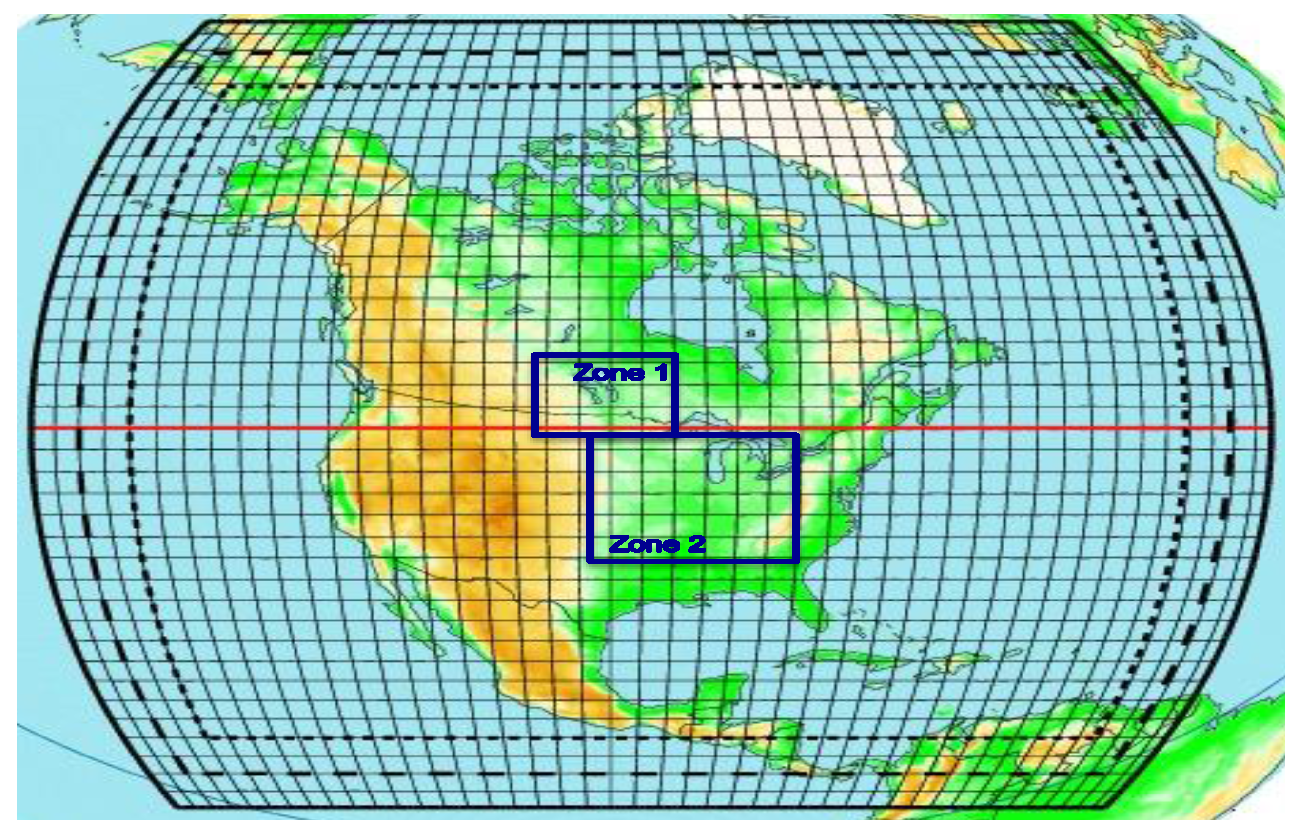
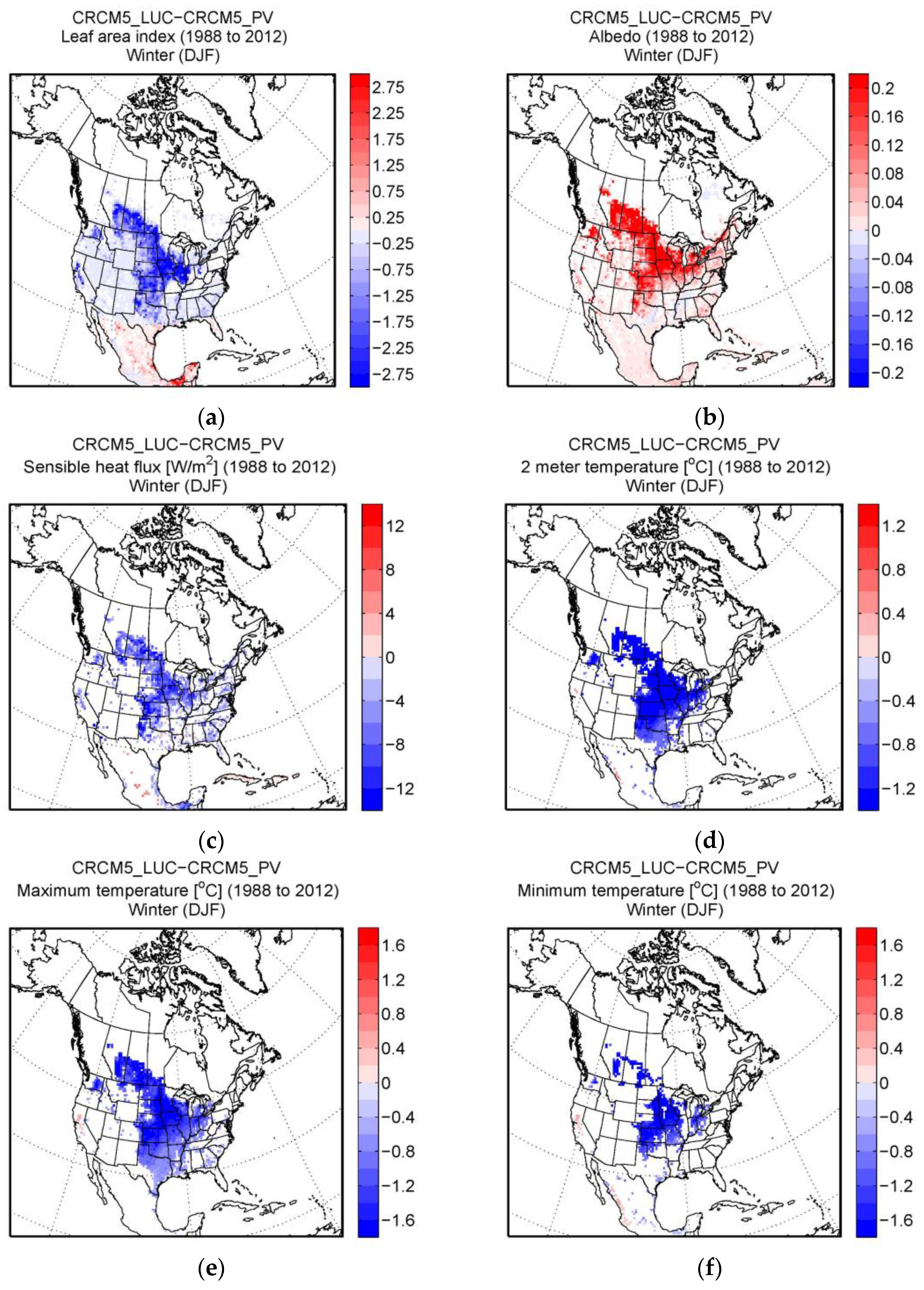
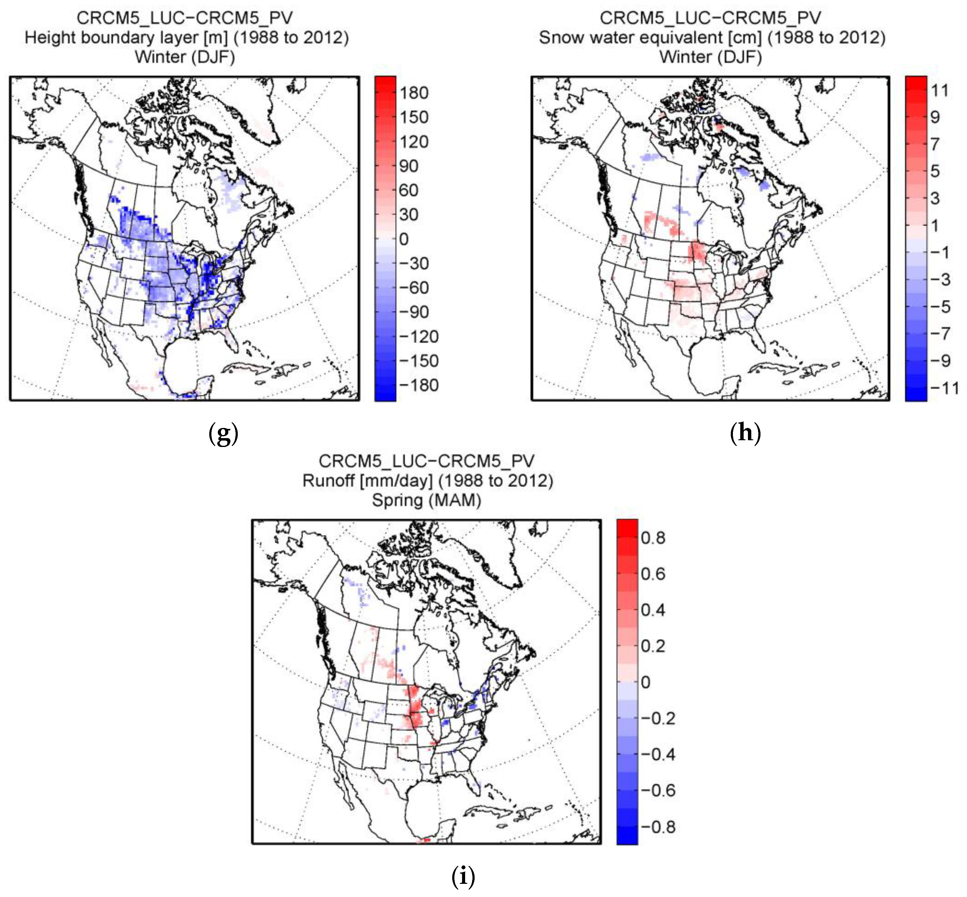
3.1. Spatial Seasonal Analysis

The differences between CRCM5_LUC and CRCM5_PV for the winter and summer months are presented here. References are made to other seasons where required.
Figure 3 shows the differences between CRCM5_LUC and CRCM5_PV for selected surface fluxes and variables for the winter season. Regions with statistically significant differences in leaf area index (LAI) show a dipole pattern, with smaller LAI values in the north and higher values in the south in CRCM5_LUC compared to CRCM5_PV (Figure 3a). This is because, for the northerly regions, the growing season for crops is mostly limited to the spring—early fall periods, leading to zero LAI in winter in CRCM5_LUC. However, for the southern regions (below 30°N), growing season for crops is year round as for broadleaf trees and therefore the LAI values are higher in CRCM5_LUC compared to CRCM5_PV (Figure 3a). Note that for this southern region, fractional areas of both grass and broadleaf were replaced with crops. The above changes to LAI leads to statistically significant differences in albedo between CRCM5_LUC and CRCM5_PV over these LUC regions, particularly for the northern regions (Figure 3b), where albedo values are higher in CRCM5_LUC compared to CRCM5_PV. The regions south of 30°N show slightly higher values of albedo in CRCM5_LUC, despite the higher values of LAI, which is due to relatively drier soil layer at the surface in this simulation. The higher values of albedo in CRCM5_LUC are reflected in the negative differences in sensible heat flux (SHF, Figure 3c) and two meter temperatures (T2M). The differences in T2M is more than 1.4 °C over central Canada and central east US (Figure 3d). The signature of high albedo in CRCM5_LUC can also be seen in the lower values of the daily minimum (TMin) and maximum (TMax) temperatures; the maximum differences between CRCM5_LUC and CRCM5_PV for these temperatures are 1.4 °C and 1.7 °C, respectively (Figure 3e,f). The cooler temperatures in CRCM5_LUC lead to boundary layer heights that are 80 to 200 m lower than that in CRCM5_PV in LUC affected regions. Snow water equivalent presents higher values over central Canada and central east US (Figure 3h), in CRCM5_LUC, which is due to cooler temperatures in this simulation. The higher snow water equivalent values can further increase the albedo values, leading to further cooling and snow water equivalent augmentation through snow-albedo feedback. Furthermore, high values of runoff are noted during spring in CRCM5_LUC, which is consistent with the higher snow water equivalent values in this simulation (Figure 3h,i), as spring runoff is primarily related to snow melt.
The impacts of LUC during the summer season are presented in Figure 4. The differences in LAI between CRCM5_LUC and CRCM5_PV are statistically significant over a larger region, covering regions with important LUC and adjoining areas (Figure 4a). For southerly regions (south of 50°N), the differences are positive, suggesting higher LAI, while for northerly regions (north of 50°N) it is negative, suggesting lower LAI in CRCM5_LUC compared to CRCM5_PV. These negative values for the northern regions are due to shorter growing season of crops, compared to that of grass (which is year round in the model), leading to lower average LAI values. For the northerly regions (north of 50°N) the onset (harvest) happens later (earlier), compared to southern regions. The higher values of LAI for the regions south of 50°N is due to the higher LAI values of crops compared to grass for this region. The regions with significant differences in LAI also show statistically significant differences in albedo (Figure 4b), with albedo being higher in CRCM5_LUC.
The differences in albedo for summer are much smaller than that for winter. The higher values of albedo in CRCM5_LUC for the northern regions is primarily due to the lower LAI values, while for the southern regions, the noted higher values of albedo, despite higher LAI values is partly due to the drier surface soil layers due to increased evaporation. The differences in albedo are reflected in the reduced SHF values over the central and eastern parts of the US in CRCM5_LUC (Figure 4c). The latent heat flux (LHF), on the other hand, appears higher in CRCM5_LUC due to higher LAI for these regions. The lower SHF, and the increased LHF and associated evaporative cooling lead to cooler temperatures in CRCM5_LUC (Figure 4c). This is also reflected in the TMin, TMax and in the soil temperatures (Figure 4f–h).
The comparison of the 10 m wind field between CRCM5_LUC and CRCM5_PV shows statistically significant high wind magnitude values over a small region of northeast US during winter and summer seasons (Figure S1). These high values could be a response to the replacement of broadleaf trees with crops. In central US, statistically significant changes in wind magnitude are observed, where lower values are displayed in both seasons. However, the differences are smaller than 0.5 m/s and 0.25 m/s for summer and winter, respectively (Figure S1). These two small zones, northeast and central US, present changes in the wind field but do not show that LUC impacts circulation and are not indicative of a LUC influenced teleconnection over North America.

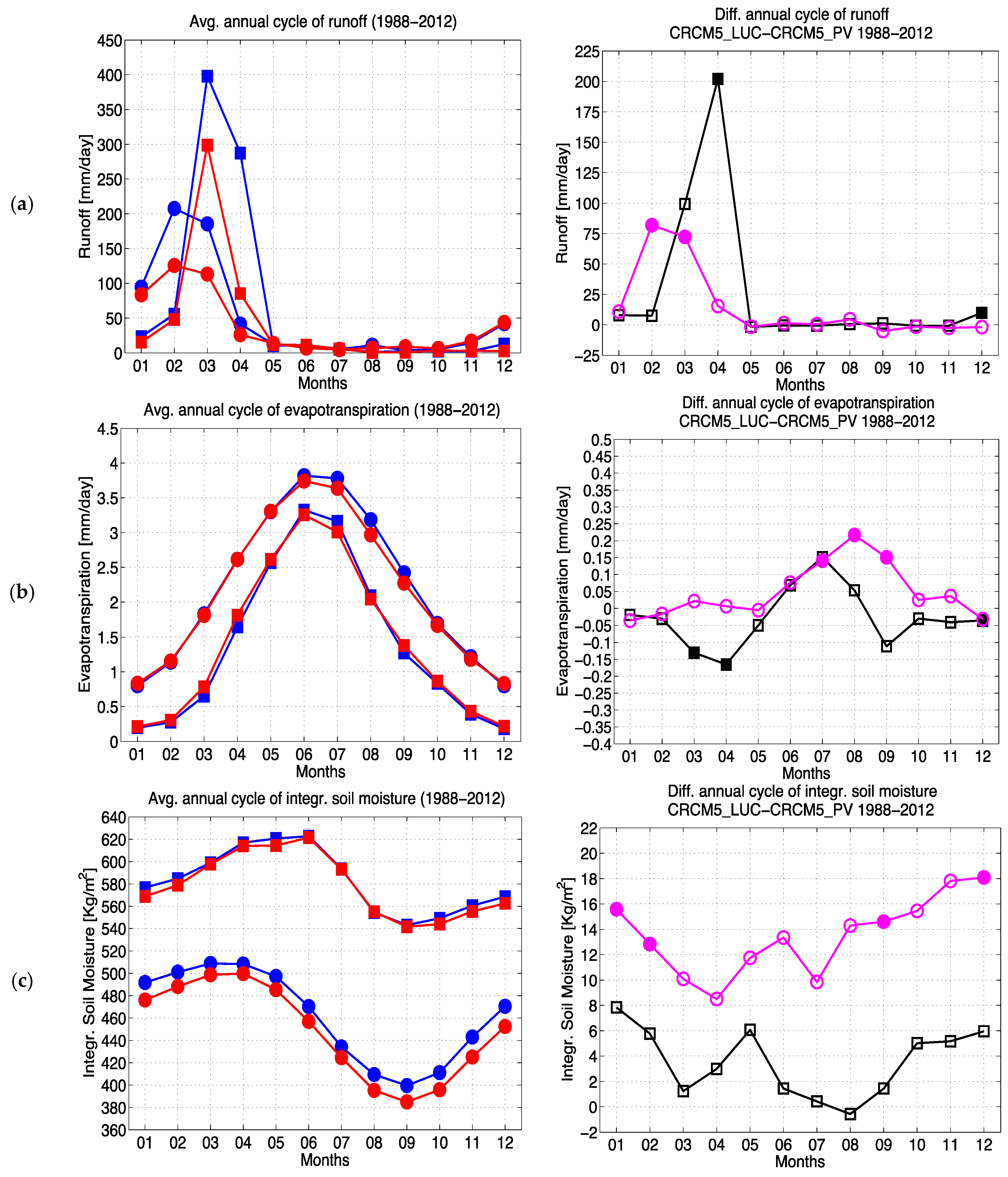
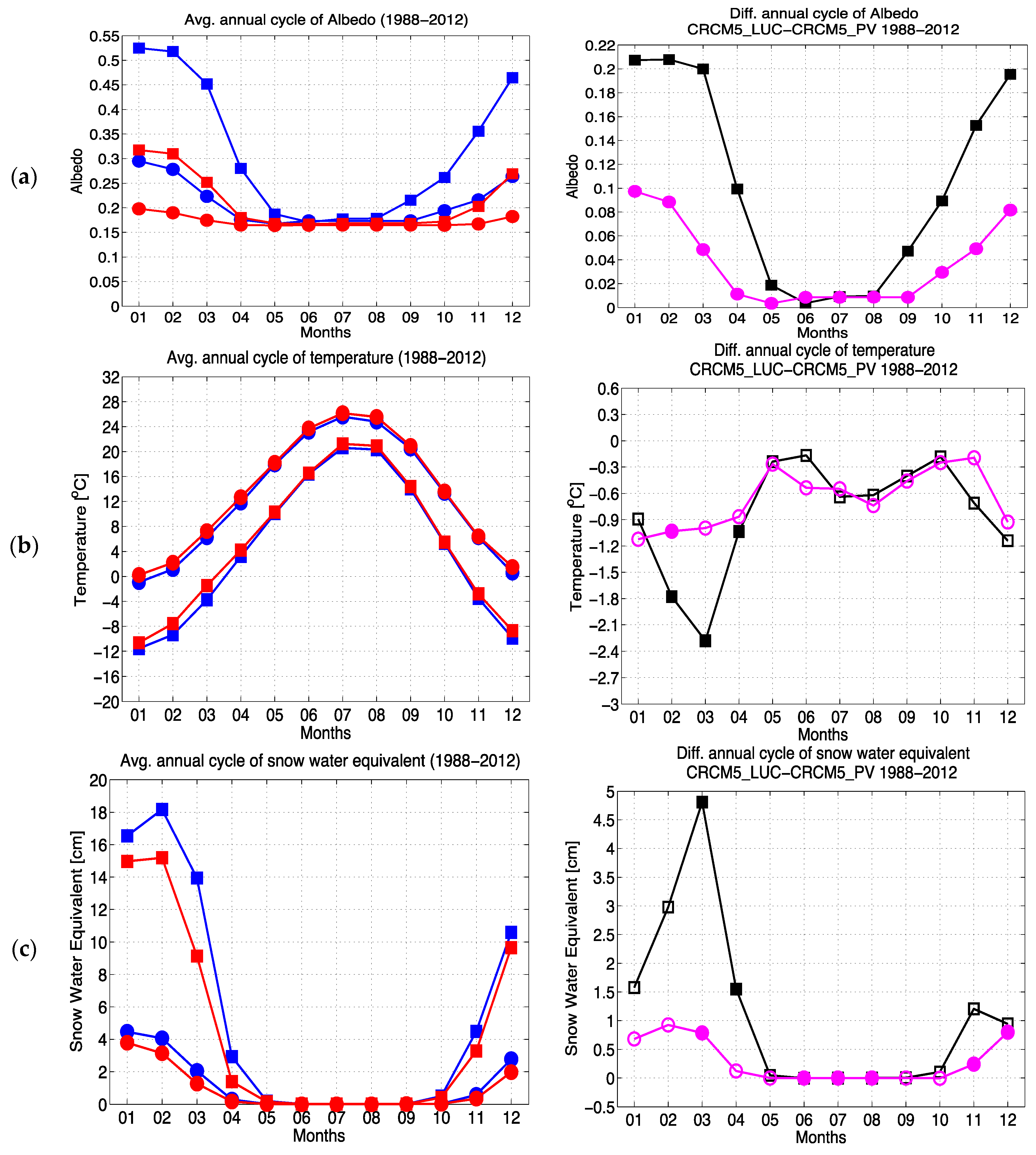
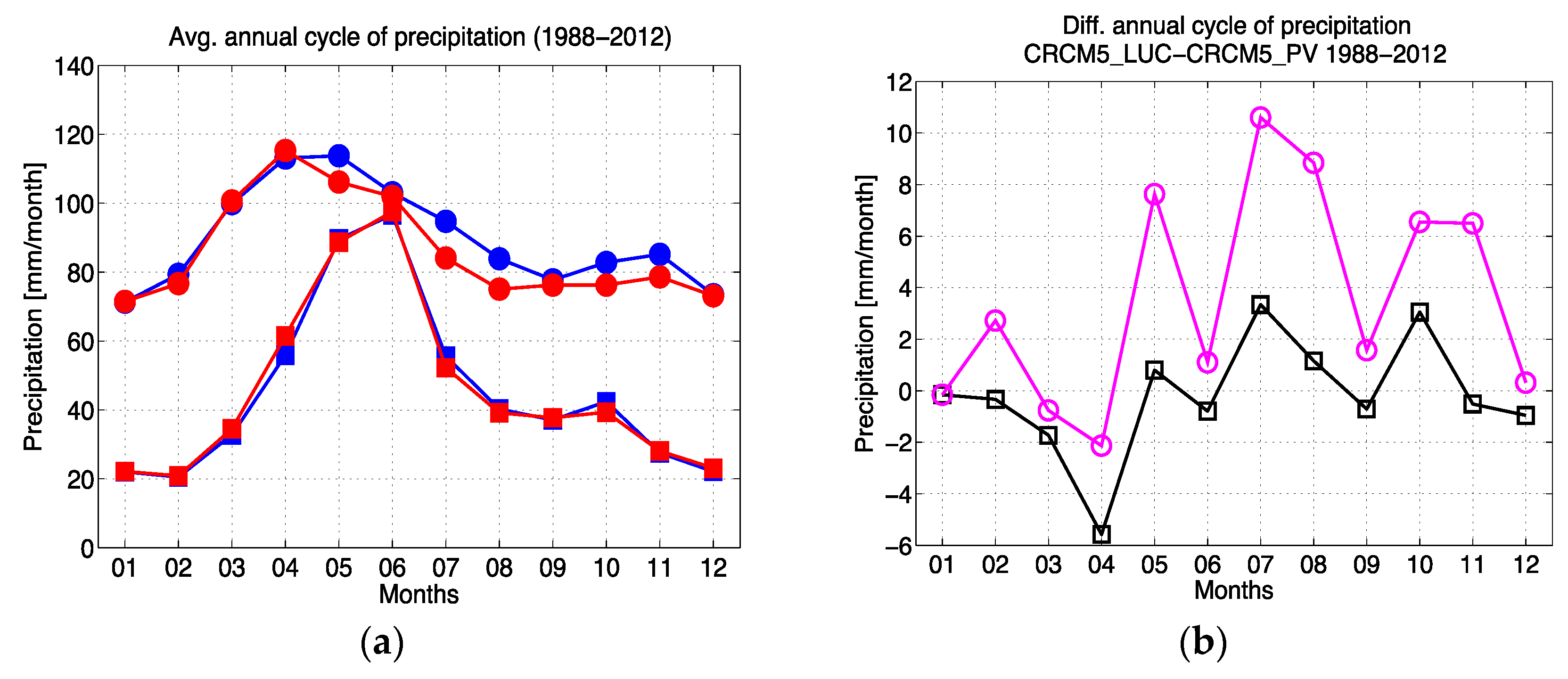
3.2. Analysis of Average Annual Cycles

Results presented above show that the statistically significant differences are mostly collocated with regions of important LUC. Therefore, two regions, zone 1 and zone 2, are defined to look carefully at the differences in the average annual cycles in CRCM5_LUC and CRCM5_PV of selected surface variables. Zone 1 covers 46°–60°N and 94°–114.5°W, and includes central Canada and a small region of northern central US. Zone 2 covers 31°–46°N and 80–103°W, which includes most of the LUC regions in the central to eastern US (Figure 2).
In order to evaluate the LUC effects over these zones, grid points with crops in the CRCM5_LUC simulation in zones 1 and 2 were selected for analyzing the mean annual cycles in both simulations (Figure 5, Figure 6 and Figure 7). The annual cycle of albedo shows high values from January to April and from October to December and low values during the summer months, as expected, due to presence of snow during the late winter to early spring seasons. Both zones present the same tendency, but zone 2 has lower albedo values in winter compared to zone 1, given its southern location (Figure 5a). The annual cycle of the differences between the two simulations, suggest larger differences during the fall to spring periods (Figure 5b). Differences in albedo between the two simulations are larger for zone 1 compared to zone 2, mainly due to the larger differences in snow water equivalent over zone 1 in the two simulations (Figure 5a,c). This relationship reinforces the snow-albedo feedback, as suggested before, during winter months (Figure 5a,c). The higher snow water equivalent values in CRCM5_LUC leads to higher spring peak flows for both zones as shown in Figure 6a. The differences are again larger for zone 1 compared to zone 2 due to its northern location (Figure 5c). Generally higher runoff values are noted for the snowmelt period. The maximum differences in runoff occur at different times for the two zones (Figure 6a). This is due to the fact that snowmelt starts one month earlier in zone 2 because of its geographic location. As for the period of May to October, as discussed earlier, the differences between the two simulations are negligible since runoff is mostly coming from baseflow and surface runoff during precipitation events. Note that no significant differences are noted for precipitation for the two zones. Figure 5b shows the annual cycle of two meter temperature. The comparison between CRCM5_LUC and CRCM5_PV shows that the cooling effect of LUC occurs throughout the year; it is however higher from January to April, with differences higher than 0.9 °C (Figure 5b). The cooling over this period is related to high albedo and possible snow-mediated feedback in CRCM5_LUC as already discussed. On the other hand, the CRCM5_LUC cooling trend observed from May to September is related to higher evapotranspiration values, which is particularly noticeable over zone 2 (Figure 6b). Maximum evapotranspiration is observed in June and July for zones 1 and 2, respectively (Figure 6b). As for the difference between the simulations, CRCM5_LUC for zone 2 shows higher evapotranspiration values over the period of June to November, mostly during the presence of crops over that zone. As for zone 1, the higher evapotranspiration differences are noted from June to August and are smaller than for zone 2, mainly due to shorter growing season in this zone compared to zone 2 (Figure 6b).
The annual cycle of integrated soil moisture shows high values during snowmelt, for both zones (Figure 6c). During the warm months, there is a decreasing tendency in soil moisture as a result of high evapotranspiration (Figure 6b). The integrated soil moisture is generally higher for zone 1, compared to zone 2, despite the higher values of precipitation for zone 2 compared to zone 1 (Figure 7a). The lower values for zone 2 are due to relatively shallow depth to bedrock (Figure not shown). Furthermore, lower values of SWE and therefore snowmelt and high values of evapotranspiration can also be attributed to the lower values for this zone. The differences in soil moisture between CRCM5_LUC and CRCM5_PV are smaller for zone 1 (Figure 6c), compared to zone 2. The differences in precipitation between the two simulations are small (Figure 7b). Precipitation is slightly higher in CRCM5_LUC during the summer months for zone 1 and zone 2 (Figure 7a), but the differences are not statistically significant.

4. Discussion and Conclusions

The biophysical effects of LUC can result in cooling or warming depending on the duration of the growing season, changes in albedo and partitioning of available energy between sensible and latent heat fluxes. The two CRCM5 simulations considered in this study, with and without LUC, suggest significant impacts of LUC on the regional climate of North America. The results show a cooling effect over the LUC regions during winter and summer. The mechanisms leading to this cooling are different for the two periods. The cooling effect of LUC in winter is more than 1.4 °C. This is mainly attributed to the high albedo values in LUC regions, which is further enhanced via snow-albedo feedback, in agreement with Bonan G. [10], Feddeman et al. [17] and Brovkin et al., [16]. As for the summer season, the regions with statistically significant cooling are smaller, with differences in two meter temperature values less than 1.2 °C. The cooling here is primarily due to high (low) latent (sensible) heat flux values. The above impacts of LUC are congruent with the studies of Bonan [19] and Oleson et al. [22] where they report cooler temperatures over the LUC regions of North America in summer season because of high latent heat flux values.
Two zones were analyzed to further understand the influence of LUC, one covering central Canada and the other central east US, using only grid points with crops in the simulation with LUC. Analysis of the seasonal cycles for both simulations suggests that the cooling effect of LUC is present year round. The impacts of LUC on evapotranspiration and soil moisture are also year round. However, the impact on runoff is mostly restricted to snowmelt season. It should be noted that the precipitation differences are not statistically significant. This could be due to the weak soil moisture-precipitation coupling over the Great Plains in CRCM5 as discussed in Diro et al. [57]. Furthermore, the absence of irrigation in CRCM5_LUC, could also contribute to the non-significant differences in precipitation between the two simulations.
In this study, only croplands were used to represent human activity over North America and the biophysical effects of this LUC were evaluated. The influence of irrigation over croplands is not included, but it would be important to implement it in future regional climate simulations. Studies, however, have been done using GCMs that include irrigation. For example, Haddeland et al. [58] in their study used an irrigation scheme over Colorado and Mekong River basins and found that latent heat flux increases along with a decreases of temperature, over these areas. This was identified over large fraction of grid cells where the irrigation was implemented. Lo and Famiglietti [59], in their study using a regional climate model with irrigation over the central valley of California, showed that irrigation leads to an increase in evapotranspiration leading to net land surface cooling. Another important influence was an increase in precipitation, mainly in summer, enhancing the monsoon rainfall over the southwest US.
It must also be noted that sub-grid lakes and wetlands were not considered in this study. These should also be included in futures studies. Furthermore, future studies should also take into account pastures, urban areas and disturbances such as fire. It is also important to consider LUC in transient climate change simulations with regional climate models. Currently, many regional climate models do not include this. Studies with global climate models have shown that urbanization leads to warming at regional and local scales, pastures lead to cooling over temperate zones and fires lead to decreases in precipitation due to reduced evapotranspiration [8,60,61]. CRCM5 transient climate change simulations, including land use change will be performed in the near future to investigate the biophysical effects of LUC on projected changes to the surface climate and hydrology over North America.

Supplementary Materials

The following are available online at https://www.mdpi.com/2073-4433/7/3/34/s1, Figure S1: Seasonal average wind at 10 m for 1988–2012 period for (a) winter and (b) summer seasons. Differences between CRCM5_LUC and CRCM5_PV for 1988–2012 period for (c) winter and (d) summer seasons. Colour shading indicates grid points with statistically significant differences at 0.05 level.

Acknowledgments

This work was supported by the Natural Sciences and Engineering Research Council of Canada Discovery Grants (NSERC-DG) and the Canada Research Chairs programs. Arlette Chacón was the recipient of a NSERC-CREATE—Training Program in Climate Sciences graduate fellowship. Computational resources were provided by Centre pour l’Étude et la Simulation du Climat à l’Échelle Régional (ESCER) at Université du Québec à Montréal (UQAM) and Calcul Québec, an organization of Québec Universities brought together by Advanced Research Computing (ARC).

Author Contributions

The authors conceived and designed the experiment for this study. Arlette Chacón did the model experiments, analysed model data and prepared the first version of the manuscript. Laxmi Sushama and Hugo Beltrami supervised the analysis and contributed to the writing and revision of the manuscript.

Conflicts of Interest

The authors declare no conflict of interest.

References

  1. Mahmood, R.; Quintanar, A.I.; Conner, G.; Leeper, R.; Dobler, S.; Pielke, R.A.; Beltran-Przekurat, A.; Hubbard, K.G.; Niyogi, D.; Bonan, G.; et al. Impacts of land use/land cover change on climate and future research priorities. Bull. Am. Meteorol. Soc. 2010, 91, 37–46. [Google Scholar] [CrossRef]
  2. Pachauri, R.K.; Allen, M.R.; Barros, V.R.; Broome, J.; Cramer, W.; Christ, R.; Church, J.A.; Clarke, L.; Dahe, Q.; Dasgupta, P.; et al. Climate Change 2014: Synthesis Report. Contribution of Working Groups I, II and III to the Fifth Assessment Report of the Intergovernmental Panel on Climate Change; IPCC: Geneva, Switzerland, 2014.
  3. DeFries, R.S.; Foley, J.A.; Asner, G.P. Land-use choices: Balancing human needs and ecosystem function. Front. Ecol. Environ. 2004, 2, 249–257. [Google Scholar] [CrossRef]
  4. Foley, J.A.; Defries, R.; Asner, G.P.; Barford, C.; Bonan, G.; Carpenter, S.R.; Chapin, F.S.; Coe, M.T.; Daily, G.C.; Gibbs, H.K.; et al. Global consequences of land use. Science 2005, 309, 570–574. [Google Scholar] [CrossRef] [PubMed]
  5. Ramankutty, N.; Evan, A.T.; Monfreda, C.; Foley, J.A. Farming the planet: 1. Geographic distribution of global agricultural lands in the year 2000. Glob. Biogeochem. Cycles 2008, 22. [Google Scholar] [CrossRef]
  6. Goldewijk, K.K. Estimating global land use change over the past 300 years: The hyde database. Glob. Biogeochem. Cycles 2001, 15, 417–433. [Google Scholar] [CrossRef]
  7. Georgescu, M.; Lobell, D.B.; Field, C.B. Direct climate effects of perennial bioenergy crops in the united states. Proc. Natl. Acad. Sci. USA 2011, 108, 4307–4312. [Google Scholar] [CrossRef] [PubMed]
  8. Boysen, L.R.; Brovkin, V.; Arora, V.K.; Cadule, P.; de Noblet-Ducoudré, N.; Kato, E.; Pongratz, J.; Gayler, V. Global and regional effects of land-use change on climate in 21st century simulations with interactive carbon cycle. Earth Syst. Dyn. 2014, 5, 309–319. [Google Scholar] [CrossRef]
  9. Friedlingstein, P.; Dufresne, J.-L.; Cox, P.; Rayner, P. How positive is the feedback between climate change and the carbon cycle? Tellus B 2003, 55, 692–700. [Google Scholar] [CrossRef]
  10. Bonan, G.B. Forests and climate change: Forcings, feedbacks, and the climate benefits of forests. Science 2008, 320, 1444–1449. [Google Scholar] [CrossRef] [PubMed]
  11. Davin, E.L.; de Noblet-Ducoudré, N.; Friedlingstein, P. Impact of land cover change on surface climate: Relevance of the radiative forcing concept. Geophys. Res. Lett. 2007, 34. [Google Scholar] [CrossRef]
  12. De Noblet-Ducoudré, N.; Boisier, J.-P.; Pitman, A.; Bonan, G.B.; Brovkin, V.; Cruz, F.; Delire, C.; Gayler, V.; van den Hurk, B.J.J.M.; Lawrence, P.J.; et al. Determining robust impacts of land-use-induced land cover changes on surface climate over North America and Eurasia: Results from the first set of lucid experiments. J. Clim. 2012, 25, 3261–3281. [Google Scholar] [CrossRef]
  13. Pitman, A.J.; de Noblet-Ducoudré, N.; Cruz, F.T.; Davin, E.L.; Bonan, G.B.; Brovkin, V.; Claussen, M.; Delire, C.; Ganzeveld, L.; Gayler, V.; et al. Uncertainties in climate responses to past land cover change: First results from the lucid intercomparison study. Geophys. Res. Lett. 2009, 36. [Google Scholar] [CrossRef]
  14. Mahmood, R.; Pielke, R.A.; Hubbard, K.G.; Niyogi, D.; Dirmeyer, P.A.; McAlpine, C.; Carleton, A.M.; Hale, R.; Gameda, S.; Beltrán-Przekurat, A.; et al. Land cover changes and their biogeophysical effects on climate. Int. J. Climatol. 2014, 34, 929–953. [Google Scholar] [CrossRef]
  15. Brovkin, V.; Claussen, M.; Driesschaert, E.; Fichefet, T.; Kicklighter, D.; Loutre, M.F.; Matthews, H.D.; Ramankutty, N.; Schaeffer, M.; Sokolov, A. Biogeophysical effects of historical land cover changes simulated by six earth system models of intermediate complexity. Clim. Dyn. 2006, 26, 587–600. [Google Scholar] [CrossRef]
  16. Brovkin, V.; Ganopolski, A.; Claussen, M.; Kubatzki, C.; Petoukhov, V. Modelling climate response to historical land cover change. Glob. Ecol. Biogeogr. 1999, 8, 509–517. [Google Scholar] [CrossRef]
  17. Feddema, J.; Oleson, K.; Bonan, G.; Mearns, L.; Washington, W.; Meehl, G.; Nychka, D. A comparison of a GCM response to historical anthropogenic land cover change and model sensitivity to uncertainty in present-day land cover representations. Clim. Dyn. 2005, 25, 581–609. [Google Scholar] [CrossRef]
  18. Lawrence, P.J.; Chase, T.N. Investigating the climate impacts of global land cover change in the community climate system model. Int. J. Climatol. 2010, 30, 2066–2087. [Google Scholar] [CrossRef]
  19. Bonan, G.B. Effects of land use on the climate of the United States. Clim. Chang. 1997, 37, 449–486. [Google Scholar] [CrossRef]
  20. Findell, K.L.; Shevliakova, E.; Milly, P.C.D.; Stouffer, R.J. Modeled impact of anthropogenic land cover change on climate. J. Clim. 2007, 20, 3621–3634. [Google Scholar] [CrossRef]
  21. Pielke, R.A. Influence of the spatial distribution of vegetation and soils on the prediction of cumulus convective rainfall. Rev. Geophys. 2001, 39, 151. [Google Scholar] [CrossRef]
  22. Oleson, K.W.; Bonan, G.B.; Levis, S.; Vertenstein, M. Effects of land use change on North American climate: Impact of surface datasets and model biogeophysics. Clim. Dyn. 2004, 23, 117–132. [Google Scholar] [CrossRef]
  23. Hua, W.-J.; Chen, H.-S. Impacts of regional-scale land use/land cover change on diurnal temperature range. Adv. Clim. Chang. Res. 2013, 4, 166–172. [Google Scholar]
  24. Pielke, R.A.; Pitman, A.; Niyogi, D.; Mahmood, R.; McAlpine, C.; Hossain, F.; Goldewijk, K.K.; Nair, U.; Betts, R.; Fall, S.; et al. Land use/land cover changes and climate: Modeling analysis and observational evidence. Wiley Interdiscip. Rev.: Clim. Chang. 2011, 2, 828–850. [Google Scholar] [CrossRef]
  25. Gao, X.; Zhang, D.; Chen, Z.; Pal, J.S.; Giorgi, F. Land use effects on climate in China as simulated by a regional climate model. Sci. China Ser. D: Earth Sci. 2007, 50, 620–628. [Google Scholar] [CrossRef]
  26. Nogherotto, R.; Coppola, E.; Giorgi, F.; Mariotti, L. Impact of congo basin deforestation on the African monsoon. Atmos. Sci. Lett. 2013, 14, 45–51. [Google Scholar] [CrossRef]
  27. Akkermans, T.; Thiery, W.; Van Lipzig, N.P.M. The regional climate impact of a realistic future deforestation scenario in the Congo Basin. J. Clim. 2014, 27, 2714–2734. [Google Scholar] [CrossRef]
  28. Lawrence, D.; Vandecar, K. Effects of tropical deforestation on climate and agriculture. Nat. Clim. Chang. 2014, 5, 27–36. [Google Scholar] [CrossRef]
  29. Martynov, A.; Laprise, R.; Sushama, L.; Winger, K.; Šeparović, L.; Dugas, B. Reanalysis-driven climate simulation over cordex North America domain using the Canadian regional climate model, version 5: Model performance evaluation. Clim. Dyn. 2013, 41, 2973–3005. [Google Scholar] [CrossRef] [Green Version]
  30. Côté, J.; Gravel, S.; Méthot, A.; Patoine, A.; Roch, M.; Staniforth, A. The operational CMC–MRB global environmental multiscale (GEM) model. Part 1: Design considerations and formulation. Mon. Weather Rev. 1998, 126, 1373–1395. [Google Scholar] [CrossRef]
  31. Yeh, K.-S.; Côté, J.; Gravel, S.; Méthot, A.; Patoine, A.; Roch, M.; Staniforth, A. The CMC–MRB global environmental multiscale (GEM) model. Part III: Nonhydrostatic formulation. Mon. Weather Rev. 2002, 130, 339–356. [Google Scholar] [CrossRef]
  32. Laprise, R. The euler equation of motion with hydrostatic pressure as independent coordinate. Mon. Weather Rev. 1992, 120, 197–207. [Google Scholar] [CrossRef]
  33. Kain, J.; Fritsch, M. A one-dimensional entraining/detraining plume model and application in convective parameterization. J. Atmos. Sci. 1990, 47, 2784–2802. [Google Scholar] [CrossRef]
  34. Kuo, H.L. On formation and intensification of tropical cyclones through latent heat release by cumulus convection. J. Atmos. Sci. 1965, 22, 40–63. [Google Scholar] [CrossRef]
  35. Bélair, S.; Mailhot, J.; Girard, C.; Vaillancourt, P. Boundary layer and shallow cumulus clouds in a medium-range forecast of a large-scale weather system. Mon. Weather Rev. 2005, 133, 1938–1960. [Google Scholar] [CrossRef]
  36. Sundqvist, H.; Berge, E.; Kristjansson, J.E. Condensation and cloud parameterization studies with a mesoscale numerical weather prediction model. Mon. Weather Rev. 1989, 117, 1641–1657. [Google Scholar] [CrossRef]
  37. Li, J.; Barker, H.W. A radiation algorithm with correlated-k distribution. Part 1: Local thermal equilibrium. J. Atmos. Sci. 2005, 62, 286–309. [Google Scholar] [CrossRef]
  38. McFarlane, N.A. The effect of orographically excited gravity-wave drag on the circulation of the lower stratosphere and troposphere. J. Atmos. Sci. 1987, 44, 1175–1800. [Google Scholar] [CrossRef]
  39. Zadra, A.; Roch, M.; Laroche, S.; Charron, M. The subgrid-scale orographic blocking parametrization of the GEM model. Atmos.-Ocean 2003, 41, 155–170. [Google Scholar] [CrossRef]
  40. Benoit, R.; Côté, J.; Mailhot, J. Inclusion of a tke boundary layer parameterization in the canadian regional finite-element model. Mon. Weather. Rev. 1989, 117, 1726–1750. [Google Scholar] [CrossRef]
  41. Delage, Y.; Girard, C. Stability functions correct at the free convection limit and consistent for both the surface and ekman layers. Bound. Layer Meteor. 1992, 58, 19–31. [Google Scholar] [CrossRef]
  42. Delage, Y. Parameterising sub-grid scale vertical transport in atmospheric models under statically stable conditions. Bound.-Layer Meteor. 1997, 82, 23–48. [Google Scholar] [CrossRef]
  43. Verseghy, D.L. Class-A Canadian land surface scheme for GCMs. I. Soil model. Int. J. Climatol. 1991, 11, 111–133. [Google Scholar] [CrossRef]
  44. Verseghy, D.L.; McFarlane, N.A.; Lazare, M. Class-A Canadian land surface scheme for GCMs. Vegetation model and coupled run. Int. J. Climatol. 1993, 13, 347–370. [Google Scholar] [CrossRef]
  45. Ramankutty, N.; Foley, J.A. Estimating historical changes in global land cover: Croplands from 1700 to 1992. Glob. Biogeochem. Cycles 1999, 13, 997–1027. [Google Scholar] [CrossRef]
  46. Loveland, T.R.; Belward, A.S. The IGBP-DIS global 1km land cover data set, discover: First results. Int. J. Remote Sens. 1997, 18, 3289–3295. [Google Scholar] [CrossRef]
  47. Haxeltine, A.; Prentice, I.C. Biome3: An equilibrium terrestrial biosphere model based on ecophysiological constraints, resource availability, and competition among plant functional types. Glob. Biogeochem. Cycles 1996, 10, 693–709. [Google Scholar] [CrossRef]
  48. Friedl, M.A.; McIver, D.K.; Hodges, J.C.F.; Zhang, X.Y.; Muchoney, D.; Strahler, A.H.; Woodcock, C.E.; Gopal, S.; Schneider, A.; Cooper, A.; et al. Global land cover mapping from modis: Algorithms and early results. Remote Sens. Environ. 2002, 83, 287–302. [Google Scholar] [CrossRef]
  49. Bartholomé, E.; Belward, A.S. GLC2000: A new approach to global land cover mapping from earth observation data. Int. J. Remote Sens. 2005, 26, 1959–1977. [Google Scholar] [CrossRef]
  50. Dee, D.P.; Uppala, S.M.; Simmons, A.J.; Berrisford, P.; Poli, P.; Kobayashi, S.; Andrae, U.; Balmaseda, M.A.; Balsamo, G.; Bauer, P.; et al. The Era-Interim reanalysis: Configuration and performance of the data assimilation system. Quarterly J. R. Meteorol. Soc. 2011, 137, 553–597. [Google Scholar] [CrossRef]
  51. Verseghy, D.L. Class—The canadian land surface scheme. Int. J. Clim. 1991, 12. [Google Scholar] [CrossRef]
  52. Henderson-Sellers, A.; Pitman, A.; Love, P.; Irannejad, P.; Chen, T. The project for intercomparison of land surface parameterization schemes (PILPS): Phases 2 and 3. Bull. Am. Meteorol. Soc. 1995, 76, 489–503. [Google Scholar] [CrossRef]
  53. Henderson-Sellers, A.; McGuffie, A.K.; Pitman, A.J. The project for intercomparison of land-surface parameterization schemes (PILPS): 1992 to 1995. Clim. Dyn. 1996, 12, 849–859. [Google Scholar] [CrossRef]
  54. Pitman, A.; Henderson-Sellers, A. Recent progress and results from the project for the intercomparison of landsurface parameterization schemes. J. Hydrol. 1998, 212, 128–135. [Google Scholar] [CrossRef]
  55. Langlois, A.; Bergeron, J.; Brown, R.; Royer, A.; Harvey, R.; Roy, A.; Wang, L.; Thériault, N. Evaluation of class 2.7 and 3.5 simulations of snow properties from the Canadian regional climate model (CRCM4) over Québec, Canada*. J. Hydrometeorol. 2014, 15, 1325–1343. [Google Scholar] [CrossRef]
  56. Haghnegahdar, A.; Tolson, B.A.; Davison, B.; Seglenieks, F.R.; Klyszejko, E.; Soulis, E.D.; Fortin, V.; Matott, L.S. Calibrating environment Canada′s mesh modelling system over the great lakes basin. Atmos.-Ocean. 2014, 52, 281–293. [Google Scholar] [CrossRef]
  57. Diro, G.T.; Sushama, L.; Martynov, A.; Jeong, D.I.; Verseghy, D.; Winger, K. Land-atmosphere coupling over north america in CRCM5. J. Geophys. Res.: Atmos. 2014, 119, 11,955–11,972. [Google Scholar] [CrossRef]
  58. Haddeland, I.; Lettenmaier, D.P.; Skaugen, T. Effects of irrigation on the water and energy balances of the colorado and mekong river basins. J. Hydrol. 2006, 324, 210–223. [Google Scholar] [CrossRef]
  59. Lo, M.-H.; Famiglietti, J.S. Irrigation in California′s central valley strengthens the southwestern U.S. Water cycle. Geophys. Res. Lett. 2013, 40, 301–306. [Google Scholar] [CrossRef]
  60. He, J.F.; Liu, J.Y.; Zhuang, D.F.; Zhang, W.; Liu, M.L. Assessing the effect of land use/land cover change on the change of urban heat island intensity. Theor. Appl. Climatol. 2007, 90, 217–226. [Google Scholar] [CrossRef]
  61. Cochrane, M.A.; Laurance, W.F. Synergisms among fire, land use and climate change in the Amazon. AMBIO: A J. Hum. Environ. 2008, 38, 522–527. [Google Scholar] [CrossRef]
Figure 1. Simulation domain: 220 × 200 points grid at 0.44° horizontal resolution (only every 5th grid point is displayed). The dashed and dotted lines represent the “halo” and sponge zones, respectively. The remaining is the free domain of 160 × 180 grid points. The two blue boxes represent regions considered for analyzing the seasonal cycle (zone 1 covers 46°–60°N and 93°–121°W and zone 2 covers 31°–46°N and 80–108°W).
Atmosphere 07 00034 g001
Figure 2. (a) Needleleaf; (b) broadleaf; (c) crops; and (d) grass fractional areas for CRCM5 simulations with: potential vegetation dataset called CRCM5_PV (left) and present-land use dataset called CRCM5_LUC (right).
Atmosphere 07 00034 g002aAtmosphere 07 00034 g002b
Figure 3. Differences between CRCM_LUC and CRCM_PV, for winter, for: (a) leaf area index; (b) albedo; (c) sensible heat flux; (d) maximum temperature; (e) minimum temperature; (f) two meter temperature; (g) height of the boundary layer; (h) snow depth; and (i) runoff. Values are shown only for grid points where the differences are statistically significant at 95% confidence level.
Atmosphere 07 00034 g003aAtmosphere 07 00034 g003b
Figure 4. Differences between CRCM_LUC and CRCM_PV, for summer season, for: (a) leaf area index; (b) albedo; (c) sensible heat flux; (d) latent heat flux; (e) two meter temperature; (f) maximum temperature; (g) minimum temperature; and (h) soil temperature. Values are shown only for grid points where the differences are statistically significant at 95% confidence level.
Atmosphere 07 00034 g004aAtmosphere 07 00034 g004b
Figure 5. (Left) Average annual cycle for the 1988–2012 period for: (a) albedo; (b) two meter temperature; and (c) snow water equivalent (Red: CRCM5_PV; Blue: CRCM5_LUC; squares and circles are used for zone 1 and zone 2, respectively). (Right) Difference between CRCM5_LUC and CRCM5_PV for: (a) albedo; (b) two meter temperature; and (c) snow water equivalent (Black: zone 1; Magenta: zone 2; filled squares are circles are used for differences that are statistically significant at 95% confidence level).
Atmosphere 07 00034 g005
Figure 6. (Left) Average annual cycle for the 1988–2012 period for: (a) runoff; (b) evapotranspiration; and (c) integrated soil moisture (Red: CRCM5_PV; Blue: CRCM5_LUC; squares and circles are used for zone 1 and zone 2, respectively). (Right) Difference between CRCM5_LUC and CRCM5_PV for: (a) runoff; (b) evapotranspiration; and (c) integrated soil moisture (Black: zone 1; Magenta: zone 2; filled squares are circles are used for differences that are statistically significant at 95% confidence level).
Atmosphere 07 00034 g006
Figure 7. (a) Average annual cycle for the 1988–2012 period for precipitation (Red: CRCM5_PV; Blue: CRCM5_LUC; squares and circles are used for zone 1 and zone 2, respectively). (b) Difference between CRCM5_LUC and CRCM5_PV for precipitation (Black: zone 1; Magenta: zone 2; filled squares are circles are used for differences that are statistically significant at 95% confidence level).
Atmosphere 07 00034 g007

