
Source Localization in the Duct Environment with the Adjoint of the PE Propagation Model


Abstract
:1. Introduction
2. Propagation Model
3. Adjoint Operator
4. Numerical Experiments and Analysis

| Height (m) | Refractivity (M-units) |
|---|---|
| 0 | 330 |
| 50 | 320 |
| 1050 | 438 |
| Frequency (MHz) | Beamwidth (°) | Elevation (°) | Height (m) |
|---|---|---|---|
| 5000 | 0.4 | 0 | 30 |
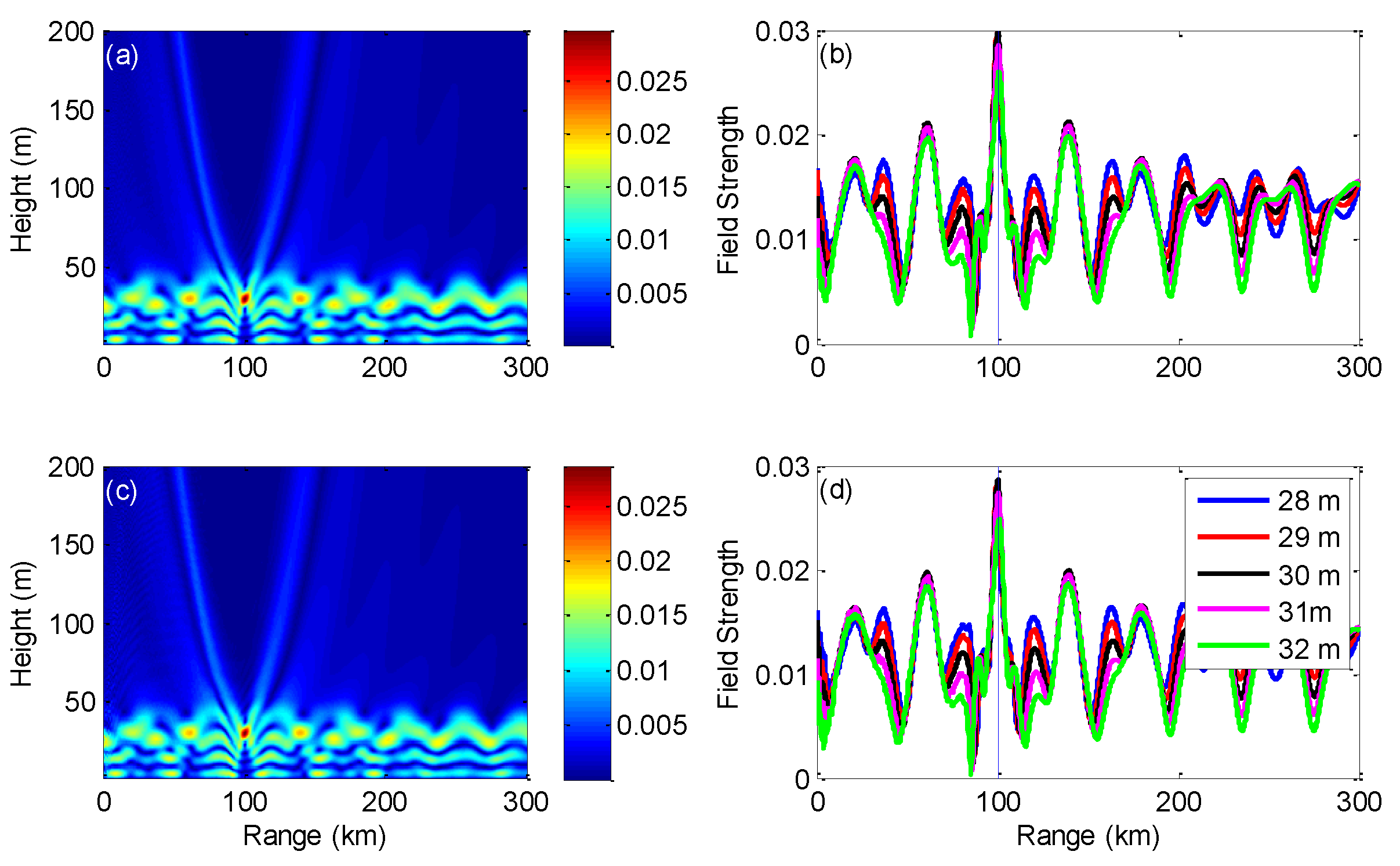
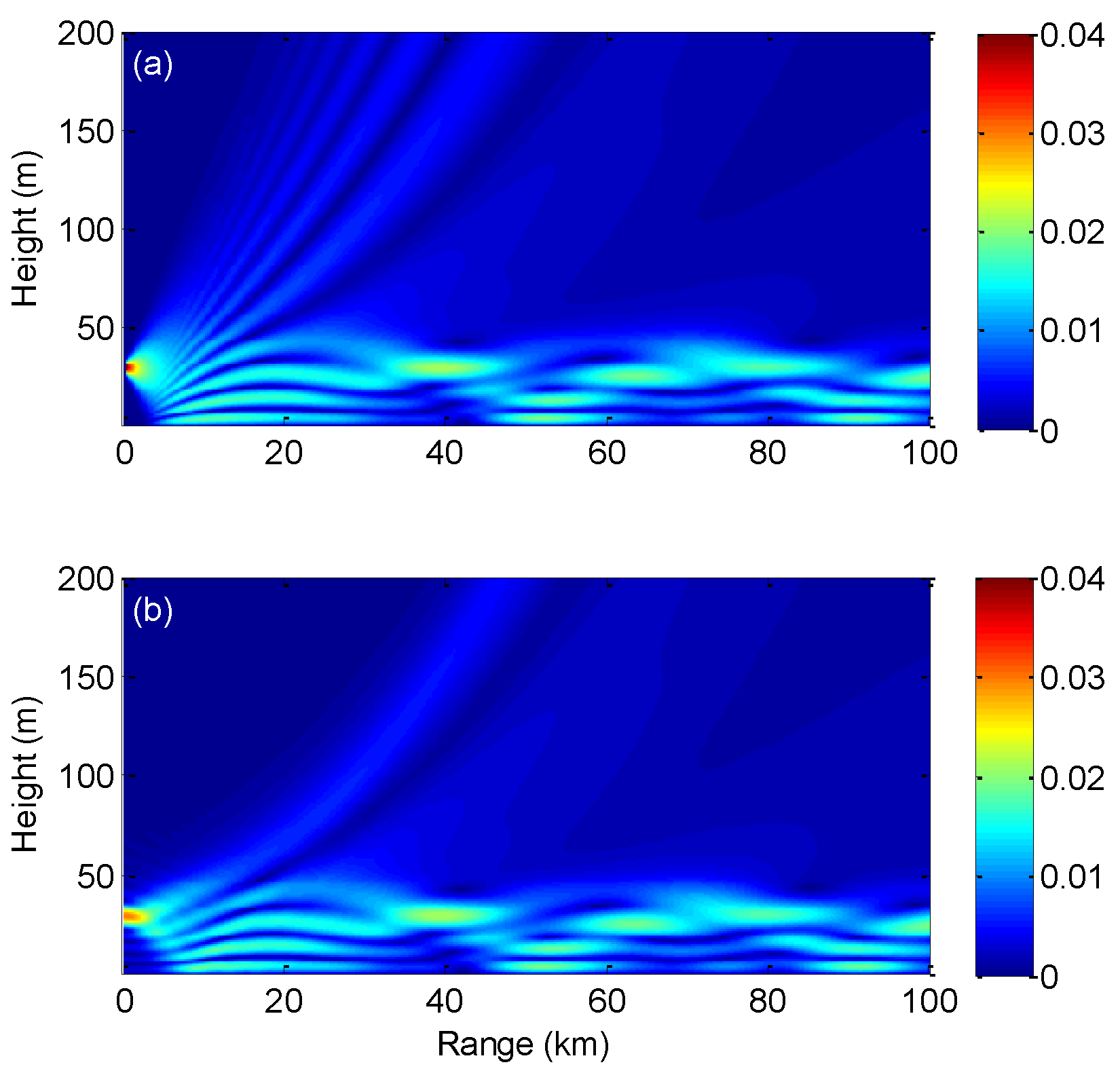
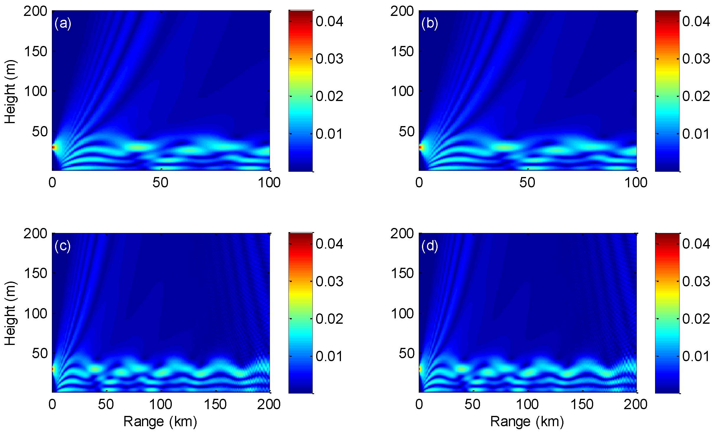
4.1. Propagation Fields Reconstruction
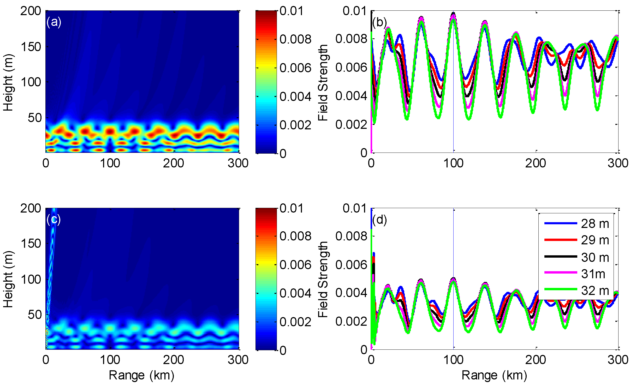
4.2. Noise Influence


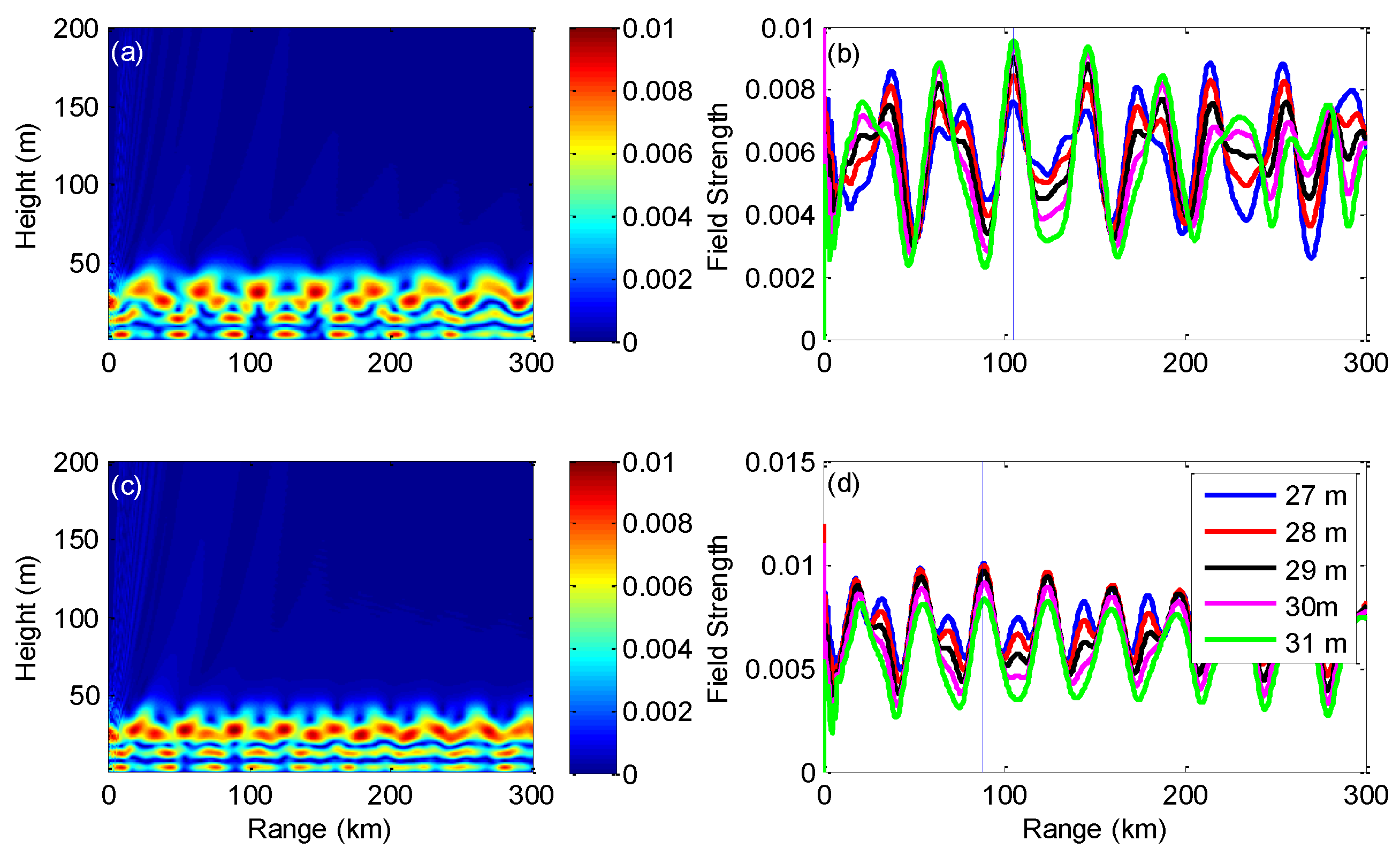
4.3. Receiver Geometry Influence

5. Conclusions
Acknowledgments
Conflicts of Interest
Appendix: Propagation Fields Reconstruction without Filtering Window
References
- Cheung, K.W.; So, H.C. A multidimensional scaling framework for mobile location using time-of-arrival measurements. IEEE Trans. Signal Process. 2005, 53, 460–470. [Google Scholar]
- Sayed, A.H.; Tarighat, A.; Khajehnouri, N. Network-based wireless location: Challenges faced in developing techniques for accurate wireless location information. IEEE Signal Process. Mag. 2015, 22, 24–40. [Google Scholar] [CrossRef]
- Beck, A.; Stoica, P.; Li, J. Exact and approximate solutions of source localization problems. IEEE Trans. Signal Process. 2008, 56, 1770–1778. [Google Scholar] [CrossRef]
- Gingras, D.F.; Gerstoft, P.; Gerr, N.L. Electromagnetic matched field processing: Basic concepts and tropospheric simulations. IEEE Trans. Antennas Propag. 1997, 45, 1536–1545. [Google Scholar] [CrossRef]
- Spencer, T.A.; Walker, R.A.; Hawkes, R.M. Inverse diffraction parabolic wave equation localization system (IDPELS). J. Glob. Position. Syst. 2005, 4, 245–247. [Google Scholar] [CrossRef]
- Zhao, X. Evaporation duct height estimation and source localization from field measurements at an array of radio receivers. IEEE Trans. Antennas Propag. 2012, 60, 1020–1025. [Google Scholar] [CrossRef]
- Dockery, G.D. Modeling electromagnetic wave propagation in the troposphere using the parabolic equation. IEEE Trans. Antennas Propag. 1988, 36, 1464–1470. [Google Scholar] [CrossRef]
- Kuttler, J.R.; Dockery, G.D. Theoretical description of the parabolic approximation/Fourier split-step method of representing electromagnetic propagation in the troposphere. Radio Sci. 1991, 26, 381–393. [Google Scholar] [CrossRef]
- Craig, K.H.; Levy, M.F. Parabolic equation modeling of the effects of multipath and ducting on radar systems. IEE Proc. F Radar Signal Process 1991, 138, 153–162. [Google Scholar] [CrossRef]
- Barrios, A.E. Parabolic equation modeling in horizontally inhomogeneous environments. IEEE Trans. Antennas Propag. 1992, 40, 791–797. [Google Scholar] [CrossRef]
- Barrios, A.E. A terrain parabolic equation model for propagation in the troposphere. IEEE Trans. Antennas Propag. 1994, 42, 90–98. [Google Scholar] [CrossRef]
- Valtr, P.; Pechac, P.; Kvicera, V.; Grabner, M. A terrestrial multiple-receiver radio link experiment at 10.7 GHz—Comparisons of results with parabolic equation calculations. Radioengineering 2010, 19, 117–121. [Google Scholar]
- Errico, R.M. What is an adjoint model? Bull. Am. Meteorol. Soc. 1997, 78, 2577–2591. [Google Scholar] [CrossRef]
- Giering, R.; Kaminski, T. Recipes for adjoint code construction. ACM Trans. Math. Softw. 1998, 24, 437–474. [Google Scholar] [CrossRef]
- Zhou, Z.; Li, Y.; Shi, H.; Ma, N.; Shen, J. Pan-sharpening: A fast variational fusion approach. Sci. China Inf. Sci. 2012, 55, 615–625. [Google Scholar] [CrossRef]
- Zhou, Z.; Ma, N.; Li, Y.; Yang, P.; Zhang, P.; Li, Y. Variational PCA fusion for Pan-sharpening very high resolution imagery. Sci. China Inf. Sci. 2014, 57, 1–10. [Google Scholar] [CrossRef]
- Koziel, S.; Ogurtsov, S.; Bandler, J.W.; Cheng, Q.S. Reliable space-mapping optimization integrated with EM-based adjoint sensitivities. IEEE Trans. Microw. Theory Tech. 2013, 61, 3493–3502. [Google Scholar] [CrossRef]
- Zhang, Y.; Ahmed, O.S.; Bakr, M.H. Wideband FDTD-based adjoint sensitivity analysis of dispersive electromagnetic structures. IEEE Trans. Microw. Theory Tech. 2014, 62, 1122–1134. [Google Scholar] [CrossRef]
- Zhao, X.; Huang, S. Estimation of atmospheric duct structure using radar sea clutter. J. Atmos. Sci. 2012, 69, 2808–2818. [Google Scholar]
- Zhao, X.; Huang, S.; Du, H. Theoretical analysis and numerical experiments of variational adjoint approach for refractivity estimation. Radio Sci. 2011. [Google Scholar] [CrossRef]
- Zhao, X.; Huang, S. Atmospheric duct estimation using radar sea clutter returns by the adjoint method with regularization technique. J. Atmos. Ocean. Tech. 2014, 31, 1250–1262. [Google Scholar] [CrossRef]
- Hursky, P.; Porter, M.B.; Hodgkiss, W.S.; Kuperman, W.A. Adjoint modeling for acoustic inversion. J. Acoust. Soc. Am. 2014, 115, 607–619. [Google Scholar] [CrossRef]
- Meyer, M.; Hermand, J.P. Optimal nonlocal boundary control of the wide-angle parabolic equation for inversion of a waveguide acoustic field. J. Acoust. Soc. Am. 2005, 117, 2937–2948. [Google Scholar] [CrossRef] [PubMed]
- Hermand, J.P.; Meyer, M.; Asch, M.; Berrada, M. Adjoint-based acoustic inversion for the physical characterization of a shallow water environment. J. Acoust. Soc. Am. 2006, 119, 3860–3871. [Google Scholar] [CrossRef]
- Lin, S.J. A finite-volume integration method for computing pressure gradient force in general vertical coordinates. Q. J. R. Meteorol. Soc. 1997, 123, 1749–1762. [Google Scholar] [CrossRef]
© 2015 by the authors; licensee MDPI, Basel, Switzerland. This article is an open access article distributed under the terms and conditions of the Creative Commons Attribution license (http://creativecommons.org/licenses/by/4.0/).
Share and Cite
Zhao, X. Source Localization in the Duct Environment with the Adjoint of the PE Propagation Model. Atmosphere 2015, 6, 1388-1398. https://doi.org/10.3390/atmos6091388
Zhao X. Source Localization in the Duct Environment with the Adjoint of the PE Propagation Model. Atmosphere. 2015; 6(9):1388-1398. https://doi.org/10.3390/atmos6091388
Chicago/Turabian StyleZhao, Xiaofeng. 2015. "Source Localization in the Duct Environment with the Adjoint of the PE Propagation Model" Atmosphere 6, no. 9: 1388-1398. https://doi.org/10.3390/atmos6091388
APA StyleZhao, X. (2015). Source Localization in the Duct Environment with the Adjoint of the PE Propagation Model. Atmosphere, 6(9), 1388-1398. https://doi.org/10.3390/atmos6091388