Application of Multiple Wind Retrieval Algorithms in Nowcasting

Abstract

Multiple wind retrieval algorithms are performed to retrieve wind fields, based on which radar reflectivity is extrapolated to implement nowcasting. The frequently used nowcasting algorithm COTREC (continuity of tracking radar echo by correlation), based on the reflectivity and wind retrieval algorithm GVAD (gradient velocity azimuth display), based on radial velocity are used. The wind fields retrieved by the two methods are taken as motion vectors to give a 60-min forecast of radar reflectivity. Comparison analysis on precipitation events shows that GVAD can be used in operational nowcasting as COTREC performs and for stable precipitation duration, COTREC gives better nowcasting results than GVAD, while, for evolving precipitation duration, GVAD gives better nowcasting results than COTREC.

1. Introduction

Weather radars can provide high temporal and spatial resolution data, and are very useful for detecting precipitation weather systems. Therefore, nowcasting with radars and proper algorithms becomes an important issue [1]. Based on the radar data, air motion can be learned through wind field retrieval algorithms, and then nowcasting can be implemented through radar reflectivity extrapolation with the retrieved wind fields.

Traditional radar-based nowcasting methods use radar reflectivity data [1,2]. They can be roughly classified into two categories: centroid methods and cross-correlation methods. Centroid methods [3,4,5,6] identify individual storm cells within single radar volume scan reflectivity data and match these storms between consecutive scans to obtain motion vectors, and then use these motion vectors to extrapolate the positions of storms’ centroids. However, centroid methods cannot deal with widespread and stratiform precipitation in which storm cells cannot be distinguished.

Cross-correlation methods can deal with both convective and stratiform precipitation. Rinehart and Garvey [7] proposed TREC (tracking radar echo by correlation) based on radar reflectivity data. TREC calculates the maximum correlation coefficients between successive images of radar reflectivity to obtain the motion vectors of different regions, based on which radar reflectivity can be extrapolated. Tuttle and Foote [8] used TREC to retrieve the wind field of the boundary layer, and removed the noise and the ground clutter. Li and Schmid [9] improved TREC and proposed COTREC (continuity of TREC vectors) based on constraints and a variational technique that avoids the divergence of reflectivity and fulfill the continuity equation. Tuttle et al. [10] obtained the echo motion speed using TREC with error less than 10% compared with the wind speed detected by aircraft. Mecklenburg et al. [11] made some modification to TREC and introduced a parameter scheme to evaluate the nowcasting. Results of two precipitation events showed that the modification leads to a better forecast. Dell’Acqua and Gamba [12] used TREC and a shape analysis approach to track precipitation events and obtain a more refined motion vector field through the combination of the two methods. Zhang et al. [13] proposed the DITREC (difference image-based TREC) algorithm by calculating the cross correlation maximum between image differences, and improved the temporal and spatial continuity of the wind field. Liang et al. [14] introduced a blending algorithm that combines TREC vectors with model-predicted winds to prolong the prediction time. Wang et al. [15] proposed the MTREC (multi-scale TREC) algorithm that uses a large and a small array to obtain the systematic motion and the small-scale internal motion. Results of two cases showed that MTREC can generate more spatially smoothed and continuous motion vectors, and the nowcasting was more consistent with the actual precipitation.

With the development of Doppler radars, in addition to reflectivity data, wind field can be also retrieved by wind retrieval of the radial velocity detected by Doppler radars. A typical algorithm is VAD (velocity azimuth display), which is also the earliest and the most frequently used wind retrieval algorithm based on the radial velocity data of Doppler radars. Lhermitte and Atlas [16] proposed VAD to retrieve large-scale wind fields under the assumption of uniform wind when the radar makes an azimuth scan with a fixed elevation. Browning and Wexler [17] improved the VAD method through the implement of Fourier expansion on the radial velocity along azimuths under the assumption of linear wind. Caya and Zawadzki [18] discussed VAD and drew the conclusion that non-uniform distribution gives better retrieval results than uniform distribution. They also made a theoretical detailed analysis for the retrieval of nonlinear wind fields. Afterwards, similar methods were derived including VARD (velocity area display) [19], EVAD (extended VAD) [20], CEVAD (concurrent extended VAD) [21], GVAD (gradient VAD) [22], etc. Li et al. [23] discussed elevation strategies of VAD, and proposed an adaptive elevation strategy with the advantages of both single elevation and multiple elevations through retrieval comparison. Li [24] used the wind retrieved by VAD as the guide wind in the assimilation of a numerical model and obtain good results. Xue [25] found the wind retrieved by VAD is similar to the sounding wind through statistical analysis.

Motion vectors obtained by reflectivity-based algorithms, such as TREC, have already been in common use with nowcasting. By comparison, there are few efforts to use wind retrieval algorithms based on radial velocity of Doppler radars, such as VAD, to perform nowcasting. Therefore, the retrieved wind from radial velocity data serve as motion vectors to extrapolate radar reflectivity. In this study, COTREC and GVAD are used to retrieve horizontal wind fields, which are used as motion vectors of radar reflectivity to give nowcasting. The results of the two methods are tested and compared through 11 precipitation events.

2. A Brief Introduction of the Wind Retrieval Methods

2.1. COTREC Algorithm

Radar reflectivity at adjacent time t₁ and t₂ can be divided into many two-dimensional pixel array series with the same size. Cross correlation coefficients are calculated for arrays within a certain radius at t₂ corresponding to an array at t₁, and then the array with the maximum correlation coefficient at t₂ is discovered for the array at t₁. The connection between the centers of the two arrays at t₁ and t₂ is just the motion vector of the array. Figure 1 is a schematic diagram illustrating TREC.

Figure 1. A schematic diagram illustrating TREC algorithm.

Figure 1. A schematic diagram illustrating TREC algorithm.

The correlation coefficient can be expressed as:

$$\mathrm{R}=\frac{{\displaystyle \mathrm{\sum }_{\mathrm{k}}{\mathrm{Z}}_{\mathrm{1}}(\mathrm{k})\times {\mathrm{Z}}_{\mathrm{2}}(\mathrm{k})-\frac{\mathrm{1}}{\mathrm{N}}{\displaystyle \sum _{\mathrm{k}}{\mathrm{Z}}_{\mathrm{1}}(\mathrm{k}){\displaystyle \sum _{\mathrm{k}}{\mathrm{Z}}_{\mathrm{2}}(\mathrm{k})}}}}{{[({\displaystyle \sum _{\mathrm{k}}{\mathrm{Z}}_{\mathrm{1}}^{\mathrm{2}}(\mathrm{k})}-\mathrm{N}{\overline{\mathrm{Z}}}_{\mathrm{1}}^{\mathrm{2}})\times ({\displaystyle \sum _{\mathrm{k}}{\mathrm{Z}}_{\mathrm{2}}^{\mathrm{2}}(\mathrm{k})}-\mathrm{N}{\overline{\mathrm{Z}}}_{\mathrm{2}}^{\mathrm{2}})]}^{\frac{\mathrm{1}}{\mathrm{2}}}}$$

(1)

where Z₁ and Z₂ are, respectively, the reflectivity of the pixel at t₁ and t₂, N is the number of data points in an array. Compared with traditional TREC, COTREC uses constraints and a variational technique to force measured wind fields to zero divergence, and makes wind fields smooth and continuous [9].

The pixel array is set to 15 × 15 and the search radius is set to 30 km for a time interval of 6 min. The threshold to calculate correlation coefficients is 5 dBZ. These thresholds are used in the operational forecast service system SWAN (Severe Weather Automatic Nowcast system) in China. When motion vectors of all arrays are determined, forecasting radar reflectivity can be achieved by extrapolating reflectivity with these vectors.

2.2. GVAD Algorithm

The radial velocity V_r detected by Doppler radars at a specific azimuth angle θ can be written as:

$$V_{\text{r}}\left(\mathrm{\theta }\right)=V_h\left(\mathrm{\theta }\right)\cos \alpha \cos \left(\mathrm{\theta }-{\mathrm{\theta }}_0\right)-V_f\left(\mathrm{\theta }\right)\sin \alpha$$

(2)

where θ₀ is the angle of the horizontal wind direction to the north, α is the elevation angle of the radar, V_h and V_f are the horizontal and vertical speed. Under the assumption that the horizontal wind has a linear distribution, the radial velocity can be written as a function of mean horizontal wind and wind shear considering the relationship of the radial velocity and the horizontal wind. On the other hand, radial velocity at a certain distance under a fixed elevation angle can be expanded by Fourier series against azimuth angles. Through the comparison of corresponding coefficients of terms, wind field can be determined. Figure 2 is a schematic diagram illustrating VAD.

Figure 2. A schematic diagram illustrating VAD algorithm.

Figure 2. A schematic diagram illustrating VAD algorithm.

Compared with the traditional VAD, GVAD algorithm uses Fourier expansion on azimuthal gradients of radial velocity rather than on radial velocity, without the interference of radial velocity contaminated by ambiguities, and the mean horizontal wind above the radar can be obtained by least square techniques [22].

The retrieved horizontal wind by GVAD can be served as the environmental wind, with which radar reflectivity can be extrapolated in future. Therefore, nowcasting can be implemented by extrapolating radar reflectivity with this retrieved horizontal wind.

3. Nowcasting and Its Testing Scheme

It was found that the correlation of radar echo and wind was particular high when wind at about 3 km height was used to translate the echo [26], and the wind at 3 km is usually treated as the mean guide wind. Therefore, the retrieved wind vectors at a 3-km altitude by COTREC and GVAD are used for the extrapolation of CAPPI (constant altitude plan position indication) radar reflectivity at 3 km height, calculated from the volume scan data in the following 60 min with 6 min interval, which is the time resolution of radar data. Considering the detection range of the radars and the movement speed of radar echoes for each 6 min, the radius for analysis is set to 200 km and the resolution is set to 5 km. Bilinear interpolation is used in interpolation.

For the implementation of nowcasting, the backward extrapolation proposed by Germann and Zawadzki [27] is adapted. The backward extrapolation form can be expressed as:

$$Z_{i,j}\left(t+n\right)=Z_{i-\mathrm{\Delta }i,j-\mathrm{\Delta }j}\left(t+n-1\right)$$

(3)

where Z represents the reflectivity of the radar echo at a pixel, t represents the initial time of the extrapolation, and n represents the extrapolation times.

Contingency tables are commonly used to test the forecasting results [28]. They take point-by-point comparison at the prediction time between the measured value by the radar and the predicted value. If both the measured value and the predicted value are larger than a threshold, it is considered a successful nowcasting. If the measured value is larger than the threshold while the predicted value is smaller than the threshold, it is considered a failure. If the measured value is smaller than the threshold while the predicted value is larger than the threshold, it is considered a false alarm. Consequently, the corresponding probability of detection (POD), false alarm ratio (FAR), and critical success index (CSI) can be calculated as follows:

$$POD=\frac{Ns}{Ns+Nf}$$

(4)

$$FAR=\frac{Na}{Ns+Na}$$

(5)

$$CSI=\frac{Ns}{Ns+Na+Nf}$$

(6)

where Ns, Nf and Na represent the number of points for the successful forecasting, the failure, and the false alarm, respectively. Values of POD, FAR, and CSI are between 0 and 1. A larger value of POD indicates a higher probability of correct detection. A smaller value of FAR indicates a lower possibility of an empty report. A larger value of CSI indicates a higher forecasting accuracy.

Given the commonly used relationship Z = 300I^1.4 of radar reflectivity Z and rainfall intensity I, which is also adopted by products of WSR-88D data, a reflectivity of 10 dBZ is roughly the equivalent of rainfall intensity of 0.1 mm/h that is a smallest precipitation can be detected by the tipping bucket gauge. Therefore, the threshold of radar reflectivity is set to 10 dBZ to calculate the indices.

4. Nowcasting Results and Discussion

Doppler weather radar data of 11 precipitation cases in China are used to test the nowcasting of the two methods. The Doppler weather radars in the case studies are the SA CINRAD (S-band and A type China New Generation Weather Radar) and has technical parameters very similar to the WSR-88D (Weather Surveillance Radar 1988 Doppler) in USA. Some main technical parameters of the radars are listed in Table 1. These 11 cases include precipitation events detected by the Nanjing radar on 19 April 2008, 22 July 2008, 12 July 2010, and 1 July 2007, by the Wuhan radar on 10 July 2008, 1 July 2008 and, 3 May 2008, by the Changsha radar on 11 April 2006, by the Nanning radar on 9 July 2011, by the Guangzhou radar on 20 March 2013, and by the Yantai radar on 12 August 2010, and they are randomly selected. Rainfall types and development situations of the 11 cases within their analysis duration are described in Table 2. Two of the 11 events are selected for illustration. One is a squall line detected by the Changsha radar on 11 April 2006, and the other is a large-scale precipitation detected by the Nanjing radar on 12 July 2010.

Table 1. Main technical parameters of the SA CINRAD in China.

Technical Parameters	Values
Frequency	2.7–3.0 GHz
Peak power	750 kW
Pulse width	1.57, 4.7 μs
PRF	318–1304 Hz
Antenna beamwidth	≤0.99°
Polarization	Single polarization
Reflectivity calibration error	<1dB
Velocity calibration error	<1 m/s
Time resolution	6 min
Gate resolution for reflectivity	1 km
Gate resolution for velocity	0.25 km
Azimuth resolution	<1°

Table 1. Main technical parameters of the SA CINRAD in China.

Technical Parameters	Values
Frequency	2.7–3.0 GHz
Peak power	750 kW
Pulse width	1.57, 4.7 μs
PRF	318–1304 Hz
Antenna beamwidth	≤0.99°
Polarization	Single polarization
Reflectivity calibration error	<1dB
Velocity calibration error	<1 m/s
Time resolution	6 min
Gate resolution for reflectivity	1 km
Gate resolution for velocity	0.25 km
Azimuth resolution	<1°

Table 2. The description of the 11 cases within their analysis duration.

	Rainfall Type	Development
Nanjing 19 April 2008	mixed	evolving
Nanjing 22 July 2008	convective	evolving
Nanjing 12 July 2010	stratiform	stable
Nanjing 1 July 2007	mixed	evolving
Wuhan 10 July 2008	mixed	slow evolving and weak wind
Wuhan 1 July 2008	mixed	evolving
Wuhan 3 May 2008	mixed	evolving
Changsha 11 April 2006	convective	evolving
Nanning 9 July 2011	convective	slow evolving and weak wind
Guangzhou 20 March 2013	convective	evolving
Yantai 12 August 2010	mixed	stable

Table 2. The description of the 11 cases within their analysis duration.

	Rainfall Type	Development
Nanjing 19 April 2008	mixed	evolving
Nanjing 22 July 2008	convective	evolving
Nanjing 12 July 2010	stratiform	stable
Nanjing 1 July 2007	mixed	evolving
Wuhan 10 July 2008	mixed	slow evolving and weak wind
Wuhan 1 July 2008	mixed	evolving
Wuhan 3 May 2008	mixed	evolving
Changsha 11 April 2006	convective	evolving
Nanning 9 July 2011	convective	slow evolving and weak wind
Guangzhou 20 March 2013	convective	evolving
Yantai 12 August 2010	mixed	stable

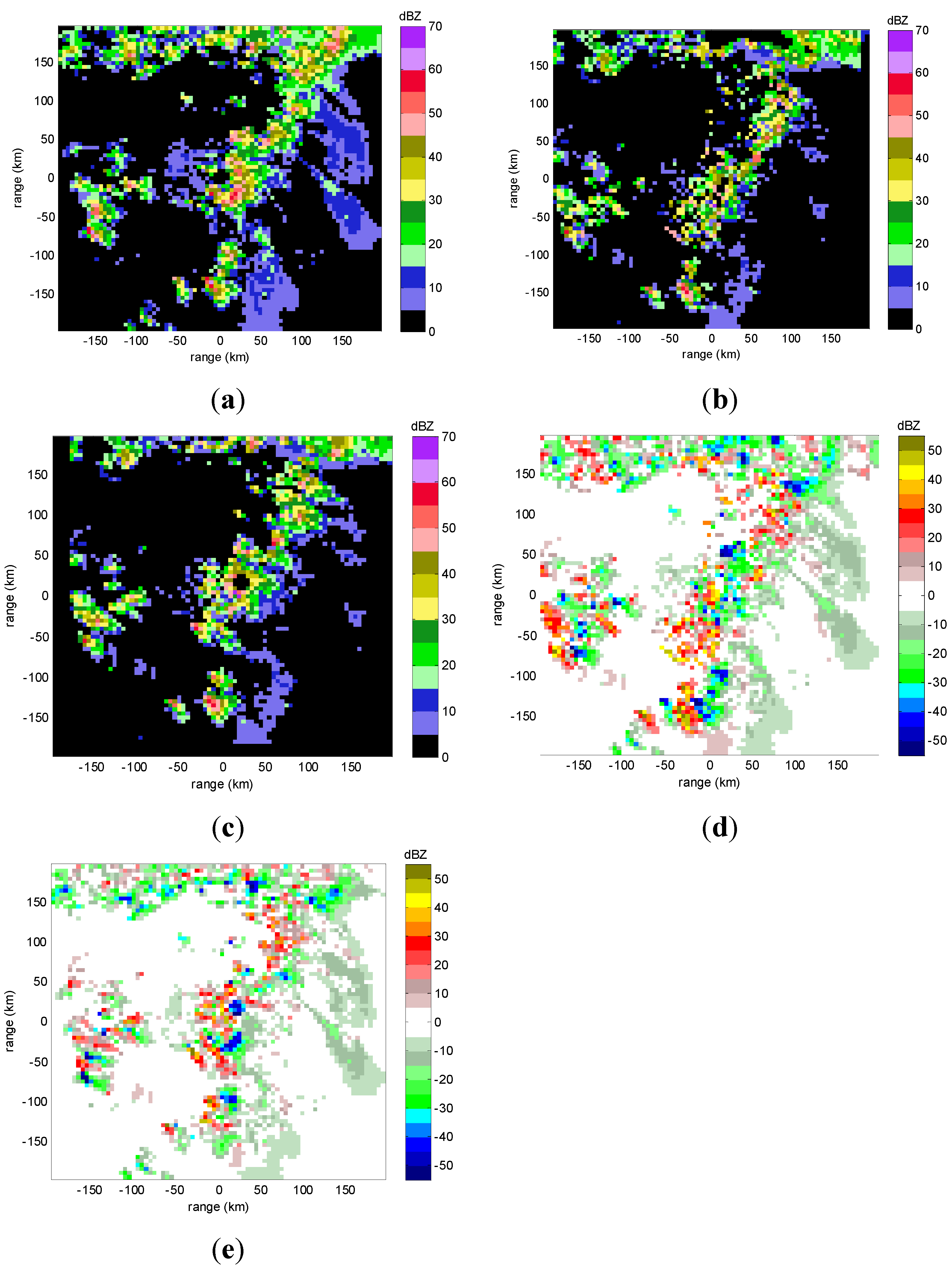
Figure 3 and Figure 4 show the radar reflectivity for the 30 min and 60 min forecast of the Changsha case. From the actual reflectivity and the forecasting reflectivity, as well as their difference, it can be seen that the reflectivity for the 30 min forecast is consistent with the actual reflectivity regarding the position and intensity, but the reflectivity for the 60 min forecast has obvious differences with the actual reflectivity. In addition, the cone of silence cannot move in reality but it may move in nowcasting using motion vectors provided by the methods. This false movement will cause incorrectness of calculation.

Figure 3. Radar reflectivity at 3 km height of the Changsha case at 12:56 (UTC) on 11 April 2006 with radar station at origin (0,0). (a) actual reflectivity; (b) forecasting reflectivity by COTREC; (c) forecasting reflectivity by GVAD; (d) difference between forecasting reflectivity by COTREC and actual reflectivity; (e) difference between forecasting reflectivity by GVAD and actual reflectivity.

Figure 3. Radar reflectivity at 3 km height of the Changsha case at 12:56 (UTC) on 11 April 2006 with radar station at origin (0,0). (a) actual reflectivity; (b) forecasting reflectivity by COTREC; (c) forecasting reflectivity by GVAD; (d) difference between forecasting reflectivity by COTREC and actual reflectivity; (e) difference between forecasting reflectivity by GVAD and actual reflectivity.

Figure 4. Radar reflectivity at 3 km height of the Changsha case at 13:26 (UTC) on 11 April 2006 with radar station at origin (0,0). (a) actual reflectivity; (b) forecasting reflectivity by COTREC; (c) forecasting reflectivity by GVAD; (d) difference between forecasting reflectivity by COTREC and actual reflectivity; (e) difference between forecasting reflectivity by GVAD and actual reflectivity.

Figure 4. Radar reflectivity at 3 km height of the Changsha case at 13:26 (UTC) on 11 April 2006 with radar station at origin (0,0). (a) actual reflectivity; (b) forecasting reflectivity by COTREC; (c) forecasting reflectivity by GVAD; (d) difference between forecasting reflectivity by COTREC and actual reflectivity; (e) difference between forecasting reflectivity by GVAD and actual reflectivity.

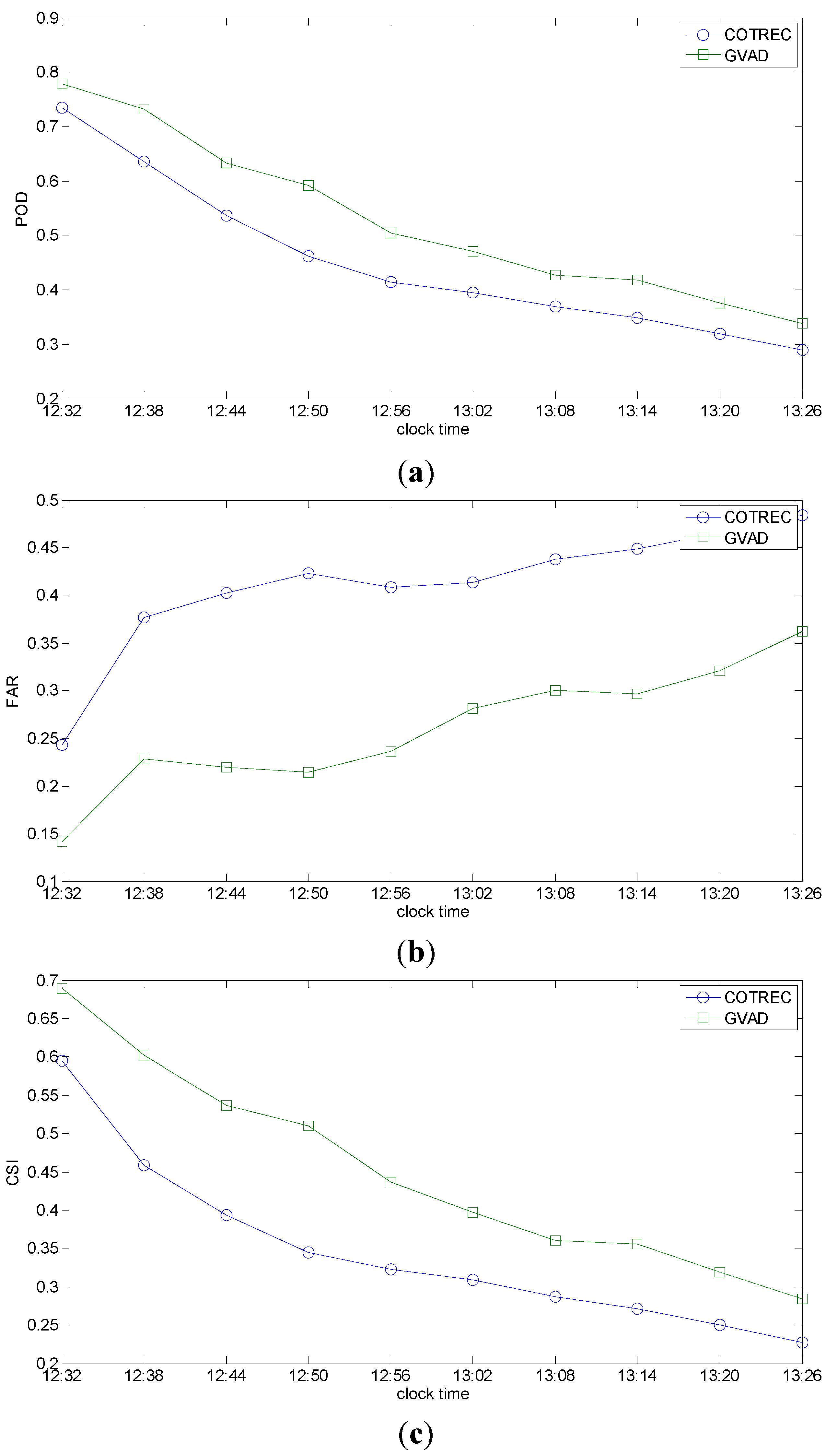
Figure 5 gives the testing results for each 6-min interval of the forecasting period from 12:32 to 13:26 (UTC). It can be seen that the POD of COTREC and GVAD both decrease, while FAR both increase as the forecasting time increases, and, thus, CSI of the two methods decrease evidently with the forecasting time. GVAD has a larger POD and a smaller FAR all the time, and, thus, has a larger CSI compared with COTREC. In this case, the performance of GVAD is obviously better than COTREC. As described in Table 2, this is a case of convective precipitation and it is apparently evolving during the 1-h forecasting time period. The main reason for the difference between the nowcasting results and the actual reflectivity is the rapid change of convective precipitation in the evolution. Since nowcasting is used to extrapolate the reflectivity in future with fixed motion vectors calculated at the initial time, the difference between the actual reflectivity and the reflectivity at the initial time increases with time due to the rapid evolution of the precipitation, which is unfavorable to determine the location and intensity of reflectivity in future. Because COTREC uses multiple motion vectors to implement extrapolation, based on the reflectivity at the initial time, while GVAD uses the environmental wind which is relative stable with time, COTREC is affected more than GVAD when the evolution of precipitation is significant, and, thus, the results of COTREC have a larger difference with the actual echoes.

Figure 5. Testing of the Changsha case for each 6-min interval from 12:32 to 13:26 (UTC) on 11 April 2006. (a) POD; (b) FAR; (c) CSI.

Figure 5. Testing of the Changsha case for each 6-min interval from 12:32 to 13:26 (UTC) on 11 April 2006. (a) POD; (b) FAR; (c) CSI.

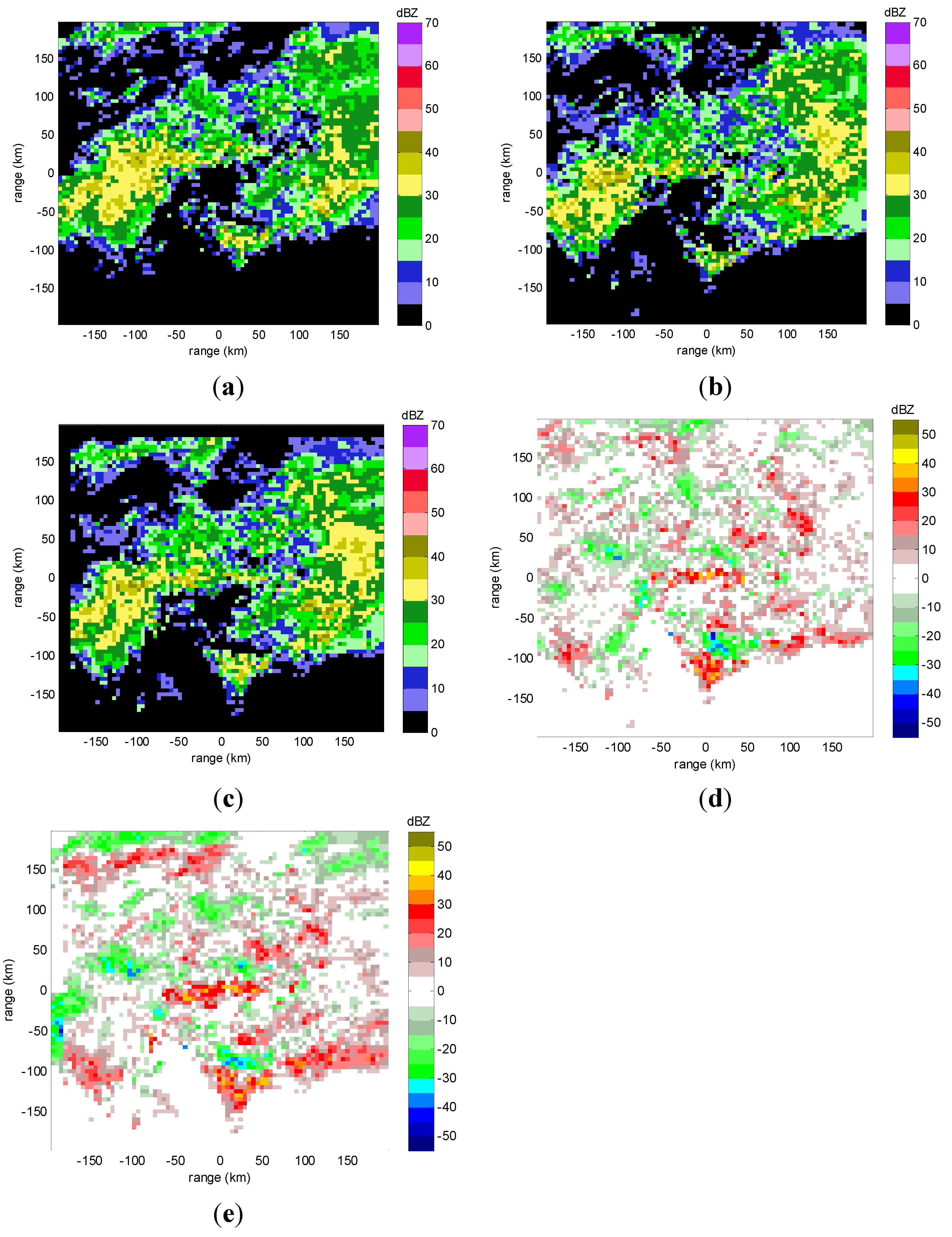
Figure 6 and Figure 7 show the radar reflectivity for the 30 min and 60 min forecasts of the Nanjing case. Compared with the convective case presented above, the forecasting results are more consistent with the actual reflectivity for this large scale precipitation.

Figure 6. Radar reflectivity at 3 km height of the Nanjing case at 00:30 (UTC) on 12 July 2010 with radar station at origin (0,0). (a) actual reflectivity; (b) forecasting reflectivity by COTREC; (c) forecasting reflectivity by GVAD; (d) difference between forecasting reflectivity by COTREC and actual reflectivity; (e) difference between forecasting reflectivity by GVAD and actual reflectivity.

Figure 6. Radar reflectivity at 3 km height of the Nanjing case at 00:30 (UTC) on 12 July 2010 with radar station at origin (0,0). (a) actual reflectivity; (b) forecasting reflectivity by COTREC; (c) forecasting reflectivity by GVAD; (d) difference between forecasting reflectivity by COTREC and actual reflectivity; (e) difference between forecasting reflectivity by GVAD and actual reflectivity.

Figure 7. Radar reflectivity at 3 km height of the Nanjing case at 01:00 (UTC) on 12 July 2010 with radar station at origin (0,0). (a) actual reflectivity; (b) forecasting reflectivity by COTREC; (c) forecasting reflectivity by GVAD; (d) difference between forecasting reflectivity by COTREC and actual reflectivity; (e) difference between forecasting reflectivity by GVAD and actual reflectivity.

Figure 7. Radar reflectivity at 3 km height of the Nanjing case at 01:00 (UTC) on 12 July 2010 with radar station at origin (0,0). (a) actual reflectivity; (b) forecasting reflectivity by COTREC; (c) forecasting reflectivity by GVAD; (d) difference between forecasting reflectivity by COTREC and actual reflectivity; (e) difference between forecasting reflectivity by GVAD and actual reflectivity.

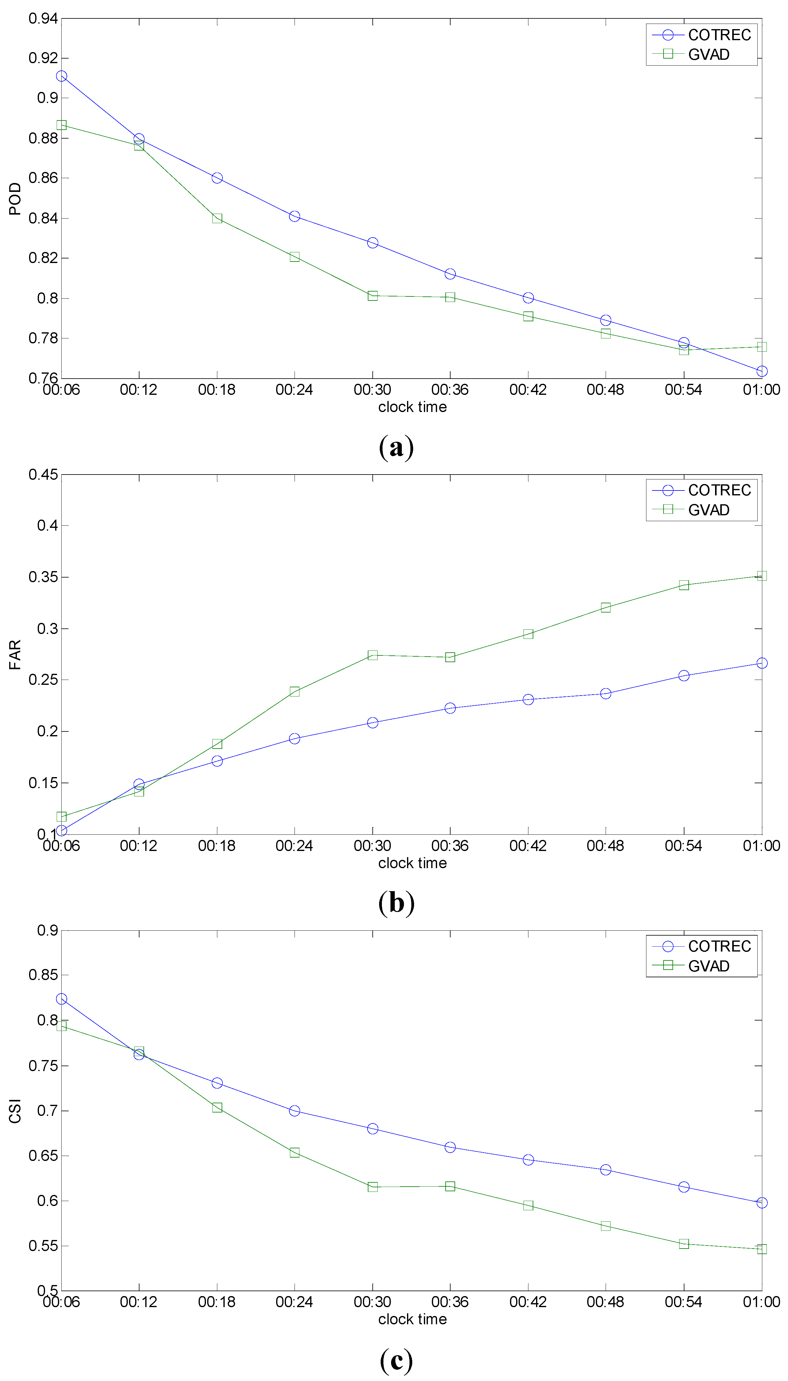
Figure 8 gives the testing results for each 6 min from 00:06 to 01:00 (UTC). It can be seen that the POD of the two methods have the same trends of decrease with the forecasting time. The FAR of the two methods have the same trends of increase with the forecasting time, but COTREC shows a smaller increase than GVAD. With regards to CSI during the forecasting period, COTREC gives better nowcasting than GVAD. As described in Table 2, this case is a stratiform precipitation and it is stable during the 1-h forecasting time period. The difference between actual reflectivity and the reflectivity at the initial time is small since the evolution of the precipitation is very slow. In this situation, compared with the uniform environmental wind calculated by GVAD, the multiple motion vectors calculated by COTREC can yield a more detailed and accurate trend within the 1-h forecasting time period and, thus, COTREC gives a better performance than GVAD.

Figure 8. Testing of the Nanjing case for each 6 min from 00:06 to 01:00 (UTC) on 12 July 2010. (a) POD; (b) FAR; (c) CSI.

Figure 8. Testing of the Nanjing case for each 6 min from 00:06 to 01:00 (UTC) on 12 July 2010. (a) POD; (b) FAR; (c) CSI.

The performance of the two methods for all the 11 cases can be referred to in Table 3, which gives the CSI scores for each 6 min interval in the 1-h nowcasting. Similar to the two presented cases, it can be seen in Table 3 that, for cases of evolving convective or mixed precipitation, such as Nanjing 19 April 2008, Nanjing 22 July 2008, Nanjing 1 July 2007, Wuhan 1 July 2007, Wuhan 3 May 2008, and Guangzhou 20 March 2013, GVAD gives better nowcasting than COTREC, while for cases of stable stratiform precipitation, such as Yantai 12 August 2010, COTREC gives better nowcasting than GVAD. For the other two convective or mixed cases with slow evolution and weak environmental wind, including Wuhan 10 July 2008 and Nanning 9 July 2011, COTREC and GVAD give similar nowcasting results. These two cases are neither stable stratiform precipitation nor convective or mixed precipitation with remarkable evolution, but lie between the two categories, therefore COTREC and GVAD show similar performance.

Table 3. CSI scores of the 11 cases for 10 extrapolation times of each 6 min in 1 hour nowcasting. Better performance between COTREC and GVAD is highlighted in bold type.

Case	Method	1	2	3	4	5	6	7	8	9	10
Nanjing 19 April 2008	COTREC	0.8189	0.7635	0.7421	0.7259	0.7059	0.6902	0.6738	0.6599	0.6354	0.6291
	GVAD	0.8347	0.8153	0.7620	0.7584	0.7467	0.7436	0.7107	0.7155	0.7049	0.7034
Nanjing 22 July 2008	COTREC	0.8490	0.7801	0.7288	0.6817	0.6438	0.5968	0.5556	0.5258	0.4998	0.4665
	GVAD	0.8523	0.7784	0.7266	0.7117	0.6769	0.6210	0.5905	0.5639	0.5353	0.5304
Nanjing 12 July 2010	COTREC	0.8242	0.7623	0.7305	0.6999	0.6795	0.6589	0.6452	0.6339	0.6150	0.5976
	GVAD	0.7935	0.7656	0.7030	0.6530	0.6150	0.6159	0.5948	0.5717	0.5520	0.5461
Nanjing 1 July 2007	COTREC	0.7031	0.6052	0.4758	0.4942	0.4693	0.4398	0.4011	0.3717	0.3534	0.3228
	GVAD	0.6632	0.6252	0.4870	0.4908	0.4670	0.4518	0.4246	0.3954	0.3884	0.3567
Wuhan 10 July 2008	COTREC	0.6559	0.5247	0.4498	0.4115	0.3733	0.3664	0.3460	0.3172	0.3045	0.2989
	GVAD	0.6879	0.5595	0.4827	0.4356	0.3872	0.3704	0.3457	0.3266	0.3092	0.3009
Wuhan 1 July 2008	COTREC	0.8236	0.7459	0.6811	0.6447	0.6100	0.5913	0.5680	0.5480	0.5262	0.4940
	GVAD	0.8471	0.7686	0.7522	0.6964	0.6815	0.6447	0.6475	0.6103	0.6077	0.5664
Wuhan 3 May 2008	COTREC	0.8130	0.7597	0.7113	0.6977	0.6555	0.6343	0.6079	0.5885	0.5678	0.5553
	GVAD	0.8122	0.7591	0.7215	0.7004	0.6764	0.6462	0.6353	0.6334	0.6220	0.6200
Changsha 11 April 2006	COTREC	0.5944	0.4591	0.3938	0.3451	0.3224	0.3085	0.2866	0.2714	0.2498	0.2273
	GVAD	0.6895	0.6021	0.5371	0.5099	0.4364	0.3974	0.3606	0.3555	0.3189	0.2841
Nanning 9 July 2011	COTREC	0.6051	0.5222	0.4577	0.3985	0.3775	0.3638	0.3356	0.3059	0.2866	0.2738
	GVAD	0.6051	0.5307	0.4892	0.3821	0.3795	0.3702	0.3224	0.3326	0.2638	0.2505
Guangzhou 20 March 2013	COTREC	0.6037	0.4110	0.2933	0.2255	0.1865	0.1693	0.1548	0.1636	0.1703	0.1613
	GVAD	0.5668	0.4369	0.3471	0.3306	0.3050	0.2809	0.2828	0.2660	0.2428	0.2456
Yantai 12 August 2010	COTREC	0.8404	0.7821	0.7423	0.7076	0.6786	0.6532	0.6201	0.5933	0.5812	0.5539
	GVAD	0.8478	0.7911	0.7442	0.6973	0.6038	0.5744	0.5481	0.5164	0.4913	0.4517

Table 3. CSI scores of the 11 cases for 10 extrapolation times of each 6 min in 1 hour nowcasting. Better performance between COTREC and GVAD is highlighted in bold type.

Case	Method	1	2	3	4	5	6	7	8	9	10
Nanjing 19 April 2008	COTREC	0.8189	0.7635	0.7421	0.7259	0.7059	0.6902	0.6738	0.6599	0.6354	0.6291
	GVAD	0.8347	0.8153	0.7620	0.7584	0.7467	0.7436	0.7107	0.7155	0.7049	0.7034
Nanjing 22 July 2008	COTREC	0.8490	0.7801	0.7288	0.6817	0.6438	0.5968	0.5556	0.5258	0.4998	0.4665
	GVAD	0.8523	0.7784	0.7266	0.7117	0.6769	0.6210	0.5905	0.5639	0.5353	0.5304
Nanjing 12 July 2010	COTREC	0.8242	0.7623	0.7305	0.6999	0.6795	0.6589	0.6452	0.6339	0.6150	0.5976
	GVAD	0.7935	0.7656	0.7030	0.6530	0.6150	0.6159	0.5948	0.5717	0.5520	0.5461
Nanjing 1 July 2007	COTREC	0.7031	0.6052	0.4758	0.4942	0.4693	0.4398	0.4011	0.3717	0.3534	0.3228
	GVAD	0.6632	0.6252	0.4870	0.4908	0.4670	0.4518	0.4246	0.3954	0.3884	0.3567
Wuhan 10 July 2008	COTREC	0.6559	0.5247	0.4498	0.4115	0.3733	0.3664	0.3460	0.3172	0.3045	0.2989
	GVAD	0.6879	0.5595	0.4827	0.4356	0.3872	0.3704	0.3457	0.3266	0.3092	0.3009
Wuhan 1 July 2008	COTREC	0.8236	0.7459	0.6811	0.6447	0.6100	0.5913	0.5680	0.5480	0.5262	0.4940
	GVAD	0.8471	0.7686	0.7522	0.6964	0.6815	0.6447	0.6475	0.6103	0.6077	0.5664
Wuhan 3 May 2008	COTREC	0.8130	0.7597	0.7113	0.6977	0.6555	0.6343	0.6079	0.5885	0.5678	0.5553
	GVAD	0.8122	0.7591	0.7215	0.7004	0.6764	0.6462	0.6353	0.6334	0.6220	0.6200
Changsha 11 April 2006	COTREC	0.5944	0.4591	0.3938	0.3451	0.3224	0.3085	0.2866	0.2714	0.2498	0.2273
	GVAD	0.6895	0.6021	0.5371	0.5099	0.4364	0.3974	0.3606	0.3555	0.3189	0.2841
Nanning 9 July 2011	COTREC	0.6051	0.5222	0.4577	0.3985	0.3775	0.3638	0.3356	0.3059	0.2866	0.2738
	GVAD	0.6051	0.5307	0.4892	0.3821	0.3795	0.3702	0.3224	0.3326	0.2638	0.2505
Guangzhou 20 March 2013	COTREC	0.6037	0.4110	0.2933	0.2255	0.1865	0.1693	0.1548	0.1636	0.1703	0.1613
	GVAD	0.5668	0.4369	0.3471	0.3306	0.3050	0.2809	0.2828	0.2660	0.2428	0.2456
Yantai 12 August 2010	COTREC	0.8404	0.7821	0.7423	0.7076	0.6786	0.6532	0.6201	0.5933	0.5812	0.5539
	GVAD	0.8478	0.7911	0.7442	0.6973	0.6038	0.5744	0.5481	0.5164	0.4913	0.4517

t test is implemented to statistically see the performance differences for the 11 cases using CSI scores in Table 3. Given significance level of 99%, COTREC is better than GVAD for Nanjing 1 July 2007, Wuhan 10 July 2008, Nanning 9 July 2011 and Yantai 12 August 2010, and GVAD is better than COTREC for Nanjing 19 April 2008, Nanjing 22 July 2008, Nanjing 1 July 2007, Wuhan 10 July 2008, Wuhan 1 July 2008, Wuhan 3 May 2008, Changsha 11 April 2006, Nanning 9 July 2011, and Guangzhou 20 March 2013. The statistical test give similar results as those discussed above and justify that GVAD can be used in nowcasting.

5. Conclusions

In this study, multiple wind retrieval algorithms are applied in nowcasting, based on the reflectivity data or radial velocity data of Doppler weather radars. The COTREC and GVAD methods are used to obtain horizontal wind fields, at a height of 3 km, which are treated as motion vectors of radar reflectivity at the same height to give reflectivity forecast within 60 min. Based on the nowcasting results of 11 typical precipitation events by the two methods, the following conclusions can be drawn:

(1)

Wind retrieval algorithms, using radial velocity data provided by Doppler weather radars, such as GVAD, can give reasonable nowcasting results compared with commonly used nowcasting methods using reflectivity data, such as COTREC. Therefore, GVAD can be used in nowcasting as COTREC performs.

(2)

For stable stratiform precipitation, the performance of COTREC is better than GVAD in nowcasting, while for evolving convective or mixed precipitation, the performance of GVAD is better than COTREC. According to this, a suitable method can be chosen in operational nowcasting.

The nowcasting results may be related to the growth and decay of echoes and the change of wind fields, for which current extrapolation nowcasting methods do not take into account. Further analysis with more samples is needed to discuss these issues. An improved algorithm is also under study to give more accurate results.