1. Introduction
For climate change impact assessment, as well as for the design and evaluation of climate change adaptation measures, spatially high-resolution information on potential future regional climate changes is needed (e.g., [
1,
2]). This information can be provided by regional climate models (RCMs), which are used to refine the climate change information provided by global climate models (GCMs) on a much coarser spatial resolution. The GCMs are fed by potential future evolutions of concentrations of greenhouse gases and aerosols (or emissions in the case of recent Earth system models). One combination of emission scenario, GCM and RCM, results in one single possible future climate evolution for a region. Using a different GCM, a different RCM or assuming a different emission scenario gives a second possible future, and so on. However, it is not possible to decide which one is more likely.
There are three main sources contributing to this uncertainty. The first one is the unknown development of future anthropogenic greenhouse gas emissions and the partly unknown future storage capacities of the biosphere and the oceans. A second contribution to the uncertainty is the models themselves, which do not represent all processes of the climate system perfectly and which might represent different processes unequally well. Thirdly, the non-linearity of the processes constituting the climate system creates non-deterministic variability and prevents a clear identification of changing climate conditions from the climate simulations. These sources of uncertainty of climate projections have been described and analyzed in detail (e.g., [
3,
4]).
Some aspects of the uncertainty of climate projections have the potential to be reduced. A very important approach to address the uncertainty of climate projections is the improvement of process understanding and, thereby, the reduction of model biases [
3]. In addition, increasing the spatial and temporal resolution of the simulations can lead to better representation of today’s climate by the models, including a more realistic representation of the variability and extreme event statistics [
5,
6]. This model improvement is the basis for the applied usage of climate simulation data. However, it cannot reduce the uncertainties related to the unknown future greenhouse gas emissions and to the natural internal variability of the climate system. It was shown that large parts of the uncertainty range (defined by two standard deviations) of the CMIP5 [
7] projections can be covered by the uncertainty range of an initial condition ensemble of one single model [
8]. This is especially true for the upcoming decades [
3,
9]. Decisions on adaptation to climate change are thus to be taken based on information provided by multi-model, multi-scenario and multi-realization ensembles of climate change simulations. For some climatic parameters, this information is (relatively) stringent, where the ensemble of simulations is showing a clear trend despite the possible bandwidth in the magnitude of the trend. For other climatic parameters, the ensemble results in less clear information, with disagreement not only in the magnitude, but also in the direction of the projected changes.
To assess the results of ensembles of climate change projections and to display not only mean projected climate changes, but also information on the robustness of the results, various approaches of ensemble compositions, model output statistics and visualization methods have been developed. In the context of the European FP7 project IMPACT2C, robust changes in mean and extreme temperature, precipitation, winds and surface energy budgets were identified for Europe under 2 °C global warming, using a simple metric of model agreement on the sign of the changes as indicator of robustness [
10]. A complex measure of robustness using cumulative density functions of the individual and multi-model mean projections to distinguish the signal from noise was applied to the global CMIP5 simulations. The authors concluded that the local spread of the simulations did not change substantially between CMIP3 and CMIP5 simulations [
11]. To overcome the large uncertainties in the projections of local extremes, a method of spatial aggregation was applied to an initial condition ensemble of one Earth system model. Despite large uncertainties on the local and short-term scale, this method shows that projections of extremes are remarkably consistent from an aggregated spatial probability perspective [
8]. The summary for policymakers of the 5th Assessment Report of the Intergovernmental Panel on Climate Change presents mean projected climate changes from an ensemble of global climate change simulations. The results are presented in a figure, including stippling of regions where model agreement is large and where the natural internal variability is small compared to the the multi-model mean change and hatching of regions where the natural internal variability is large compared to the multi-model mean change (Figure SPM-08a,b [
12,
13]). These figures comprise plenty of information, and this complexity makes it difficult to gather all information at once.
The aim of the present study is to reduce the complexity of such figures, in order to make them understandable, not only for climate experts, but also for decision makers from public administrations and from the economy. Here, we present the method of climate signal maps to derive and display the robustness of climate changes projected by an ensemble of regional climate change simulations. The method has similarities to the IPCC method described above, but gives simplified information understandable at a glance. The paper is structured as follows: After introducing the data basis and describing the method to test for robustness and to visualize the results (
Section 2 and
Section 3), an application of the method to projected changes of seasonal and extreme precipitation for Germany is presented in
Section 4. The results for two ensembles based on the representative concentration pathways (RCPs) 4.5 and 8.5 [
14] are compared to the results for an ensemble of simulations based on the emission scenario A1B as defined in the Special Report on Emission Scenarios (SRES [
15]). Concluding remarks are given in
Section 6.
4. Results
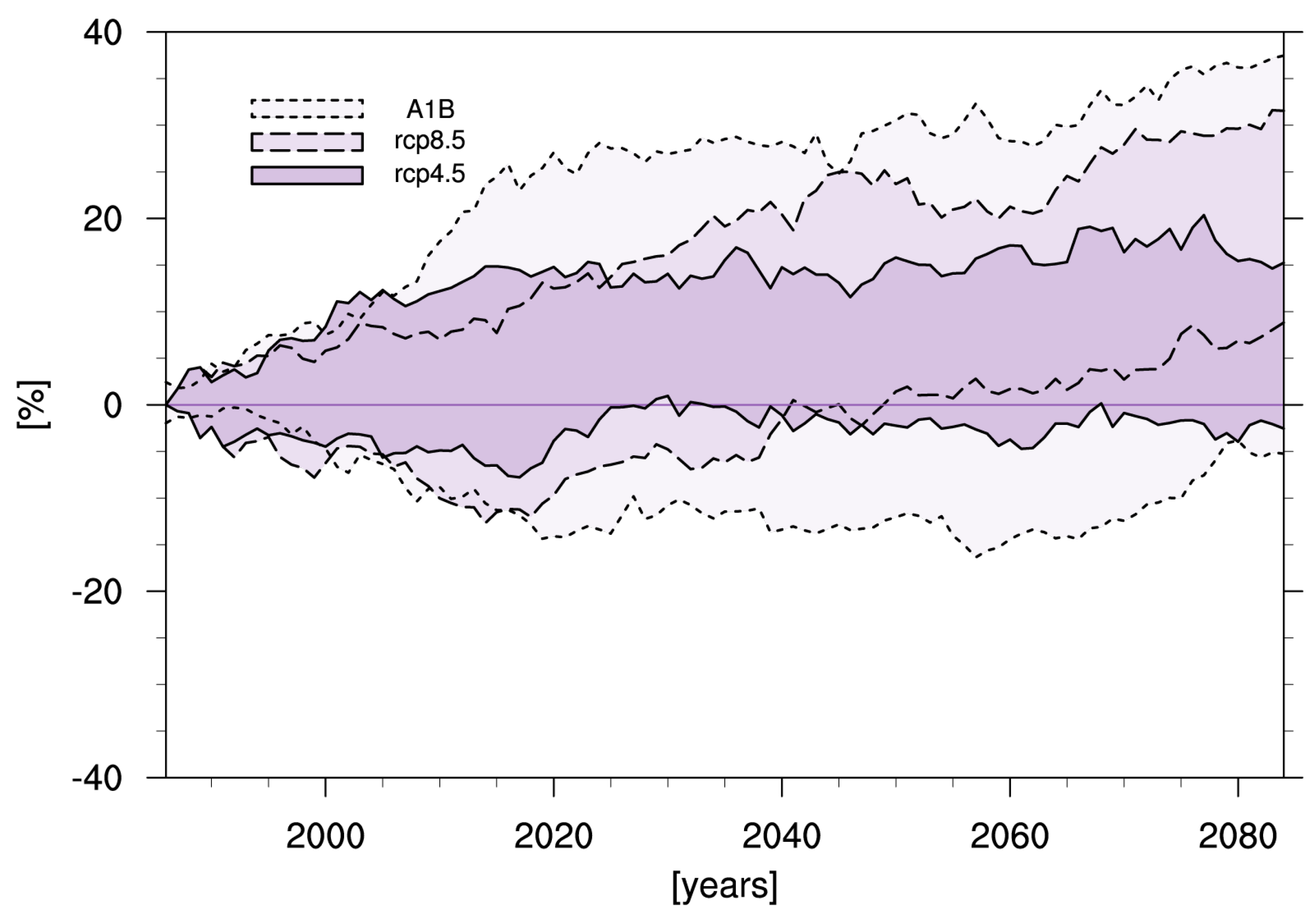
To illustrate the method of the climate signal maps, we show two types of figures. Firstly, time series of the projected changes are shown, which are based on 30-year running mean anomalies with respect to the reference period of 1971–2000 for each ensemble member. The data have been spatially averaged for the area of Germany. The figures show the envelope of the projections of the entire ensemble,
i.e., the lines denote the highest and the lowest changes. Note that values for different time steps may come from different models. The shaded areas represent the bandwidth given by the ensemble of simulations. Secondly, climate signal maps are shown for four different 30-year periods (2031–2060, 2041–2070, 2051–2080, 2061–2090), again with respect to the reference period of 1971–2000. Ensemble median changes are shown in the top panels, with low changes colored in green, medium changes in orange and larger changes in red. Ensemble median changes are used, because they are less influenced by single outliers than ensemble mean changes. For the lower panels, the robustness tests as described in
Section 3.2 were applied. Regions that failed in at least one of the tests are shown in gray.
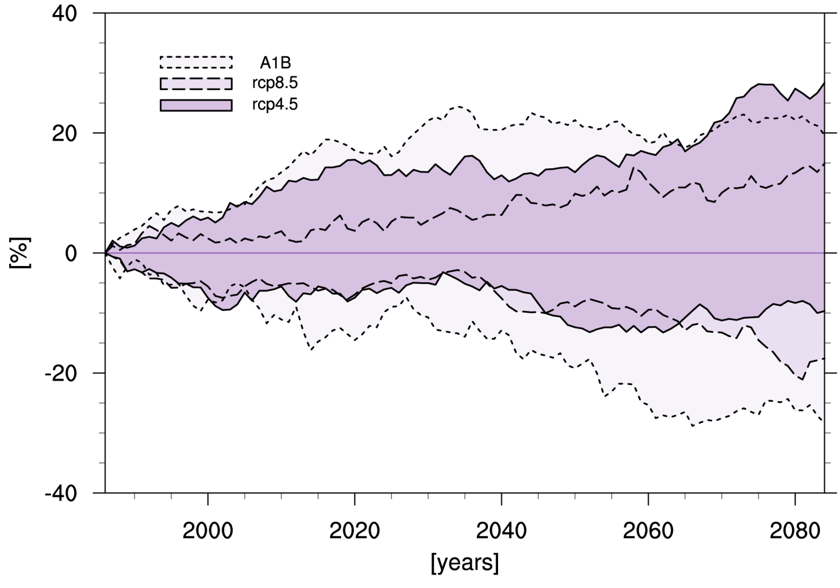
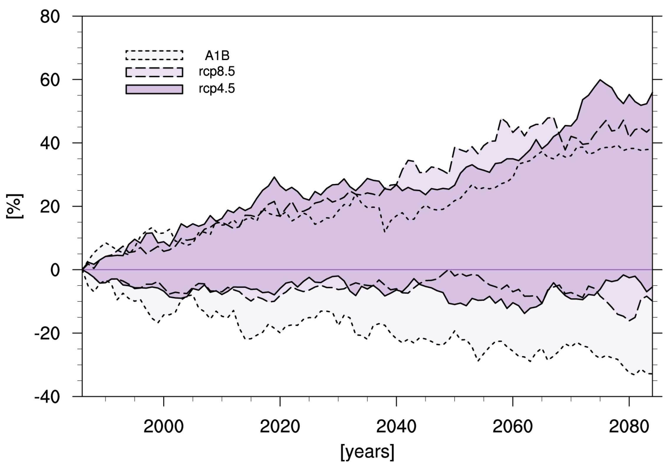
The projected changes in winter precipitation for the EURO-CORDEX RCP4.5 and RCP8.5 simulations and for the ENSEMBLES A1B simulations are shown in
Figure 1. The EURO-CORDEX simulations mostly project increasing winter precipitation, which gets more pronounced for the simulations based on RCP8.5 after 2040. However, the bandwidth of changes of the RCP4.5 simulations includes the zero-changes line for the entire period; for the RCP8.5 simulations, this is the case until about 2040. The bandwidth spanned by the ENSEMBLES simulations is much broader, already for the early decades from 2020.
Figure 1.
Projected change in winter precipitation (%). The figure shows the envelope of 30-year running mean anomalies with respect to the reference period of 1971–2000 for the ENSEMBLES A1B simulations (light gray area and dotted lines), for the EURO-CORDEX RCP8.5 simulations (medium gray area and dashed lines) and for the EURO-CORDEX RCP4.5 simulations (dark gray area and solid lines). The temporal means are mapped on the central year of the respective 30-year period.
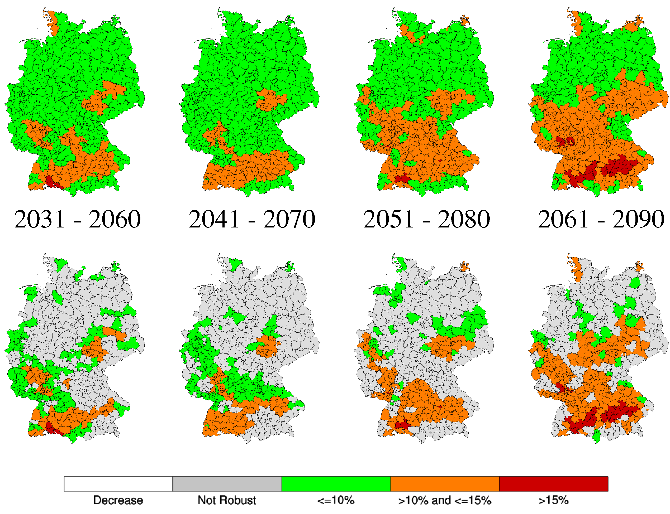
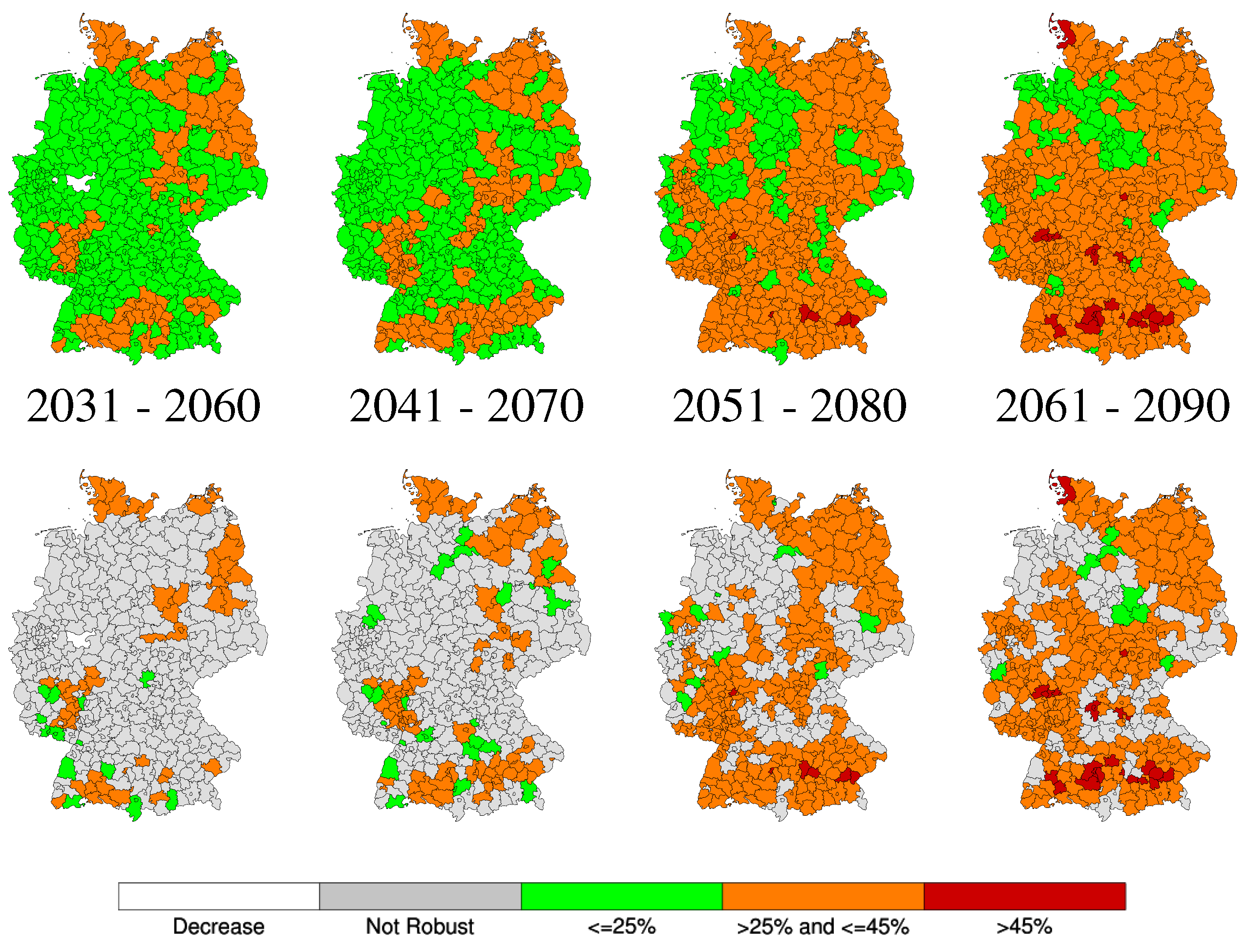
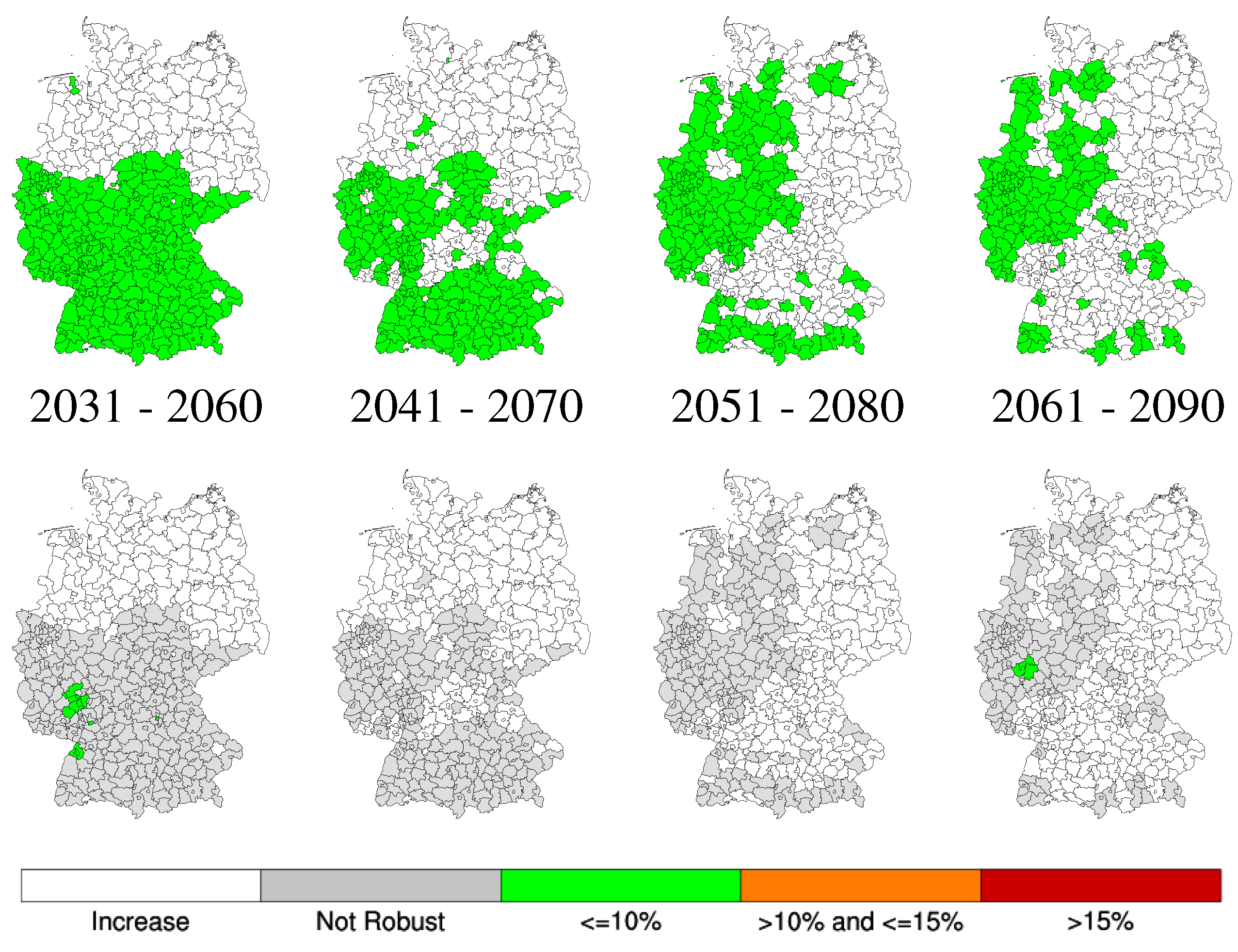
For the same data, climate signal maps are shown for the RCP4.5 (
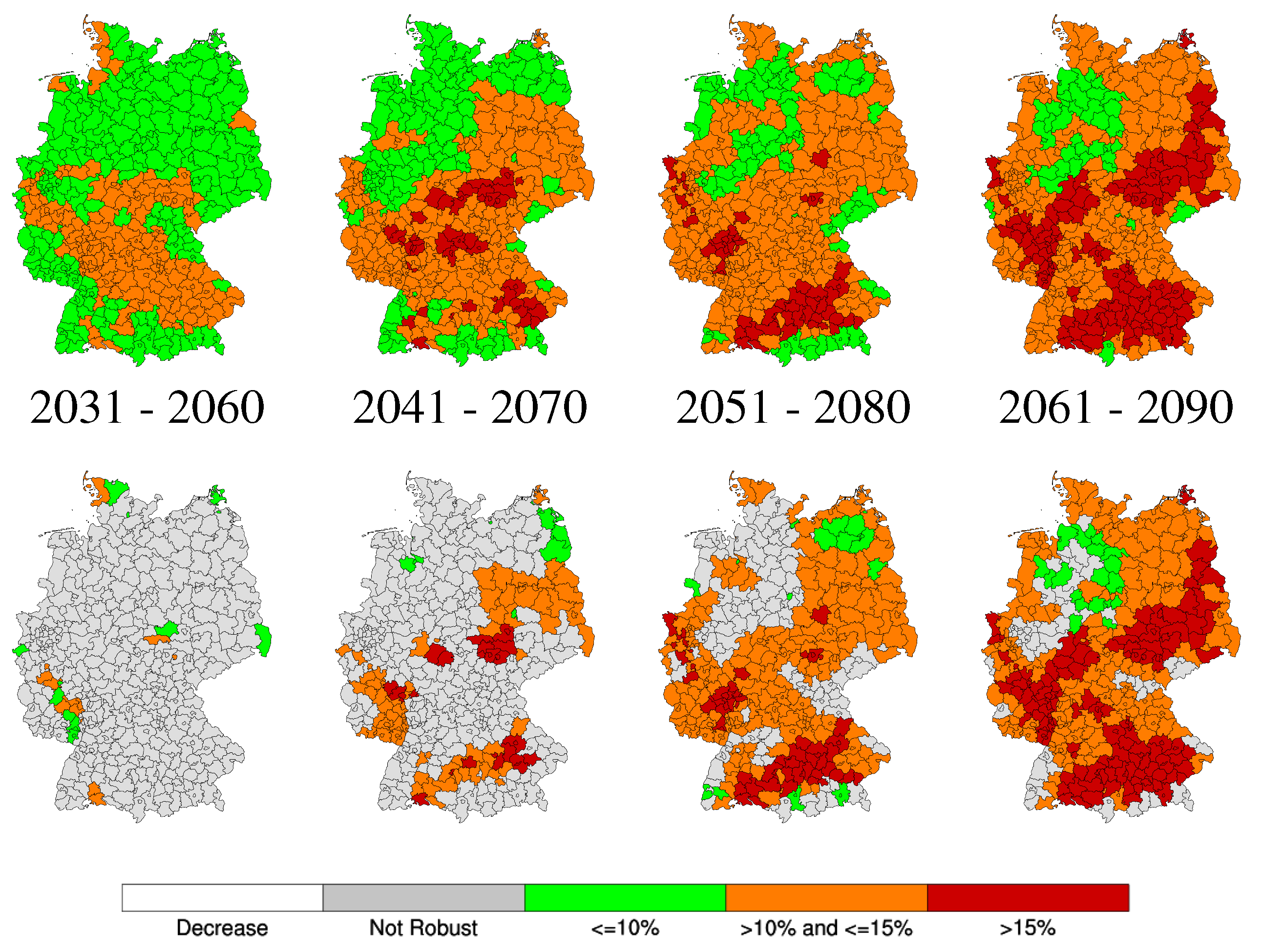
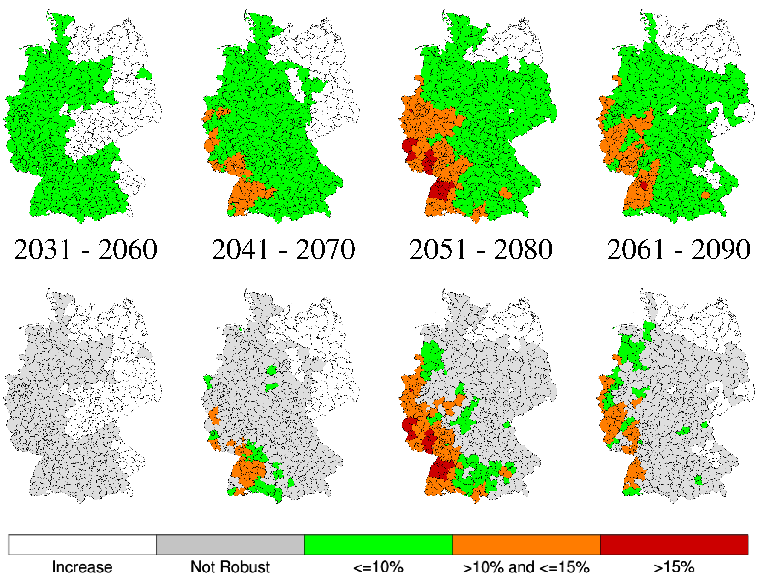
Figure 2), RCP8.5 (
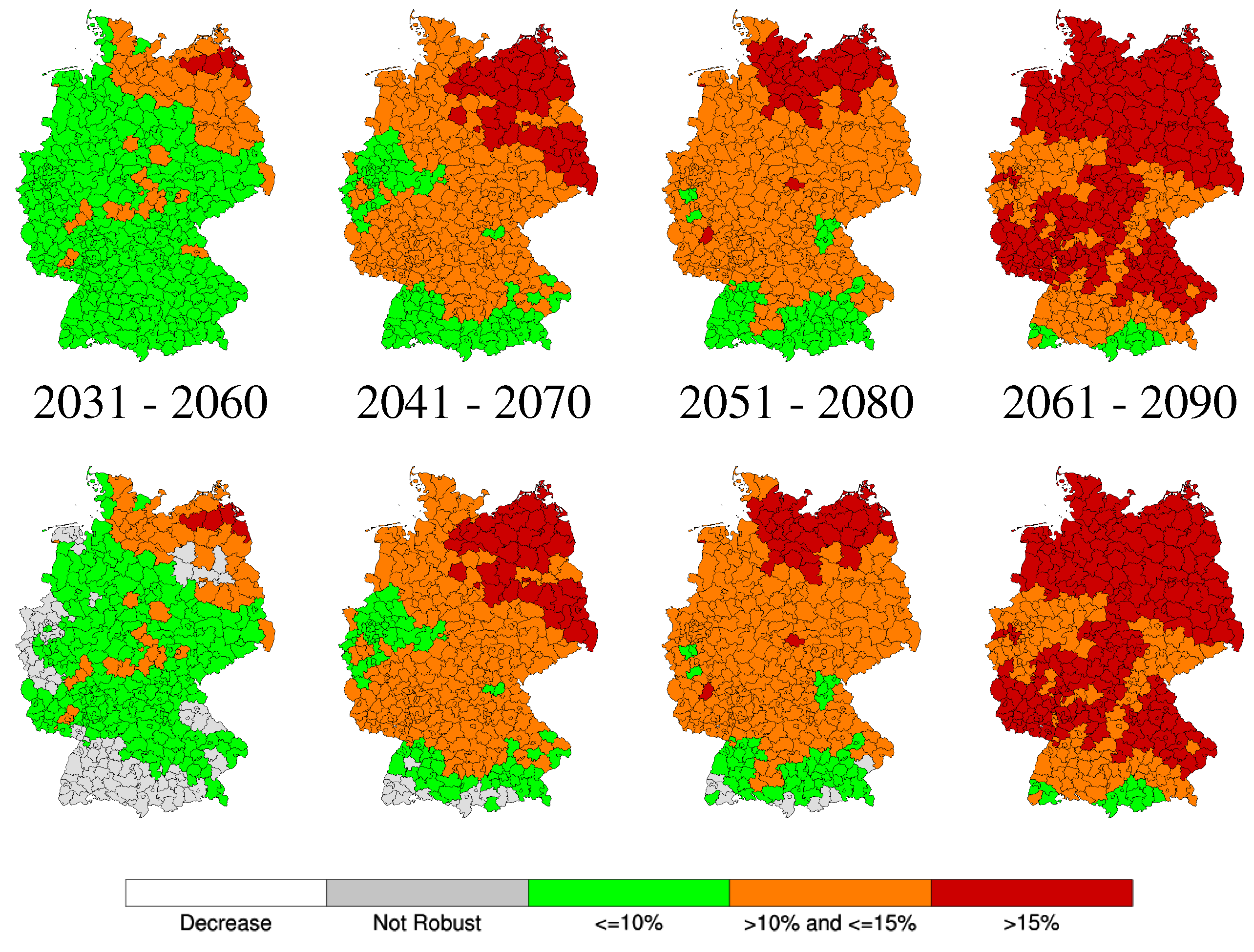
Figure 3) and A1B (
Figure 4) simulations. Interestingly, for the RCP4.5-based simulations, there are regions in southwestern Germany where the projected changes in winter precipitation are robust already for the near future time periods (2031–2060, 2041–2070) and stay robust until the end of the 21st century. For the RCP8.5-based simulations, regions with robust changes do not emerge prior to the 2041–2070 period, but cover larger parts of the country and show stronger changes.
Figure 2.
Increase of winter precipitation (%) for (from left to right) 2031–2060, 2041–2070, 2051–2080 and 2061–2090 compared to the reference period 1971–2000. Color coded: median of 10 RCM simulations from the EURO-CORDEX RCP4.5 simulations. For the top panels, no test was applied to the data. In the lower panels, regions that failed at least one of the two robustness tests are grayed out.
Figure 3.
Increase of winter precipitation (%) for (from left to right) 2031–2060, 2041–2070, 2051–2080 and 2061–2090 compared to the reference period 1971–2000. Color coded: median of 11 RCM simulations from the EURO-CORDEX RCP8.5 simulations. For the top panels, no test was applied to the data. In the lower panels, regions that failed at least one of the two robustness tests are grayed out.
Figure 4.
Increase of winter precipitation (%) for (from left to right) 2031–2060, 2041–2070, 2051–2080 and 2061–2090 compared to the reference period 1971–2000. Color coded: median of 15 RCM simulations from the ENSEMBLES A1B simulations. For the top panels, no test was applied to the data. In the lower panels, regions that failed at least one of the two robustness tests are grayed out.
The ENSEMBLES A1B simulations (
Figure 4) differ substantially from the EURO-CORDEX simulations (
Figure 2 and
Figure 3). Firstly, the regional patterns of winter precipitation increase differ. For the EURO-CORDEX simulations, the largest increase is projected for southern Germany for both the RCP4.5 and RCP8.5 ensemble. From the ENSEMBLES simulations, the strongest increase emerges for northeast Germany. This effect can be related to differences in the simulated changes in large-scale circulation patterns between the CMIP3 models [
28], which are the basis for the regional ENSEMBLES simulations and the CMIP5 models, building the basis for the EURO-CORDEX simulations [
29]. Secondly, the ENSEMBLES A1B projections for increasing winter precipitation are identified as robust already for the early time periods for most of Germany. This is unexpected considering the large bandwidth of the projections (
Figure 1). However, the bandwidth might be misleading in this case, as the negative changes are projected by two simulations only (both driven by the same GCM). The test for agreement was passed, as two simulations out of an ensemble of 15 simulations are less than the requested 34% deviant changes, which would cause a test failure.
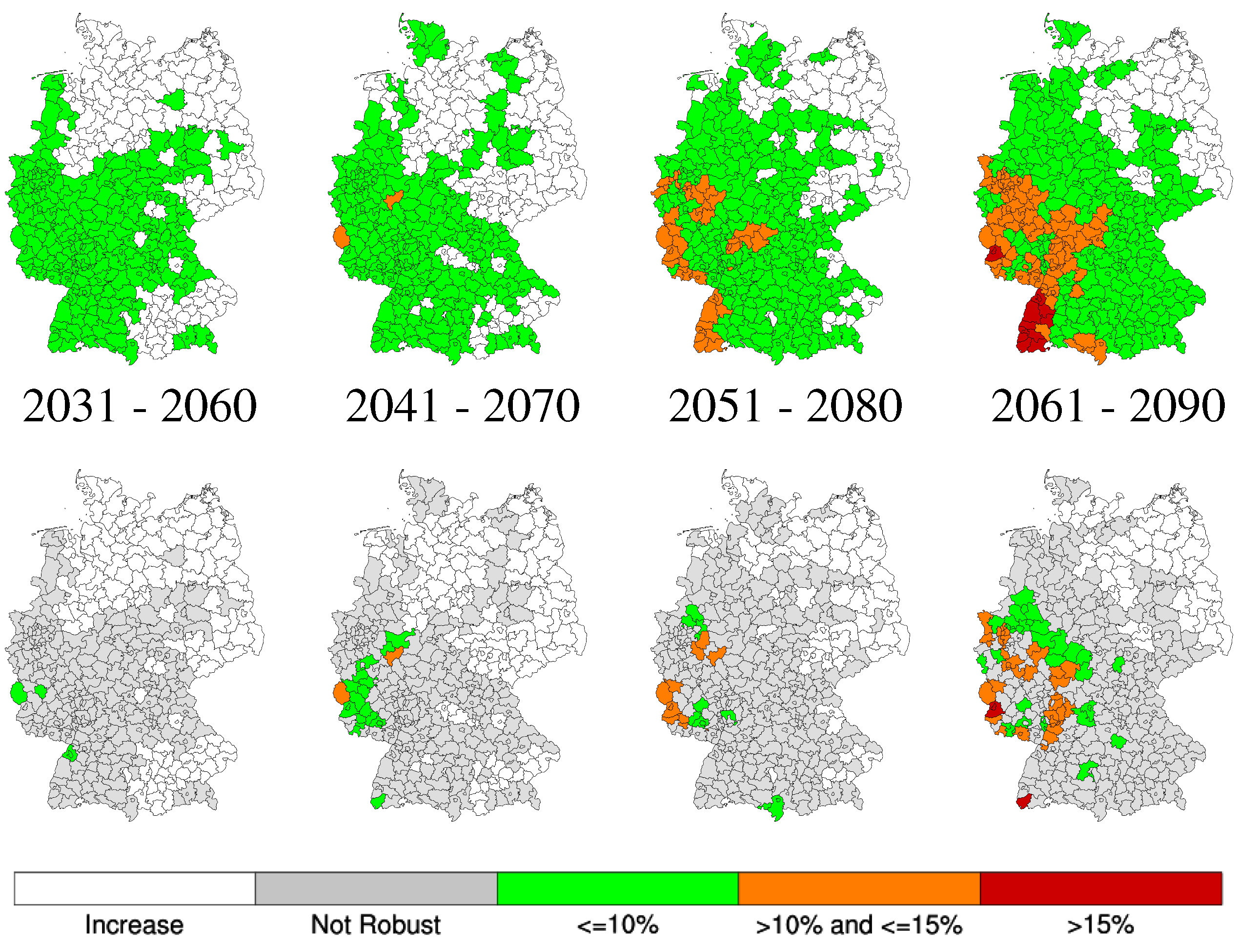
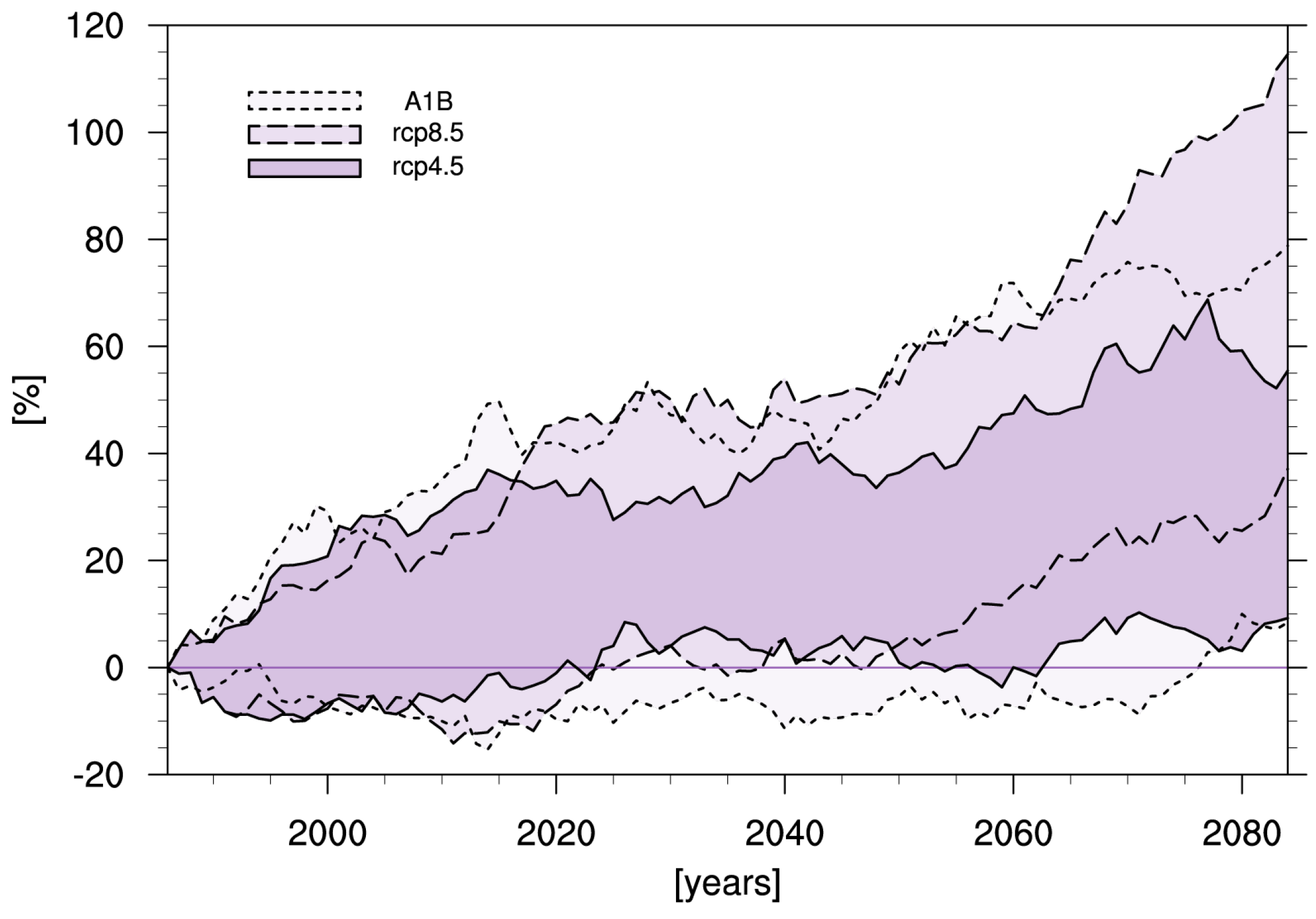
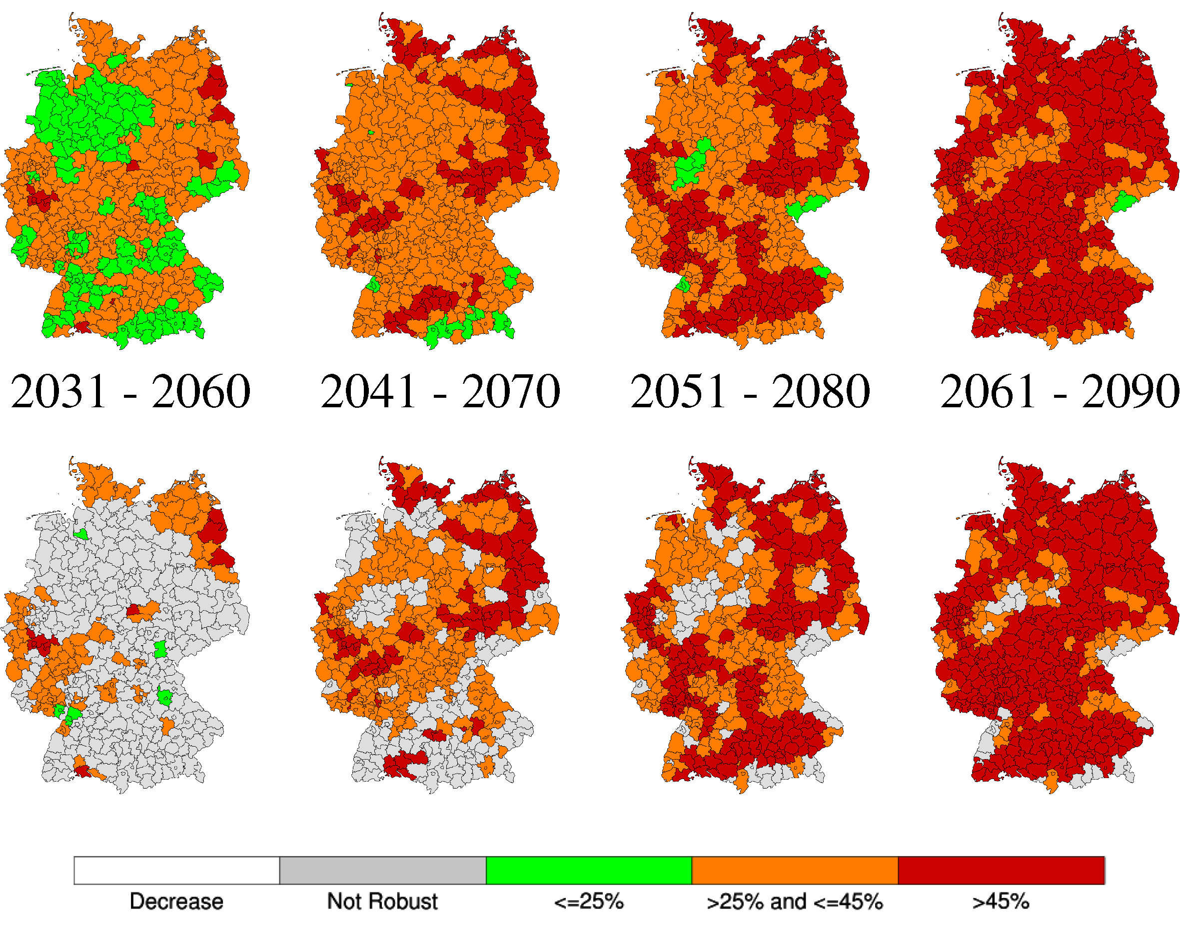
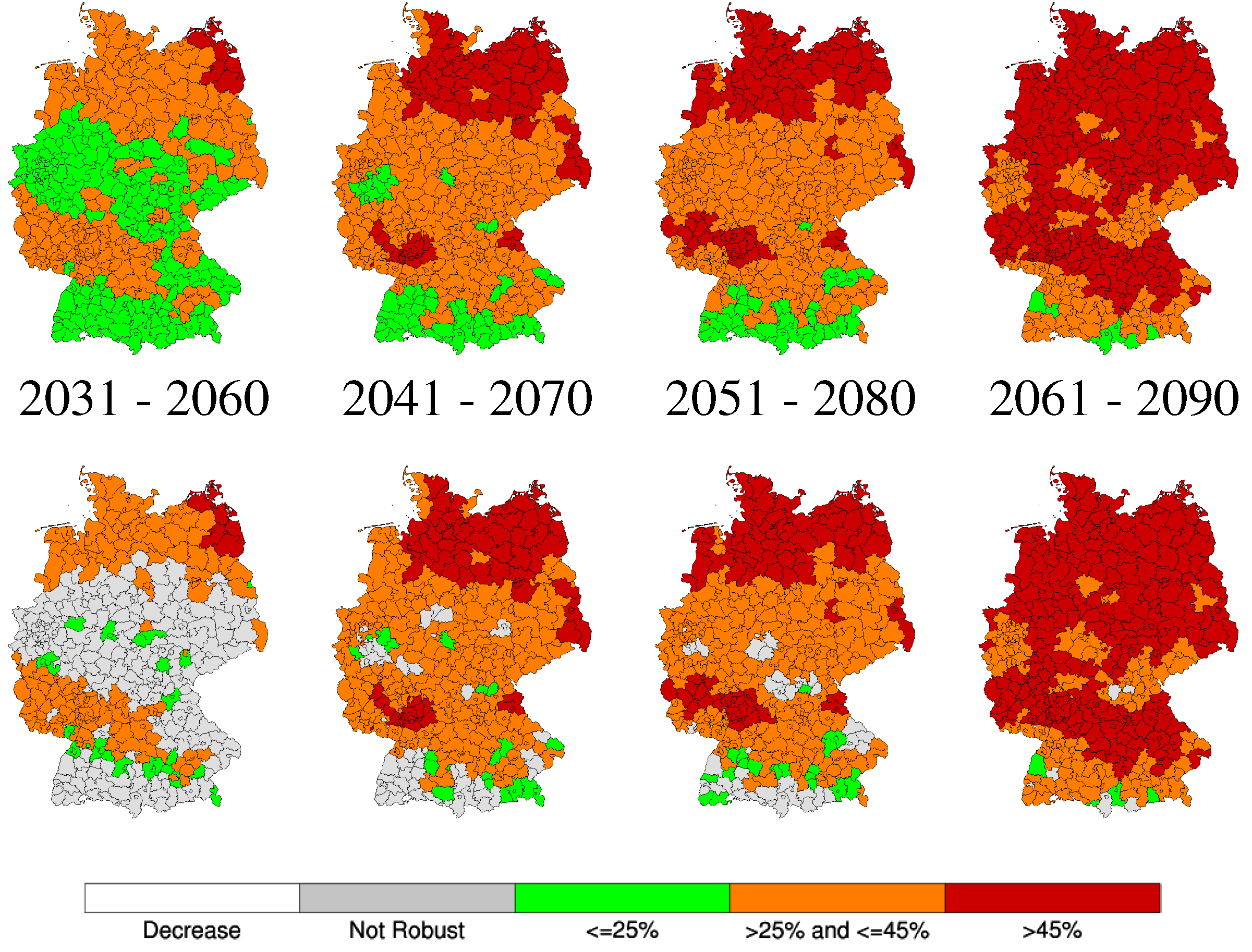
The projected changes in summer precipitation are shown in
Figure 5,
Figure 6,
Figure 7 and
Figure 8. From the time series (
Figure 5), no clear trend of domain-averaged summer precipitation change (neither an increase, nor decrease) can be derived. Instead, all three ensembles enclose the zero-changes line in their bandwidth, with highest increases projected by the ensemble of RCP4.5 simulations towards the end of the 21st century. As for winter precipitation, the ENSEMBLES ensemble again gives a broader bandwidth with stronger decreases towards the end of the 21st century.
Figure 5.
Projected change in summer precipitation (%). The figure shows the envelope of 30-year running mean anomalies with respect to the reference period of 1971–2000 for the ENSEMBLES A1B simulations (light gray area and dotted lines), for the EURO-CORDEX RCP8.5 simulations (medium gray area and dashed lines) and for the EURO-CORDEX RCP4.5 simulations (dark gray area and solid lines). The temporal means are mapped on the central year of the respective 30-year period.
Figure 6.
Decrease of summer precipitation (%) for (from left to right) 2031–2060, 2041–2070, 2051–2080 and 2061–2090 compared to the reference period 1971–2000. Color coded: median of 10 RCM simulations from the EURO-CORDEX RCP4.5 simulations. For the top panels, no test was applied to the data. In the lower panels, regions that failed at least one of the two robustness tests are grayed out.
Figure 7.
Decrease of summer precipitation (%) for (from left to right) 2031–2060, 2041–2070, 2051–2080 and 2061–2090 compared to the reference period 1971–2000. Color coded: median of 11 RCM simulations from the EURO-CORDEX RCP8.5 simulations. For the top panels, no test was applied to the data. In the lower panels, regions that failed at least one of the two robustness tests are grayed out.
Figure 8.
Decrease of summer precipitation (%) for (from left to right) 2031–2060, 2041–2070, 2051–2080 and 2061–2090 compared to the reference period 1971–2000. Color coded: median of 15 RCM simulations from the ENSEMBLES A1B simulations. For the top panels, no test was applied to the data. In the lower panels, regions that failed at least one of the two robustness tests are grayed out.
Here, the climate signal map method is used to check for the existence of regions where a robust decrease of the summer precipitation can be derived from the data. This is shown in
Figure 6,
Figure 7 and
Figure 8. For RCP4.5 (
Figure 6), the median decrease of summer precipitation is weak and basically limited to southern Germany until about 2075 and to western Germany thereafter. As could be expected from
Figure 5, the climate signal map method does not indicate any robust decrease in the projected summer precipitation for the RCP4.5 simulations.
For RCP8.5, however, the climate signal maps indicate regions with robust projections of decreasing summer precipitation.
Figure 7 shows temporally expanding and intensifying regions in southwestern Germany where summer precipitation is projected to decrease and which start to become robust towards the end of the 21st century. The ENSEMBLES ensemble projects decreases in summer precipitation that are relatively similar to those projected by the EURO-CORDEX RCP8.5 ensemble in terms of location and intensity of the strongest changes.
The comparatively low radiative forcing of RCP4.5 translates into low and insignificant decreases of summer precipitation, whereas the stronger radiative forcing of RCP8.5 and A1B leads to regions with stronger and robust decreases of summer precipitation in southeastern Germany.
For the number of days exceeding the 95th percentile of today’s daily winter precipitation (r95pw), all three ensembles show a positive trend with the largest increases projected for the RCP8.5 ensemble (
Figure 9). This is also reflected in the climate signal maps (
Figure 10,
Figure 11 and
Figure 12), which show strong and mostly robust increases for all three ensembles towards the end of the 21st century. The RCP4.5 ensemble projects the lowest increase and lowest robustness of the changes with robust increases for significant parts of Germany not prior to 2065. In contrast, both the RCP8.5 and the ENSEMBLES ensemble project robust changes of r95pw for large parts of Germany already for the period centered at 2055.
Figure 9.
Change in the number of winter days exceeding today’s 95th percentile of daily winter precipitation (%) for the EURO-CORDEX RCP4.5 and RCP8.5 simulations. The figure shows the envelope of 30-year running mean anomalies with respect to the reference period of 1971–2000 for the ENSEMBLES A1B simulations (light gray area and dotted lines), for the EURO-CORDEX RCP8.5 simulations (medium gray area and dashed lines) and for the EURO-CORDEX RCP4.5 simulations (dark gray area and solid lines). The temporal means are mapped on the central year of the respective 30-year period.
Figure 10.
Increase of the number of winter days exceeding today’s 95th percentile of daily winter precipitation (%) for (from left to right) 2031–2060, 2041–2070, 2051–2080 and 2061–2090 compared to the reference period 1971–2000. Color coded: median of 10 RCM simulations from the EURO-CORDEX RCP4.5 simulations. For the top panels, no test was applied to the data. In the lower panels, regions that failed at least one of the two robustness tests are grayed out.
Figure 11.
Increase of the number of winter days exceeding today’s 95th percentile of daily winter precipitation (%) for (from left to right) 2031–2060, 2041–2070, 2051–2080 and 2061–2090 compared to the reference period 1971–2000. Color coded: median of 11 RCM simulations from the EURO-CORDEX RCP8.5 simulations. For the top panels, no test was applied to the data. In the lower panels, regions that failed at least one of the two robustness tests are grayed out.
Figure 12.
Increase of the number of winter days exceeding today’s 95th percentile of daily winter precipitation (%) for (from left to right) 2031–2060, 2041–2070, 2051–2080 and 2061–2090 compared to the reference period 1971–2000. Color coded: median of 15 RCM simulations from the ENSEMBLES A1B simulations. For the top panels, no test was applied to the data. In the lower panels, regions that failed at least one of the two robustness tests are grayed out.
Figure 13.
Change in the number of summer days exceeding today’s 95th percentile of daily summer precipitation (%) for the EURO-CORDEX RCP4.5 and RCP8.5 simulations. The figure shows the envelope of 30-year running mean anomalies with respect to the reference period of 1971–2000 for the ENSEMBLES A1B simulations (light gray area and dotted lines), for the EURO-CORDEX RCP8.5 simulations (medium gray area and dashed lines) and for the EURO-CORDEX RCP4.5 simulations (dark gray area and solid lines). The temporal means are mapped on the central year of the respective 30-year period.
The changes in the number of summer days exceeding the 95th percentile of today’s daily summer precipitation (r95ps) are shown in
Figure 13. For RCP4.5 and RCP8.5, the trend to rising numbers of days exceeding the 95th percentile is visible, although for both ensembles, the zero-changes line is included in the bandwidth. The climate signal maps show positive median changes for both ensembles, which are however not robust for either period. The A1B ensemble also shows only very few robust regions of increasing r95ps. However, in contrast to the two RCP ensembles, the climate signal maps based on the A1B ensemble indicate regions in western Germany, where r95ps either decreases or stays constant (not shown). This is also reflected in the stronger negative branch of the bandwidth of the ENSEMBLES A1B ensemble compared to the two RCP ensembles shown in
Figure 13.
5. Discussion
Methods to assess the robustness of climate change information are always based on some assumptions and prerequisites. Therefore, one should also think about the robustness of the robustness. Here, we shortly discuss some major points that can easily change the outcome of analyses like ours. No matter how sophisticated the method to determine the robustness of projected climate changes is, the result always depends on the composition of the underlying ensemble of simulations. Despite the efforts undertaken to structure the matrix of simulations used in initiatives, such as CMIP and CORDEX, or projects, like ENSEMBLES, the ensembles of simulations are basically ensembles of opportunity, which are composed rather arbitrarily and affected by the interdependencies among models. For instance, the CMIP5 ensemble comprises nearly identical models from some institutions that were found to artificially increase the robustness [
11]. There are approaches to circumvent the problems associated with model interdependency or over-representation of certain models in an ensemble, like data reconstruction (e.g., [
30,
31]) or model selection (e.g., [
32]). However, there is no commonly-accepted method available yet, and we therefore preferred to leave the ensemble as it is and to keep as many simulations as possible. Contrarily, as seen in
Section 4 for the decrease in summer precipitation from the ENSEMBLES ensemble, some simulations produce a very different climate change signal than the others. Either this is due to poor model quality (in this case, they can reduce robustness by mistake) or they are superior to others (e.g., being the only simulations done by models that represent processes that strongly influence climate sensitivity), and these models are dramatically underrepresented in the ensemble, so that they might be attributed by mistake as “wrong outliers”. The climate signal map method is not able to decide if the underlying ensemble of simulations is well chosen, and the interpretation always has to be based on the facts that the ensemble might not represent the full bandwidth of possible future climate evolutions and that the ensemble might be dominated by single models (or model families).
Especially in the upcoming decades, the climate change signal might be relatively small, making it difficult to differentiate between internal variability and a climate change signal. If internal variability is not correctly represented by the ensemble (too few or no independent models, too few realizations of individual GCM-RCM combinations, simplified or missing processes in the models,
etc.), this can lead to both wrongly-attributed “robust” and “non-robust” regions. The first can happen if the variability represented by the ensemble is too small, the latter if the internal variability given by the ensemble of simulations is too large. An example can be seen in
Figure 2 and
Figure 3 for the near future time period of 2031–2060. Although the underlying simulations ensemble is very similar in terms of models and the size of the ensemble and RCP4.5 and RCP8.5 greenhouse gas concentrations are also very similar at this point of time, the climate signal maps for 2031–2060 look very different. For the RCP4.5 ensemble, large parts in southwestern Germany are determined to show robust climate changes, while the RCP8.5 ensemble results in very few regions with robust changes.
Furthermore, the grid resolution of the ensemble of simulations has to be suited for the size of the regions and for the chosen climatic parameter. For small regions as, e.g., the German administrative units used in this study, high-resolution climate model data have to be used; the same accounts for regionally very heterogeneous parameters, such as precipitation extremes, which might not be represented by model simulations on coarser grid resolutions.
The spatial aggregation from grid boxes to regions has some consequences. Firstly, the regions might be of unequal size. By averaging the parameters in each region, a very large region might not be comparable to a very small region, especially for very heterogeneous parameters, because the extremes are spatially smoothed. Secondly, some of the regions can be too small to be represented properly by the model grid size. For spatially-heterogeneous parameters, it is advisable to not consider the values given for one single grid box, but to take at least the averages over 4–9 grid boxes [
33]. Therefore, for very small regions, the neighboring regions should also be taken into account for the interpretation of the results. Furthermore, the unavoidable loss of spatial information by aggregating the data from grid boxes to regions must be considered. Especially for locally-heterogeneous parameters in combination with large regions, local information gets lost. Despite these possible drawbacks, we apply a regional mapping for the climate signal maps for the sake of usability. A stakeholder from a district administration will easily understand what a mean reduction in winter precipitation of, say, 10% means for his or her district, but could have problems identifying and extracting information for his region of interest from figures based on data on typical climate model grids.
The climate change signals are calculated based on 30-year periods, which are supposed to represent a climate state at that time. This is problematic (i) if the climatic parameter shows a very strong trend during this 30-year period, because in this case, the period represents rather a transient climate evolution than a stationary state, or (ii) if the parameter is extremely heterogeneous in terms of its temporal distribution, being either a very rare event or having a large variability, making it difficult to capture the statistical distribution within a 30-year period. In both cases, more sophisticated methods of trend analysis and extreme value theory should be applied to test for climate change signals and their robustness.
Finally, the climate signal map method allows one to adjust some parameters, such as the significance level of the significance test or the fraction of simulations that have to agree on the direction of changes or that have to pass the significance test. These parameters can be chosen according to the application. Too restrictive requirements (e.g., 100% model agreement combined with 99% significance) will yield close to no robust information. Hence, the user has to find a compromise. Climate signal maps help with finding the compromise by allowing one to adjust those parameters. To illustrate the sensitivity of climate signal maps to those adjustable parameters, the percentage of regions passing the two individual tests was calculated with different parameter settings. The results are shown in
Table 2, where the percentage of regions passing the individual test is given for winter precipitation (prw, RCP4.5 and RCP8.5) and for the number of winter days exceeding the 95th percentile of winter precipitation (r95pw, RCP4.5 and RCP8.5). The test for agreement was performed with two settings: 66% and 90% required simulation agreement on the sign of the changes (
Pag). The significance test was performed in four settings, altering the required percentage of simulations that have to show significant changes (
Psig) and the required significance level (
Lsig). For the climate signal maps, a region is determined to show robust climate changes only if both tests are passed. The future time period used for this sensitivity study was 2061–2090. The results (see
Table 2) show that the large model agreement of the RCP8.5 simulations leads to only small losses of robust regions when increasing
Pag from 66% to 90%. For the RCP4.5 simulations, model agreement is smaller, resulting in stronger decreases in the number of robust regions. In the case of the test for significance, increasing the percentage of regions that have to show significant changes from 66% to 90% has in all cases a stronger influence on the number of robust regions than increasing the significance level from 0.85–0.90. It can also be seen that, independent of the parameter setting, the test for significance is passed by less regions than the test for agreement, being thus the more critical test for the shown examples. In general, the sensitivity to the setting of the adjustable parameters depends strongly on the heterogeneity of the ensemble of simulations, on the variability of the climatic parameter and on the strength of the climate change signal.
Table 2.
The sensitivity of the robustness tests to the setting of the adjustable parameters for projected changes (2061–2090 wrt.1971–2000) of the 95th percentile of daily winter precipitation (r95pw) (RCP8.5 and RCP4.5) and prw (winter precipitation) (RCP8.5 and RCP4.5). The numbers denote the percentage of regions that are defined as robust under the test conditions given in the leftmost table column with Pag: percentage of simulations that have to agree on the sign of the projected changes; Psig: percentage of simulations that have to show significant changes,; and Lsig: the significance level.
| | r95pw RCP8.5 | r95pw RCP4.5 | prw RCP8.5 | prw RCP4.5 |
|---|
| Pag = 66% | 99 | 100 | 99 | 100 |
| Pag = 90% | 96 | 88 | 97 | 69 |
| Psig = 66%, Lsig = 0.85 | 95 | 70 | 84 | 57 |
| Psig = 66%, Lsig = 0.90 | 90 | 40 | 67 | 30 |
| Psig = 90%, Lsig = 0.85 | 64 | 10 | 52 | 6 |
| Psig = 90%, Lsig = 0.90 | 45 | 6 | 35 | 5 |
6. Conclusions
Climate signal maps identify regions with robust climate changes from an ensemble of climate change simulations. Here, robustness is defined as a combination of model agreement and significance of the individual model projections. Climate signal maps do not show all information available from the model ensemble, but give a condensed view in order to be useful for non-climate scientists who have to assess climate change impact during the course of their work. By not showing ensemble median changes in regions where the projected changes are determined to be not robust (gray regions), the climate signal maps show that it is not possible to deliver robust information on expected climate changes for every parameter, time period and region. They can therefore be used to illustrate the fact that climate change impact assessment and adaptation to climate change always has to cope with some unknowns. The selection of the ensemble of simulations building the basis of the climate signal maps has to be done with care, taking both underlying scenario assumptions and the imperfectness of the ensemble in terms of sampling errors, model interdependencies and the coverage of the full bandwidth of possibilities into account.
In this work, we presented the results for three different ensembles of regional climate change simulations. Although the models used and the scenario assumptions differ (RCP4.5 vs. RCP8.5 vs. A1B), some similarities in the projections of future seasonal and extreme precipitation can be seen across the different scenarios and models. All three ensembles project increasing winter precipitation. However, the regional patterns differ between the RCP ensembles (strongest increase in the southern parts of Germany) and the A1B ensemble (strongest increase in northeast Germany). Furthermore, the strength of the projected changes (weakest for RCP4.5 and strongest for A1B), as well as the robustness (some robust regions from the beginning, which become only slightly larger toward the end of the century for RCP4.5, increasing robustness towards the end of the century for RCP8.5 and robust changes for all time periods for most of Germany for A1B) differ between the different ensembles of simulations. A robust decrease of summer precipitation can be derived only for small regions in southwestern Germany from the A1B ensemble and the RCP8.5 simulations. For RCP4.5, large parts of Germany do not show any decreases in summer precipitation at all; those with negative changes cannot be attributed as robust. Regarding winter precipitation extremes, all three ensembles show a positive and mostly robust trend of the number of winter days exceeding the 95th percentile of today’s daily winter precipitation with the largest increases projected by the RCP8.5 ensemble. Contrarily, the projected increase of the number of summer days exceeding the 95th percentile of today’s daily summer precipitation is relatively small and mostly not robust for all ensembles and time periods.
Our findings for the robustness of projected changes of seasonal precipitation are consistent with previous studies (e.g., [
17,
19,
34]), which have shown the strong seasonality of the projected changes with a trend towards dryer summers and wetter winters and a strong north-south gradient, with drying in the south and no changes or even increasing precipitation in the north of Europe. The transition zone between the northern European regions, mostly confronted with increasing winter precipitation, and the southern European regions, facing the problem of decreasing summer precipitation, is located over central Europe.
The differences of the pattern of winter precipitation changes between the RCP ensembles and the ENSEMBLES A1B ensemble, possibly influenced by differences in the projected large-scale circulation from the CMIP3 and CMIP5 models, is worth being addressed in future research.
An interesting feature is the consistently larger bandwidth in the ENSEMBLES A1B ensemble compared to the two RCP ensembles, which is probably caused by the composition of the global and regional models used for the simulations. However, the larger bandwidth does not necessarily mean lower robustness, as it can be caused by a few outliers. For such cases, the method of climate signal maps proved to be a useful tool to identify regions with robust signals despite the large bandwidth of the ensemble.
In this work, we showed the application of the climate signal map method to projected future precipitation. The method is also suited for other climatic parameters, provided that the preconditions of the statistical test are matched. If needed, additional tests for robustness can easily be implemented. As an example, the assessment of the robustness of the projected climate changes with respect to the internal natural variability of the climatic parameter could be incorporated into the method. This would, however, require a reliable quantification of the internal variability, which requires either a large and well-defined ensemble of simulations or some advanced methods to derive internal variability from the simulation ensembles available (e.g., [
3]).


 ,
, 
