Joint Application of Concentration and δ¹⁸O to Investigate the Global Atmospheric CO Budget

Abstract

Most previous top-down global carbon monoxide (CO) budget estimates have used only concentration information and shown large differences in individual source estimates. Since CO from certain sources has a specific isotopic signature, coupling the concentration and isotope fraction information can provide a better constraint on CO source strength estimates. We simulate both CO concentration and its oxygen isotopologue C¹⁸O in the 3-D global chemical transport model MOZART-4 and compare the results with observations. We then used a Bayesian inversion to calculate the most probable global CO budget. In the analysis, δ¹⁸O information is jointly applied with concentration. The joint inversion results should provide more accurate and precise inversion results in comparison with CO-only inversion. Various methods combining the concentration and isotope ratios were tested to maximize the benefit of including isotope information. The joint inversion of CO and δ¹⁸O estimated total global CO production at 2951 Tg-CO/yr in 1997, 3084 Tg-CO/yr in 1998, and 2583 Tg-CO/yr in 2004. The updated CO budget improved both the modeled CO and δ¹⁸O. The clear improvement shown in the δ¹⁸O implies that more accurate source strengths are estimated. Thus, we confirmed that the observation of CO isotopes provide further substantial information for estimating a global CO budget.

1. Introduction

Carbon monoxide (CO) is closely coupled to the hydroxyl radical (OH), which produces CO through the oxidation of methane (CH₄) and other hydrocarbons while also being the predominant removal agent for CO as well [1,2]. Thus CO- and OH-related chemistry directly and indirectly affects the abundance of other atmospheric gases including methane and halocarbons [3]. In conjunction with NOx, CO also plays a central role in determining the abundance of tropospheric ozone [4,5]. Carbon monoxide has also been useful as a tracer of transport for pollutants [6,7] and fire emissions [8] and as an additional constraint for CO₂ fluxes [9].

It is known that methane oxidation, fossil fuel and biofuel combustion, non-methane hydrocarbon (NMHC) oxidation, and the burning of biomass are the major sources of CO (Table S1). The complex distribution of these various sources of CO, together with the short lifetimes and large temporal variations of some of its chemical precursors, make it very difficult to estimate a reliable global CO budget [1,10]. Reaction with OH is the primary sink, removing approximately 90% of CO from the atmosphere [11,12,13,14], with surface deposition accounting for the remainder [15].

The inverse modeling technique estimates the source strength of atmospheric components by constraining a priori source inventories using observational data of chemical species and an atmospheric chemical transport model. Most previous CO source strength estimates have used only concentration information [14,16,17,18,19,20,21,22,23]. Regardless of the origin of concentration data sets (satellite, aircraft, or surface measurement), there were discrepancies of up to 30% in total CO inventory estimates as well as large variations among the source types of 15%–100% (Figure 1).

Since fractionation of isotopes occurs in most biological, physical and chemical processes, the different source types of CO have different isotope ratios. Thus, isotope measurements provide strongly complementary source information for finding more realistic estimates [24,25,26].

The isotope ratio of a sample is generally referenced to the isotope ratio in a standard material and expressed as:

$$\mathrm{\delta }=(\frac{R_{sample}}{R_{standard}}-1)\times 1000$$

(1)

where R is the ratio of the minor isotope to the major isotope, and the standard used for oxygen isotope ratio (δ¹⁸O) of CO is Vienna Standard Mean Ocean Water (VSMOW).

There have been several δ¹⁸O and δ¹³C values reported for the main sources of CO (Figure 2 and Table S2). Since δ¹³C and δ¹⁸O signatures of each CO source are uncorrelated, each carbon and oxygen isotope contains its own isotopic source signature and can be independently applied in the budget optimization [24,27]. For some sources, the C or O isotope composition is clearly different from the other sources and this enables us to separate it from the others. For instance, the oxygen isotopic signature of CO from the combustion process such as fossil fuel combustion and biofuel use is distinctively different to non-combustion sources (Figure 2).

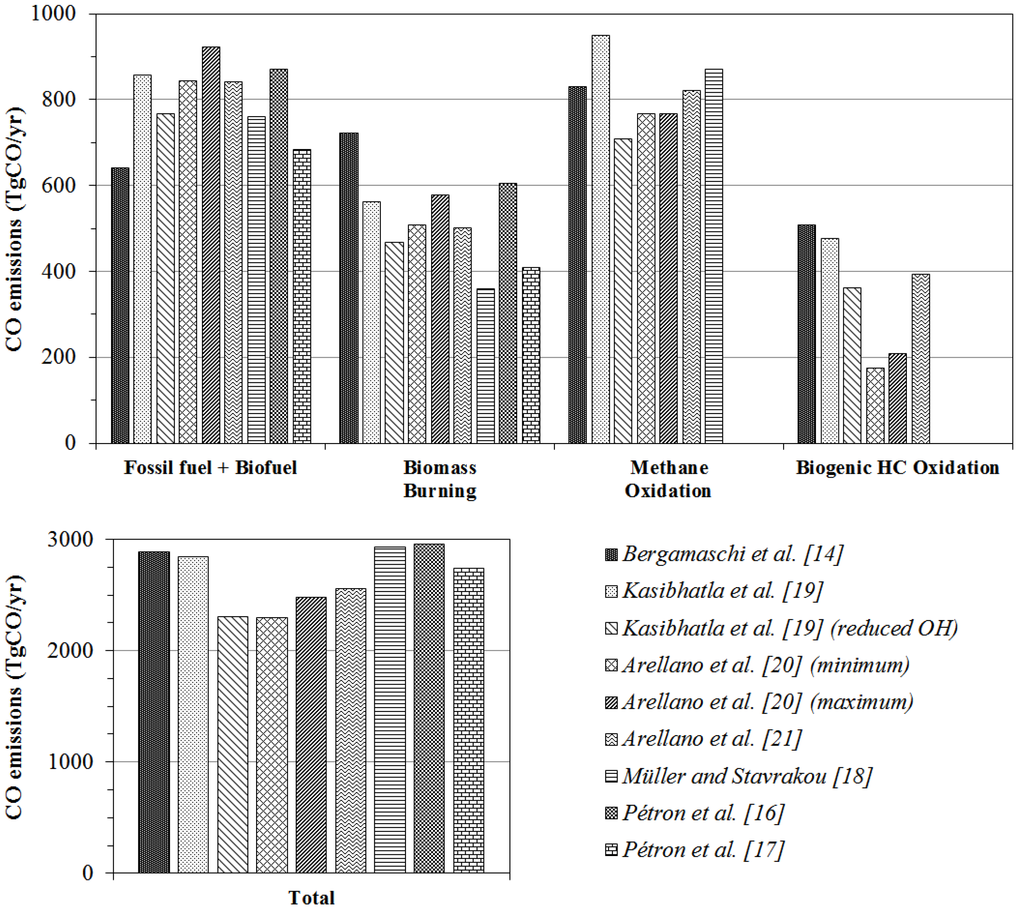
Figure 1. Carbon monoxide (CO) sources and total amount of CO emissions derived from inversion analyses.

Figure 1. Carbon monoxide (CO) sources and total amount of CO emissions derived from inversion analyses.

Figure 2. Isotopic source signatures of CO based on data in Table S2. The size of each circle represents the relative source strengths estimated in IPCC 2001 report.

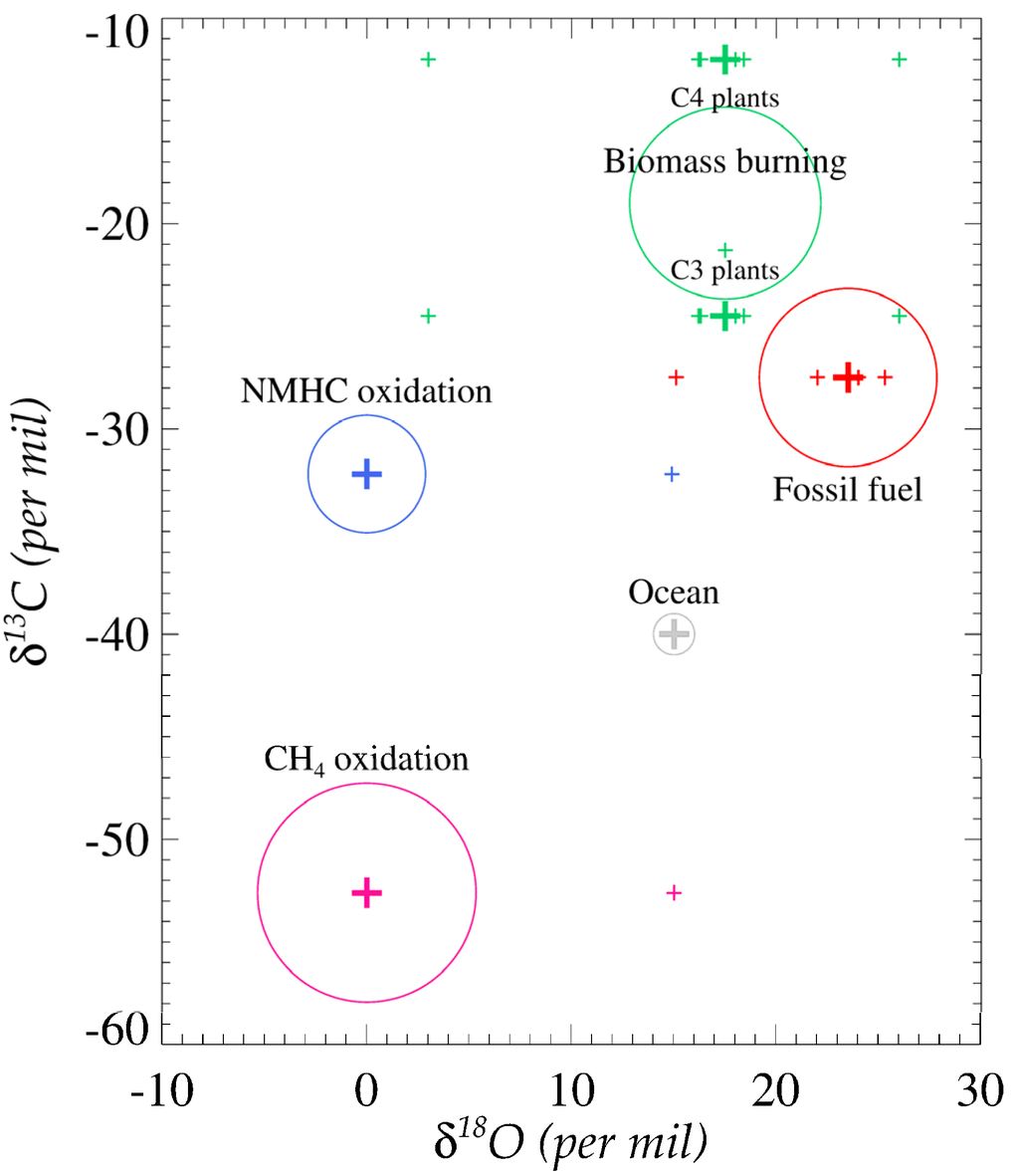
Figure 2. Isotopic source signatures of CO based on data in Table S2. The size of each circle represents the relative source strengths estimated in IPCC 2001 report.

Including isotope information in an inversion study can lead to more accurate and precise source strength estimates [28], since isotope measurements provide significant additional information on the sources by enabling separate analyses of C¹⁶O and C¹⁸O, instead of CO alone. There have been several concentration-isotope ratio inversion schemes that were applied to find the best source strength estimates of atmospheric CO₂ and CH₄ [24,26,29,30,31,32]. For carbon monoxide, Bergamaschi et al. [24] analogously adopted the methane isotope inversion technique [33] and showed isotope information can constrain the CO sources more reliably. Along with a posteriori concentration, a posteriori isotope ratio also provides additional information to confirm the inversion results and this adds more reliability to the inversion results.

The goal of the work presented here is to improve and develop a new joint inversion method of CO and its isotopes for accurate CO budget estimation. Thus, optimization methods that maximize the benefit of including isotope information are investigated. The availability of an enhanced 3-D global chemical transport model and updated isotope ratio measurements enables more robust CO inversion results. Here we use MOZART-4 (Model for OZone And Related chemical Tracers) [34] to simulate CO and δ¹⁸O in ways which agree fairly well with observations. Although, we ran the model for CO concentration and δ¹⁸O from 1996 through 2004, the availability of isotope measurements allows us to constrain CO budgets for 1997, 1998, and 2004.

For constraining the sources of CO, although the δ¹³C signature from the methane oxidation is clearly different from the other sources, this source is relatively well known. In addition, δ¹³C signatures are close to each other for some major sources (e.g., NMHC oxidation and fossil fuel use) while the oxygen isotopic source signatures are distinctly different for those sources. Therefore, this study focuses on the oxygen isotopes of CO and shows these have a greater potential to separate the CO sources [1,35,36].

The outline of the paper is as follows. The measurements of carbon monoxide concentration and its isotope ratios measurements used in this study are described in Section 2. In Section 3, detailed descriptions of the forward model simulation including inventories of a priori sources, methods of C¹⁸O incorporation, and evaluations of model performance are presented. Next, the development of various joint inversion schemes combining concentration and isotope ratio information are presented (Section 4). In Section 5, the results of inversion analyses including the source strength estimates are discussed.

2. Observation of Atmospheric Carbon Monoxide and Its Isotopes

The concentration and isotope ratios of CO used here have been measured from eight stations and most air samples were collected weekly or biweekly. The location of each station is shown in Figure S1. Table S3 shows the periods of model simulation, CO, δ¹³C and δ¹⁸O observations at each sampling location. Monthly averaged concentration and isotope ratios were used in the inversion analyses. A subset of the NOAA (National Oceanic and Atmospheric Administration) GMD (Global Monitoring division) network CO mixing ratios [37,38] was also used to get inversion results for comparison. Each concentration and isotope ratio data set was inverted individually or together to update CO source strengths.

Because the average lifetime of tropospheric CO is approximately two to three months [39], the background CO can be considered zonally well-mixed in the atmosphere and its inter-hemispheric mixing is quite limited [16,40]. Thus, sampling locations were carefully selected to represent the background state of the atmosphere at specific latitude zones.

The methodologies of the sampling and measurement techniques are well described in [41,42,43]. A brief description of the isotope analysis method is given here. The collected air samples are processed through a cryogenic vacuum extraction line. Water vapor and most trace gases are trapped in the first two cryogenic traps and CO is then oxidized to CO₂ by Schütze reagent [44]. The produced CO₂ is collected in the last cryogenic trap. Concentrations are determined by measuring the total pressure of the oxidized CO in a calibrated volume, and isotopes are measured in an isotope ratio mass spectrometer. The manometrically measured CO mixing ratios are consistent with the NOAA GMD CO measurements (Figure 3). Additionally, the National Institute of Water and Atmospheric Research (NIWA) data sets used gas chromatography method as well for quality control. The δ¹⁸O of CO₂ is converted to the δ¹⁸O of CO and the precision of measurement is ±2 ppbv for concentration, ±0.2‰ for δ¹³C and ±0.8‰ for δ¹⁸O [36,41].

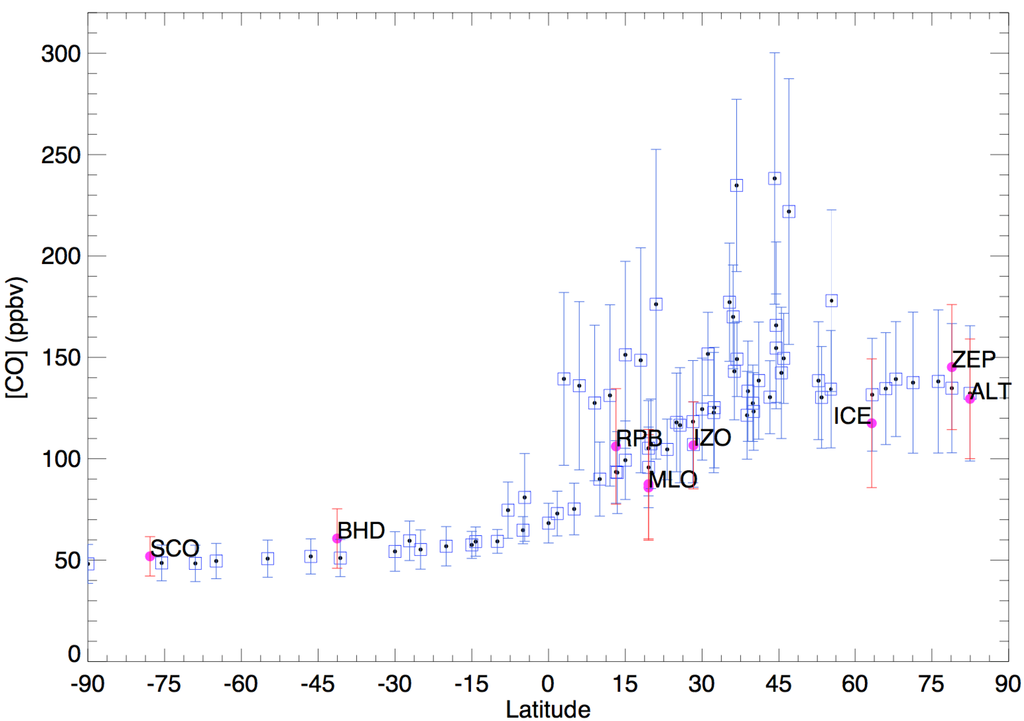
Figure 3. Global zonal distribution of CO concentration. The blue squares are National Oceanic and Atmospheric Administration Global Monitoring Division (NOAA GMD) CO and the red dots are CO used in this study, showing they are comparable. All available monthly mean concentrations during 1996–2004 are used for plotting. The error bar is the range of mean seasonal variation of the multi-year CO observations.

Figure 3. Global zonal distribution of CO concentration. The blue squares are National Oceanic and Atmospheric Administration Global Monitoring Division (NOAA GMD) CO and the red dots are CO used in this study, showing they are comparable. All available monthly mean concentrations during 1996–2004 are used for plotting. The error bar is the range of mean seasonal variation of the multi-year CO observations.

3. Forward Model Description

3.1. MOZART-4 and Its Tracer Version

MOZART-4 is a 3-dimensional global chemical transport model handling 97 chemical and aerosol species with more than 196 chemical reactions. In past studies, MOZART-4 reproduced certain observations fairly well for CO [45], ozone [46], nitric acid [47], aerosol optical depth [48], and isoprene [39]. MOZART-4 has also shown good agreement with other model simulations of CO [49] and O₃ [50].

A tracer version of MOZART-4 [34,39,51] was developed and applied in this study. Chemical reactions directly related to CO are included in the model along with prescribed mixing ratios and other parameters such as OH concentration and chemical production rates. This information is pre-calculated and saved from the simulation of a full-chemistry version of MOZART-4. Due to its simplified chemistry, the tracer version is much faster than the regular version of MOZART-4, yet still allows for analyzing the relationships between sources and concentrations or isotope ratios. In the tracer version of MOZART-4, we tagged CO for each source, isotopologue, and geographic regions of origin, which enables tracking the CO and its isotopes. Fossil fuel use, biofuel use, and biomass burning sources were divided into nine emission regions: North America, Central America, South America, North Asia, South Asia, Australia, Europe, North Africa, and South Africa. Hence, 62 tagged tracers are included in the model.

The MOZART-4 simulation used in this study has a horizontal resolution of 2.8° × 2.8°. There are 28 levels from the surface to the top of the stratosphere (2hPa). The model was driven by the NCAR reanalysis of the National Centers for Environmental Prediction forecasts (NCEP/NCAR reanalysis) [52,53]. The chemical species react and are transported in the model every 20 min. The time period of model simulation was from April 1996 to December 2004, and the first six months’ simulations were discarded since those months were considered as spin-up months.

3.2. Sources and Sinks of Atmospheric CO

The global budget of a priori CO sources used in this study is shown in Table 1. Carbon monoxide emissions from fossil fuel and biofuel use are taken from [17]. They derived CO source strengths from April 2000 to March 2001 using MOPITT (Measurement of the Pollution in the Troposphere) satellite observations and updated the inventory monthly for 15 regions. In Figure 1, some previous fossil fuel and biofuel CO inventories are shown and a priori fossil fuel and biofuel used in this study (679 TgCO/year) is a little lower than the average (799 TgCO/year).

The Global Fire Emissions Database (GFED) version 2 [54] inventory is used for the biomass burning source of CO. Annual CO emissions estimated by the GFED-v2 are shown in Table 1.

Carbon monoxide is also directly emitted from other natural sources: vegetation and the ocean. Carbon monoxide emissions from live or dead plant matter are from the photodegradation or photooxidation of cellular material [55] and oceanic CO is mainly produced by the photochemical oxidation of dissolved organic matter [56,57]. The inventories of these natural sources are taken from the POET atmospheric gas inventory [58] (Table 1).

Methane-derived CO is the most accurately constrained CO source because of the long lifetime of CH₄ (~10 years) [34,36,59,60], known atmospheric concentration, and well-known oxidation rate. Carbon monoxide from methane oxidation is calculated on-line using methane distributions specified by the zonal average of the monthly mean NOAA GMD surface CH₄ measurements.

In the tracer version of MOZART-4, NMHC-derived CO is calculated by subtracting on-line calculated methane-derived CO from the CO from total hydrocarbon oxidation taken from the full chemistry MOZART-4 runs.

Table 1. Annual mean of a priori source strengths used in this study (TgCO/year). Global Fire Emissions Database version 2 (GFED-v2) inventory is used for biomass burning carbon monoxide (CO).

Sources	Northern Hemisphere	Southern Hemisphere
Fossil fuel	340	25
Biofuel	276	38
NMHC oxidation	310	232
Methane oxidation	497	379
Ocean	8	12
Biogenic	104	57
Biomass burning (year)
1997	192	364
1998	397	193
1999	221	171
2000	199	137
2001	193	171
2002	222	196
2003	235	161
2004	192	212

Table 1. Annual mean of a priori source strengths used in this study (TgCO/year). Global Fire Emissions Database version 2 (GFED-v2) inventory is used for biomass burning carbon monoxide (CO).

Sources	Northern Hemisphere	Southern Hemisphere
Fossil fuel	340	25
Biofuel	276	38
NMHC oxidation	310	232
Methane oxidation	497	379
Ocean	8	12
Biogenic	104	57
Biomass burning (year)
1997	192	364
1998	397	193
1999	221	171
2000	199	137
2001	193	171
2002	222	196
2003	235	161
2004	192	212

Reaction with the hydroxyl radical is the dominant sink of tropospheric CO. The calculated lifetime of methane from the MOZART-4 run is 10.5 years [34] and previous estimates of 9.4 years [59] indicate that the model may slightly underestimate globally averaged OH. Another minor CO sink is its surface deposition, which is controlled by the activity of microorganisms in the soil. The soil uptake velocity is a function of soil moisture content of different ecosystems and is implemented in MOZART-4 [34,61].

3.3. Incorporation of Oxygen Isotopes

To analyze the oxygen isotopes of CO in the model, each source of CO was determined for C¹⁶O and C¹⁸O and specific chemical reaction rates and deposition velocities were assigned to each isotopologue. To build inventories of CO isotopes, for the direct emission sources, the total CO inventory is divided based on δ¹⁸O source signatures.

Both isotopologues of carbon monoxide are produced from the CH₄ + OH reaction in the model:

$$C{H}_4+OH\to 0.99799882\times C^{16}{O}_{methane}+0.00200118\times C^{18}{O}_{methane}$$

(2)

where the coefficients of the products are the relative abundance of C¹⁶O and C¹⁸O for δ¹⁸O = 0‰.

Oxidation reactions of each isotopologue are individually treated in the model since isotopic fractionation occurs during the CO + OH reaction due to kinetic isotope effects (KIE). In the model, the KIE is considered as the ratio of reaction rate constant of each isotopologue: KIE(δ¹⁸O) = k(C¹⁶O)/k(C¹⁸O) where k(C¹⁶O) and k(C¹⁸O) represent the reaction rate constants of C¹⁶O + OH and C¹⁸O + OH respectively. When CO is oxidized by the hydroxyl radical, the behavior of C¹⁸O shows an inverse mass dependence. Thus, C¹⁸O is preferentially removed from the atmosphere (KIE = 0.990) and this is weakly dependent on pressure. The rate constant for CO + OH itself is strongly dependent on pressure [62,63]. The reaction rate (k) of the CO + OH reaction and the reaction rate ratio (η) between C¹⁶O and C¹⁸O are as follows:

$$\begin{array}{l}{k}_{CO+OH}=1.5\times {10}^{-13}\times (1+0.6\times p[\text{atm}])\\ \eta {({\delta }^{18}O)}_{CO+OH}=(KIE-1)\times 1000\\ =-11.6+0.0042p-1.9\times {10}^{-6}{p}^2\end{array}$$

(3)

Carbon monoxide removal from soil uptake is similar to the normal KIE and the fractionation has been measured as η(δ¹⁸O)_{soil sink} = 12‰ [64].

The isotopic source signature from fossil fuel combustion applied in this study is 23.5‰ [42,65]. Based on Brenninkmeijer [42] and Brenninkmeijer and Röckmann [10], 0‰ is used for δ¹⁸O in CO from methane and NMHC oxidation sources. Since two globally averaged estimates of δ¹⁸O in CO from biomass burning have been reported (16.3‰ [42] and 18‰ ± 1‰ [62]), a rough average of the estimates (17.5‰) is applied in the forward model. For the ocean source of CO, 15‰ is used in the model [66].

Since there is no previous study on the δ¹⁸O of biogenic CO and biofuel CO (Table S2), δ¹⁸O values from those sources are estimated in this study. δ¹⁸O of CO from the direct biogenic emission was estimated to be 0‰. While the factors controlling this source are not well known [67], it is a minor source of CO (60–160 TgCO/year) [1]. Thus, uncertainties originated from this assumption should not largely affect the modeled results. The isotopic source signature from biofuel use is assumed to be the same as δ¹⁸O of CO from biomass burning.

3.4. Simulated Atmospheric [CO] and δ¹⁸O: Model Evaluation

Because an inverse modeling method relies on the assumption that the physical-chemical connection between the parameters (e.g., source strengths and reaction constants) and the observed properties (e.g., concentration and isotope ratio) are known, if a chemical transport model does not simulate the real measurement accurately, its source estimates would lose reliability even though all of the mathematical assumptions are correct. To get more confidence in our forward modeling results, NOAA GMD CO concentrations are shown together in Figure S2.

Three different measures are used here to assess the model performance: chi-squared (goodness of fit) test, model-observation difference and correlation. Usually the “correlation” represents dissimilarity of the trend or patterns between the modeled property and measured property and the “distance” shows the offset between the model and measurements. If a model accurately reproduces observational data, the distance (d) will be close to ‘0’ and correlation (ρ) will be close to “1”. The goodness of fit of a model statistically describes how well a simulated result fits the measured data set. The reduced chi-square (χ_red²) is chi-square divided by the number of degrees of freedom and this estimates the ratio of the variance of modeled data set to the variance of measured data set. If the observed data are well explained by the model, the χ_red² value will be close to 1.

The results of the evaluation at each station are shown in Table S5. For the overall data sets, the modeled and measured concentration showed a strong correlation (ρ = 0.94) which implies the model captures the seasonal and interannual variation of the CO sufficiently and the mean model-observation difference was 10.5 ppbv. Figure 4 shows Southern Hemispheric (SH) CO concentrations are slightly overestimated by the model (SCO: 6.2 ppbv, BHD: 6.4 ppbv). This possibly results from the underestimation of OH or overestimation of some sources. However, if OH is increased, the modeled δ¹⁸O will be smaller and therefore further removed from the 1:1 correlation line (Figure 4). Hence, to fit both δ¹⁸O and CO, the strength of sources having a light δ¹⁸O signature (oxidation sources) should be reduced.

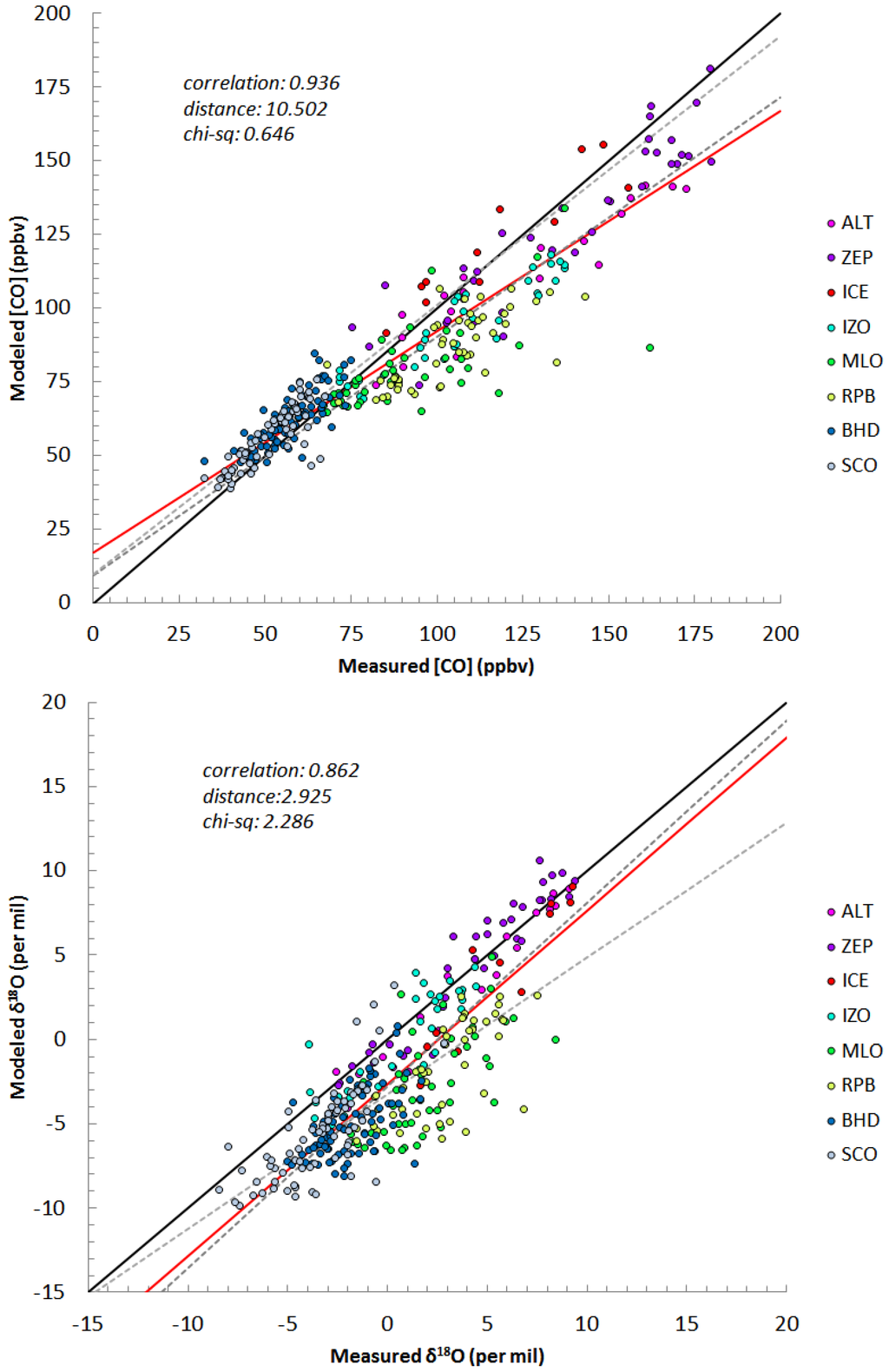
Figure 4. A scatter plot of measured versus modeled concentration of CO (upper panel) and measured versus modeled δ¹⁸O of CO (lower panel). The black solid line depicts 1:1 correspondence and the red line is a regression line of all measurements. The dotted lines are regression lines of the NH (dark gray) and the SH (light gray) data sets.

Figure 4. A scatter plot of measured versus modeled concentration of CO (upper panel) and measured versus modeled δ¹⁸O of CO (lower panel). The black solid line depicts 1:1 correspondence and the red line is a regression line of all measurements. The dotted lines are regression lines of the NH (dark gray) and the SH (light gray) data sets.

Since the NMHC oxidation source has a strong seasonality (Figure S3), even if the source strengths are decreased, it is not applicable to explain the year-round overestimation of the modeled CO concentration. In Manning et al. [35], they estimated CO yield from the CH₄ oxidation is less than 0.7 based on δ¹³C measurements while 1 is used for the yield in this study which is also assumed in Duncan et al. [68]. This suggests the presented CH₄ oxidation source might be overestimated in the SH. In the NH, especially during the winter, modeled concentrations are generally lower than measured concentrations (Figure 4). For δ¹⁸O, the model accurately reproduced observations at high latitude stations (ICE, ZEP, ALT) while the modeled δ¹⁸O were lighter than the observations at mid- and low latitude stations. In high latitudes, the dominant sources (fossil fuel and biofuel combustion) have isotope ratios that are similar to the mean isotope ratios of total CO. Thus, the isotopic data is not sensitive to their source strength change, particularly during winter. For example, the wintertime oxygen isotope ratio from the biofuel source in high latitude is approximately 12‰ and total δ¹⁸O‰ (shown in Figures S3 and S4 respectively), so variations in this source have a minimal effect on δ¹⁸O but can improve the concentration fit. In the mid- and low latitude NH, the underestimations of the modeled [CO] and δ¹⁸O implies that the ¹⁸O enriched sources (fossil fuel, biofuel and biomass burning) are underestimated in the model.

The χ_red² of the forward model run for CO concentration was 0.65 and of δ¹⁸O was 2.29. The modeled δ¹⁸O shows good agreement to measurements, however, the simulation results of CO concentration were even more reliable; ρ_[CO] = 0.94 > ρ_δ18O = 0.86 and χ_red²_[CO] = 0.65 < χ_red²_δ18O = 2.29. This supports the discrepancies of global CO source distributions of previous studies shown in Figure 1; the current estimation of total CO emission is relatively well defined, whereas the strength of each source is less certain. The δ¹⁸O signatures of natural sources such as biomass burning and NMHC oxidation have more variability and uncertainty which might lead to additional errors in the isotope simulation.

4. Methodology for Inverse Modeling Analysis

4.1. Bayesian Synthesis Inversion

The Bayesian inversion method was used to find the best estimates of source strengths of CO. Assuming a Gaussian distribution for all probability distributions and a linear relationship between sources and concentrations [14,16,18,20,21,24], the measured concentration of CO can be expressed as:

$$y=Kx+e$$

(4)

where y is the observed concentrations of CO, x is the vector of each CO source strength, K is the Jacobian matrix that links concentration and source strength calculated from the forward chemical transport model and e is the total error of measurement and model. Since K describes the sensitivity of CO concentration to the source change, Kx represents a modeled concentration of CO that expressed itself as a sum of the concentration of each source category.

The maximum a posteriori (MAP) probability solution of the inverse problem is finding an $\widehat{x}$ ($\widehat{x}={\displaystyle \int xP(x|y)dx}$) where the posteriori probability distribution is a maximum, i.e.,

$$\widehat{x}=x_a+(K^T{S}_e^{-1}K+S_a^{-1}{)}^{-1}{K}^T{S}_e^{-1}(y-K{x}_a)$$

(5)

X_a denotes a matrix of a priori source strength estimates, S_e is the error covariance matrix of the model, S_a is the error covariance matrix of prior information and $\widehat{x}$ is a matrix of optimized source strengths. The covariance matrix of $\widehat{x}$ is expressed as:

$$\widehat{S}=(K^T{S}_e^{-1}K+S_a^{-1}{)}^{-1}$$

(6)

4.2. Assigning Uncertainties in the Analyses

Two error covariance matrices are involved in the inversion calculation using the Bayesian method. Properly specifying and assigning those uncertainty terms is a particularly important part of the analysis since both inversion results and the a posteriori error covariance matrix (Ŝ) can be sensitive to the error covariance matrices [28,69].

4.2.1. Uncertainties in Measurements: S_e

The total observations error (S_e) is a diagonal covariance matrix comprised of the following uncertainties: measurement error, representation error, and forward model error.

$$e_{observation}=\sqrt{e_{measurements}^2+e_{representation}^2+e_{forwardmodel}^2}$$

(7)

The measurement error is the sum of all factors affecting the accuracy of the measurement including instrumentation error, CO extraction system error, and inter-calibration error. Brenninkmeijer estimated the maximum absolute uncertainty (m.a.u.) of CO concentration as 2% and of δ¹⁸O as 1‰ [42]. The same extraction system design for analyzing CO concentration and measuring isotope ratios are used in this study. The errors of measurements presented here (1 σ) are calculated to be 1.3% and 0.27‰, respectively, through the more than 300 calibration runs. Therefore, the m.a.u. of our data sets is also conservatively estimated as 2% for concentration. Since, for δ¹⁸O measurements, the systematic error produced from the Schütze oxidant is dominant and is less than 1‰, the m.a.u. is estimated at 1‰ (Table 2) [41,42].

Table 2. Estimated and measured uncertainties in isotopic and concentration measurements.

Quantity	Unit	Uncertainty (1σ)		e.m.a.u *
		Brenninkmeijer [41]	This Study
CO	ppbv	1.70%	1.31%	2%
δ18O	‰, VSMOW	0.40‰	0.27‰	1‰

* e.m.a.u denotes estimated maximum absolute uncertainty, i.e., sum of systematic and random errors.

Table 2. Estimated and measured uncertainties in isotopic and concentration measurements.

Quantity	Unit	Uncertainty (1σ)		e.m.a.u *
		Brenninkmeijer [41]	This Study
CO	ppbv	1.70%	1.31%	2%
δ18O	‰, VSMOW	0.40‰	0.27‰	1‰

* e.m.a.u denotes estimated maximum absolute uncertainty, i.e., sum of systematic and random errors.

To apply the errors to the inversion analysis, the estimated error of CO and δ¹⁸O are converted to the error of C¹⁶O and C¹⁸O. The error of C¹⁶O is considered to be the same as that for CO. The δ¹⁸O error is converted for C¹⁸O error using both C¹⁶O error and δ¹⁸O error because, by the definition of the δ-value, δ¹⁸O is the ratio of C¹⁶O to the C¹⁸O. Thus, the total measurement error is propagated to 5.4%. Typically, in CO inversion studies, the measurement error has been evaluated as less than 2% [20,69]. However, 5.5% for the measurement error was applied here since the uncertainty of the isotope ratio is commonly higher than the uncertainty of the concentration due to the trace amount of the minor isotopes.

Because, practically, there is no ‘true’ model to measure the uncertainties of the chemical transport model, errors in forward models are very hard to quantify. Sometimes the uncertainties of the forward model are neglected and the model is assumed to be perfect [16]. In this study, the errors related to the forward model (e² _{representation} and e² _{forward model}) are treated as described below.

Representation error is an aggregated error of the mismatch of the spatial and temporal scale between the model and observation. Usually, for analyzing both concentration and isotope ratios of CO, air samples are collected for a couple of hours at a surface station while, in the model, the size of the corresponding grid box is 2.8° × 2.8° and the concentration is averaged for a day. Since the CO monitoring sites used for this inversion analysis are located in remote locations, local sources minimally affect the CO measurements. It is also assumed that CO is blended well in the atmosphere on the scale of each model grid box because the average lifetime of CO is several months. Therefore, the contribution of representation error to the uncertainty analysis is considered to be minimal. In [69], aircraft measurements in each model grid box were used to define the representation error. The variability of the direct measurements was approximately 5%–10% in each 2° × 2.5° grid. The representation error is analyzed by calculating the percentage of mean variance of monthly modeled concentration from the overall mean concentration and 8% of the concentration is obtained in this study [19,70,71].

Another uncertainty related to the model is the forward modeling error. It consists of errors raised from inaccurate or incomplete chemical reactions, transport, and model parameters (e.g., reaction rates and kinetic isotope effects). Error estimation is performed following [69], which assumed the residual of the relative error (i.e., the standard deviation of (K_a − y)/y where K_a denotes modeled concentration and y is observed concentration) represents the uncertainties of the chemical transport model. In this study, the forward modeling error was calculated to be 8.5% of the concentration.

The observation error covariance matrix S_e is derived from the sum of the measurement error and representation error and forward chemical model error. The total observation error is approximately 13%. Considering unknown and unevaluated possible error factors, 15% is used in this study for the total observation error in the inversion analyses [9,16,18,20,69,72,73].

4.2.2. Uncertainties in a Priori Source Estimates: S_a

The bottom-up estimates of CO source strengths still have large error ranges and the top-down estimates cover a wide range (Figure 1). Thus, to start with, large uncertainties are assigned to the a priori emissions, which weakly constrains the sources. In [74], the uncertainty of global annual emissions of biomass burning CO was estimated at 30%; however, they also indicated that the regional variations are often much higher (factor of 2–5). Duncan et al. [68] showed a 25% uncertainty remains for fossil fuel CO despite rigorous and extensive bottom-up estimates. The inconsistency of source estimates from the previous inversion analyses shown in Figure 1 also indicates that the uncertainty of each source is at least 20% for anthropogenic, 50% for biomass burning, 100% for biogenic hydrocarbon oxidation, and 15% for CH₄ oxidation [14,16,17,18,19,20,21]. Previous studies also carefully started inversion analyses using weak constraints: 50% of a priori source strength estimates [20,21,68,69,75]. In this study, to find the best estimate of the a priori source error covariance matrix (S_a), a sensitivity test was performed to analyze the response of inverse modeling results with varying S_a.

In Figure 5 and Figure 6, smaller optimized model-observation differences were found with higher a priori source uncertainties (S_a). However, the inversions with larger uncertainties frequently failed to constrain the sources. Not only a posteriori errors are increased after inversion for some cases but also unrealistic large source changes or negative sources are obtained. Assigning more than 100% of the uncertainties of each CO source tends to ignore the a priori information too much during the inversion process. In contrast, the inversion analyses fail to improve the a priori inventories with small uncertainties, e.g., 10% or 20%, because they significantly rely on the a priori source information rather than the observations. The distance between the measured concentration and the a posteriori concentration converged to a specific value after assigning higher than 50% of source uncertainties in the all three cases (97NH, 04SH, and 04NH in Figure 5); the inversion results are insensitive to larger than 50% error covariance matrices.

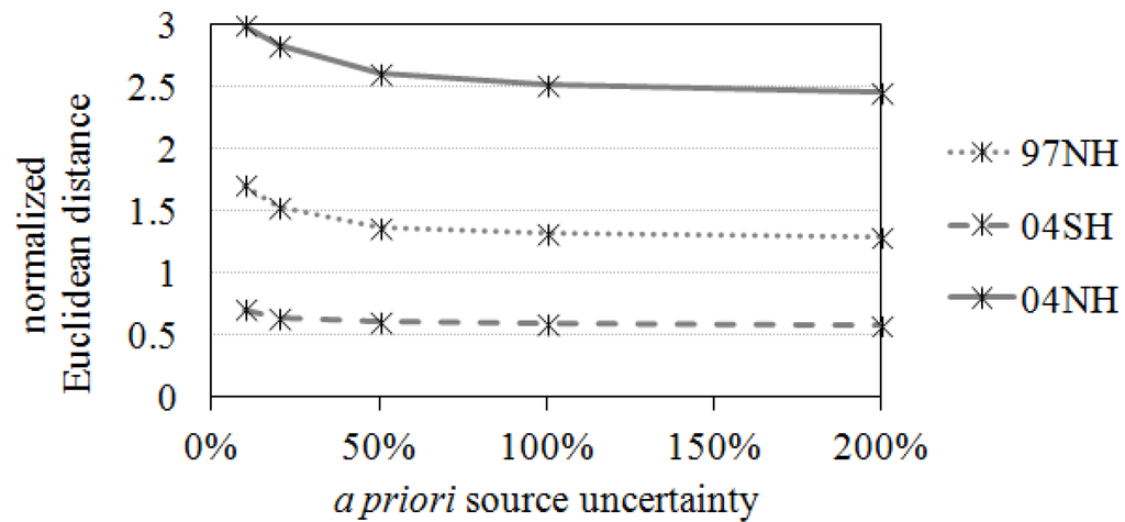
Figure 5. Averaged distance between the measurements and a posteriori CO concentrations.

Figure 5. Averaged distance between the measurements and a posteriori CO concentrations.

Figure 6. Inversion results (optimization factors and a posteriori errors) of each source with different a priori source uncertainties. A logarithmic scale is used for optimization factors.

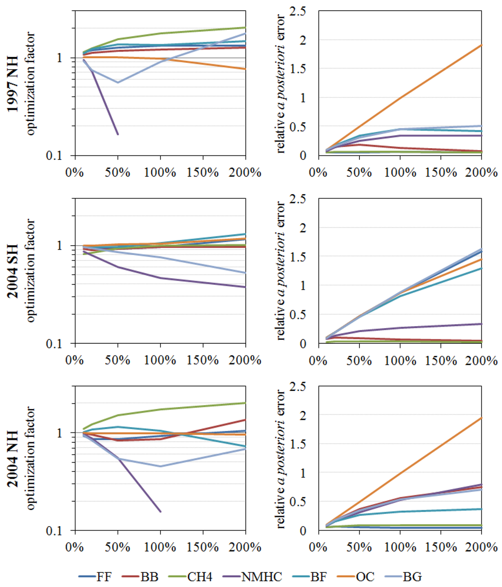
Figure 6. Inversion results (optimization factors and a posteriori errors) of each source with different a priori source uncertainties. A logarithmic scale is used for optimization factors.

Hence 50% of the current source estimates are determined to be within the most proper uncertainty range, based on our sensitivity test results and prior investigations. In addition, instead of assigning the same errors for all of the sources, additional constraints were given to the methane oxidation sources and fossil fuel sources. Because atmospheric methane has a long lifetime, its reservoir is relatively well known and only a 7% interannual variability was observed during 1978–1998 [76]. Moreover, in these model studies, the CH₄ oxidation source is directly scaled to the NOAA GMD surface measurements. Therefore, 10% is assigned for the a priori error of methane-derived CO. For the fossil fuel source, many inversion studies have been updating the fossil fuel source inventory (Figure 1) and this is relatively well known, compared to the natural sources. The a posteriori error of the fossil fuel emission inventory in [17] was evaluated as 13% for the global average, and the variability of anthropogenic source strength estimates shown in Figure 1 was 18%. Thus, 18% was defined as the maximum uncertainty and we choose 20% for the uncertainty (S_a) of fossil fuel sources, which arbitrarily added 2% to loosen the constraint (S_a). Thus, the a priori source estimation errors (S_a) are set to 10% for methane oxidation sources, 20% for fossil fuel sources, and 50% for all other sources.

4.3. Inversion Schemes; Incorporation of Isotope Information to the Source Optimization

Since the units of concentration (ppbv) and isotope ratio (‰) are different, the meanings of unity for the model-observation difference are very different and are not comparable. The impact of the different units should be correctly accounted for the inversion [77]. Previous studies [24,26,33] have solved the inverse problems through minimizing the model-observation difference without balancing the two properties.

Furthermore, for carbon monoxide, in contrast to carbon dioxide or methane, its lifetime is short and, therefore, its temporal variation is relatively large. This is especially important for C¹⁸O. For example, in the NH mid-latitude, the typical inter-seasonal variation of δ¹³C of CO is 5‰ and δ¹⁸O of CO is 8‰, while δ¹³C of CO₂ is 0.4‰ and CH₄ is 0.5‰ [36,43,78,79]. Thus, if the long-lived species’ isotope-inverting methodologies are analogously applied to the CO isotope inversion, nonlinearity problems develop and can affect the inversion results [33].

In this study, a two stage isotope inversion scheme is devised that is able to avoid the shortcomings of the previous isotope inversion methods as well as more effectively constrain the sources of CO.

4.3.1. Decoupled Inversion

The scheme of the decoupled inversion is basically an extension of the CO-only inversion that has been performed by the previous Bayesian synthesis inversion studies. While the CO-only inversion uses the concentration of CO, the decoupled inversion uses C¹⁶O and C¹⁸O separately. Since the measurement errors and model uncertainties in C¹⁶O and C¹⁸O are assumed to be uncorrelated, the sources of C¹⁶O and C¹⁸O can be individually optimized by using the C¹⁶O and C¹⁸O information:

$$\begin{array}{l}{}^{16O}\widehat{x}={}^{16O}{x}_a+{({}^{16O}K{}^{T}S_e^{-1}{}^{16O}K+S_a^{-1})}^{-1}{}^{16O}K{}^{T}S_e^{-1}({}^{16O}y-{}^{16O}K{}^{16O}{x}_a)\\ {}^{18O}\widehat{x}={}^{18O}{x}_a+{({}^{18O}K{}^{T}S_e^{-1}{}^{18O}K+S_a^{-1})}^{-1}{}^{18O}K{}^{T}S_e^{-1}({}^{18O}y-{}^{18O}K{}^{18O}{x}_a)\end{array}$$

(8)

where, ¹⁶O and ¹⁸O indicate the C¹⁶O and C¹⁸O data sets.

The two independent inversion results allow for the estimation of both a posteriori C¹⁶O and C¹⁸O source strengths. The ratio of ${}^{16O}\widehat{x}$ to ${}^{18O}\widehat{x}$ also provides a posteriori δ¹⁸O signature of the CO sources. This approach can be applied to evaluate potential correlations among isotopologues in isotope inversions.

4.3.2. Coupled (Simultaneous) Inversion

Two different joint inversion approaches that combine concentration and isotope ratio data sets were tested in this study. One is a simultaneous inversion technique, where the concentration and isotope information constrain the sources in one inversion process. The other is a sequential inversion technique: each of the measured properties constrains the sources in two consecutive inversion processes.

In the simultaneous inversion, both modeled and observed concentration and isotope ratio are coupled in the solution matrices for the inverse problem:

$$\widehat{x}=x_a+\left({\left[\begin{array}{c}{}^{16O}K\\ {}^{18O}K\end{array}\right]}^T{S}_e^{-1}\left[\begin{array}{c}{}^{16O}K\\ {}^{18O}K\end{array}\right]+S_a^{-1}\right){\left[\begin{array}{c}{}^{16O}K\\ {}^{18O}K\end{array}\right]}^T{S}_e^{-1}\left(\left[\begin{array}{c}{}^{16O}y\\ {}^{18O}y\end{array}\right]-\left[\begin{array}{c}{}^{16O}K{}^{16O}{x}_a\\ {}^{18O}K{}^{18O}{x}_a\end{array}\right]\right)$$

(9)

Since the two measurement data sets (major and minor isotopes; C¹⁶O and C¹⁸O) are used to optimize the sources at the same time, the isotope information plays like an additional observational data set in the inversion system and, in comparison with the [CO]-only inversion, this renders more robust inversion results.

4.3.3. Coupled (Sequential) Inversion

When simultaneously inverting different data sets that have a large difference in their magnitude (e.g., C¹⁶O and C¹⁸O), a weighting issue arises because the inversion results can be dominantly constrained by the larger magnitude measurement data. One of the methods to balance the contribution of two data sets is sequential use of each observation, where the solution inverts one measurement data set first and the result provides the input for the inversion of the second observational information [77,80].

In this study, the sequential use of concentration and isotope information is formulated as follows:

$$\begin{array}{l}\text{step\hspace{0.17em}1:\hspace{0.17em}\hspace{0.17em}\hspace{0.17em}}{x}^{*}=x_a+{({}^{16O}K{}^{T}S_e^{-1}{}^{16O}K+S_a^{-1})}^{-1}{}^{16O}K{}^{T}S_e^{-1}({}^{16O}y-{}^{16O}K{x}_a)\\ \text{step\hspace{0.17em}2:\hspace{0.17em}\hspace{0.17em}\hspace{0.17em}}\widehat{x}=x^{*}+{({}^{18O}K{}^{T}S_e^{-1}{}^{18O}K+S_a^{-1})}^{-1}{}^{18O}K{}^{T}S_e^{-1}({}^{18O}y-{}^{18O}K{x}^{*})\end{array}$$

(10)

where x^* is an intermediate estimated source strength vector that is acquired from the first step of the inversion process.

The joint inversion results of the simultaneous use of concentration and isotope ratios and the sequential use of them are compared and discussed in detail in Section 5.3.

4.3.4. Optimization of Source Strengths and δ¹⁸O Signature in These Inversion Methods

Estimating the fluxes of each CO source by jointly inverting C¹⁶O and C¹⁸O is the primary purpose of this study. In addition to this, C¹⁸O source strength estimates are derived from the optimized CO source strengths and a posteriori isotope ratio (r_j) of each source obtained from the decoupled inversion (Figure 7). Although the same prescribed isotopic source signatures can be applied to calculate a posteriori isotope ratios, Bergamaschi et al. [24] showed that applying a posteriori carbon isotopic source signatures, instead of using fixed isotopic source signatures, provides more robust inversion results. Our comparison of the inversion results with fixed and updated oxygen isotopic source signatures confirm their result for the oxygen isotopic source signatures (Section 5). Thus, the δ¹⁸O source signature optimization process is implemented in the joint inversion system, in lieu of assuming fixed isotope ratios of the sources. Optimized δ¹⁸O source signatures calculated from the a posteriori CO and C¹⁸O source strengths provide an additional benefit of including isotopic signatures in inverse modeling. It allows for the verification of the joint inversion results by showing the fit of the optimized δ¹⁸O values to the observations, while the CO-only inversions can confirm the results only by comparing measurements with a posteriori CO concentrations.

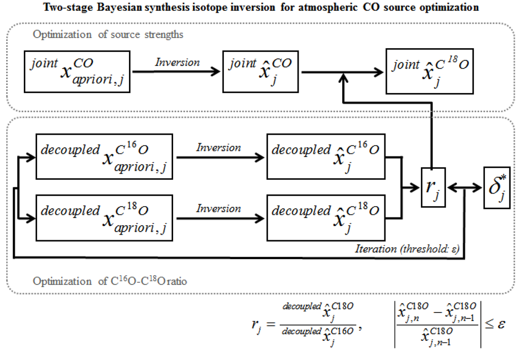
Figure 7. Schematic diagram for the two-stage Bayesian synthesis isotope inversion for atmospheric carbon monoxide.

Figure 7. Schematic diagram for the two-stage Bayesian synthesis isotope inversion for atmospheric carbon monoxide.

To optimize the isotopic source signature, the C¹⁶O-C¹⁸O ratio is iteratively optimized from the decoupled run since it has been known that the isotope ratio is a nonlinear function of the source strengths [24]. Therefore, an iterative method that updates the Jacobian matrix (K, Equation (4)) in each iteration was used to solve the inverse problem (Figure 7). Iterations were performed for each source and continued until the solution converged:

$$\left|\frac{{\widehat{x}}_{j,n}^{C18O}-{\widehat{x}}_{j,n-1}^{C18O}}{{\widehat{x}}_{j,n-1}^{C18O}}\right|\le \epsilon$$

(11)

During the iterations, the isotope ratios were allowed to vary within a certain range (ε). The threshold is assigned for each source based on current understanding of the isotopic source signature. For the fossil fuel source, 2‰ is assigned for the threshold since the previous estimates of the isotope signatures are reported in between 22‰ and 24‰ [10,42,62,65] and the direct measurements of the exhaust from numerous automobiles indicate the variations of δ¹⁸O of CO as ±1.0‰ [81]. The previous global estimates of δ¹⁸O from biomass burning were 16.3‰ and 18‰ [42,65] and the uncertainties reported for biomass burning source signature were ±1‰ [62,82]. However, 5‰ is allocated for the threshold of the biomass burning source because [83] indicated a very wide range (3‰–26‰) for δ¹⁸O from their chamber experiment. For the ε of the other sources, since there is one number reported for δ¹⁸O of the sources, ±5‰ is estimated for ε, analogous to that for the biomass burning source.

The role of isotope information is expanded in the inverse modeling analysis with the optimized source signatures. This enables the separation of the a posteriori source estimates to the inventories of major and minor isotopes while the joint inversion gives updated information of the CO source strengths.

5. Optimized Global CO Budget from Joint Inversion of [CO] and δ¹⁸O

5.1. Optimized Atmospheric CO Sources for 1997, 1998, and 2004

The global atmospheric CO budget is estimated for 1997, 1998 and 2004. The sources are constrained by both CO concentration and oxygen isotope ratio information. Concentration and δ¹⁸O are either simultaneously or sequentially applied to constrain the a priori CO sources and the former method is used to discuss the inversion results, unless otherwise noted. The results of applying different inversion techniques will be explained in detail later in this section.

Frequently, the result of inversion analysis is expressed as a correction or optimization factor (f) that is the ratio of a posteriori estimates to the prescribed a priori source fluxes.

$$f_i=\frac{{\widehat{x}}_i}{x_{a,i}}$$

(12)

where x_a and $\widehat{x}$ is a priori and a posteriori source strength of source i. Thus, if an optimization factor is greater than 1, then this means the current estimate of source strength is underestimated.

Table 3. Optimization factors (f) and a posteriori uncertainty (e, %) of each CO source.

		Fossil fuel		Bio. burn.		CH4 ox.		NMHC ox.		Biofuel		Ocean		Biogenic
		f	e	f	e	f	e	f	e	f	e	f	e	f	e
NH	1997	1.10	1.7	1.33	8.8	1.12	0.8	0.72	7.8	1.79	12.6	1.05	24.9	0.53	15.1
	1998	0.98	2.3	0.89	4.0	1.11	0.8	1.48	9.1	1.64	12.5	1.06	24.9	0.79	20.0
	2004	0.87	1.6	0.94	18.4	1.10	0.8	1.07	9.4	1.31	10.9	1.00	24.9	0.47	16.9
SH	1997	0.98	4.0	0.97	7.5	0.97	0.6	0.67	7.0	0.86	23.0	0.96	22.2	0.79	23.1
	1998	1.00	4.0	0.75	6.9	0.98	0.7	0.85	7.8	1.01	23.8	0.98	22.4	0.99	23.0
	2004	0.99	4.0	0.93	4.7	0.98	0.7	0.52	6.5	0.96	23.1	0.98	22.5	0.84	23.0

Table 3. Optimization factors (f) and a posteriori uncertainty (e, %) of each CO source.

		Fossil fuel		Bio. burn.		CH4 ox.		NMHC ox.		Biofuel		Ocean		Biogenic
		f	e	f	e	f	e	f	e	f	e	f	e	f	e
NH	1997	1.10	1.7	1.33	8.8	1.12	0.8	0.72	7.8	1.79	12.6	1.05	24.9	0.53	15.1
	1998	0.98	2.3	0.89	4.0	1.11	0.8	1.48	9.1	1.64	12.5	1.06	24.9	0.79	20.0
	2004	0.87	1.6	0.94	18.4	1.10	0.8	1.07	9.4	1.31	10.9	1.00	24.9	0.47	16.9
SH	1997	0.98	4.0	0.97	7.5	0.97	0.6	0.67	7.0	0.86	23.0	0.96	22.2	0.79	23.1
	1998	1.00	4.0	0.75	6.9	0.98	0.7	0.85	7.8	1.01	23.8	0.98	22.4	0.99	23.0
	2004	0.99	4.0	0.93	4.7	0.98	0.7	0.52	6.5	0.96	23.1	0.98	22.5	0.84	23.0

5.1.1. Optimized Fossil Fuel and Biofuel Source Strength

While fossil fuel and biofuel are both anthropogenic sources of CO, the inversion analysis showed very different results (Table 3). In the SH, the optimization factors of fossil fuel and biofuel sources are close to unity. This implies that the anthropogenic sources of CO in the SH were accurately estimated. The fossil fuel source changed less than 2% after inversion and biofuel estimates changed less than 5% except in 1997, during which the a posteriori biofuel source decreased 15%. Since the anthropogenic sources play a minor role in the SH, the measurements did not constrain the sources tightly. The reductions of their uncertainties are relatively small compared to those in the NH where the sources are major components of total CO concentration.

In the NH, the optimized fossil fuel emission inventory was adjusted less than approximately ±15% for the three years. This indicates the a priori fossil fuel source strength [17] is close to the actual fossil fuel CO emission in both hemispheres. A slight decreasing trend of the optimization factor is also found suggesting CO emissions from fossil fuel combustion decreased from +10% (1997) to −13% (2004), albeit a 20% increase in annual global fossil fuel consumption from 1990 to 2005 [World Resources Institute, http://earthtrends.wri.org]. This may reflect advancement of fossil fuel use efficiency and stricter regulations for vehicle emissions. The NH biofuel emission changed significantly after the inversion. It increased 79% in 1997, 64% in 1998, and 31% in 2004. In comparison with the fossil fuel source, the biofuel source showed a larger source adjustment with a larger a posteriori error covariance. This indicates that there are large uncertainties in biofuel source estimate. The biofuel source also demonstrated a downward tendency of the optimization factor, which indicates the use of biofuel decreased from 1997 to 2004.

5.1.2. Optimized Biomass Burning Source Strength

There was only a small difference between the a priori and a posteriori source strengths for biomass burning in 1998 and 2004; however, for 1997, which was a high fire year, the inversion results suggest an increase of 33% for the NH biomass burning CO indicating GFED-v2 missed some sources of the biomass burning CO. The inventory was also not adjusted much for the SH biomass burning CO. In general, the joint inversion analyses estimated ca. 10% less CO than the GFED-v2 inventory on average.

5.1.3. Optimized Chemical Oxidation Source Strengths

The methane oxidation source is the biggest source of CO. However, because the methane lifetime is long (~10 years) and its reservoir is large, this source is already relatively well-constrained compared to the other sources of CO. The joint inversion analysis confirmed this. For all three years, the optimization factors are relatively constant in each hemisphere; 1.10–1.12 in the NH and 0.97–0.98 in the SH.

Biogenic NMHC emission is the largest component of the NMHC oxidation source of CO (>80% of total NMHC-derived CO; [14,68]). Isoprene emissions are estimated to be ~75% of the total natural NMHC emissions [39]. Therefore, this source is expected to be sensitive to environmental factors such as temperature and precipitation patterns. The strong El Niño event in 1997 was followed by a strong La Niña in 1998–1999 and the effect of this on the NMHC-derived CO source is seen very clearly in the inversion analysis for each hemisphere. NMHC-derived CO also responded more sensitively to the ENSO index change in the NH [84].

5.1.4. Optimized Ocean and Biogenic Source Strengths

The optimization factors of the ocean source were close to 1 and a posteriori uncertainty was not reduced much. Thus, this source was hardly constrained because of the small influence of the ocean on the atmospheric CO.

The inversion results of direct biogenic CO emission sources suggest a reduction of the emission by up to 50%. However, due to the small contribution of the biogenic source, it has limited influence to the global CO. Similar to the ocean source, this also was not tightly constrained as evidenced by a small reduction in the uncertainty of the source.

5.1.5. Comparison to the Previous CO Sources Strength Estimates Derived from Inversion Analyses

The global CO budget estimated in this study is compared to previous CO budget estimates (Table 4). Although direct comparison between this study and earlier studies is difficult due to the different years of data sets and source categories, most of the a posteriori emissions fall within the range of the previous estimates.

The total direct CO emission was 1210–1651 TgCO/year and the total chemical production of CO was 1300–1579 TgCO/year. Those show large ranges because of the large interannual variability of biomass burning CO (direct emission) and biogenic NMHC-derived CO (chemical production). Both of the improved CO inventories are also placed within the previously reported estimated value ranges; 1091–1663 TgCO/year for direct emission and 1461–1644 TgCO/year for chemical production. The total CO emission and the individual a priori sources are mostly updated by the inversion analysis (this study) within the range of previous source estimates. Hence, isotope information adjusts each source strength more precisely and accurately while keeping consistency with the total inventory estimates.

5.2. A Posteriori CO and δ¹⁸O

In order to see the effect of updated source inventories on the CO concentration and δ¹⁸O, the difference between a posteriori CO and δ¹⁸O and observations are analyzed. A detailed derivation of a posteriori CO and δ¹⁸O is described in the auxiliary material (Doc. S1). The new source inventory is more reliable if, in comparison with the model–observation difference, which is based on the a priori source information, the difference between a posteriori source strengths derived CO and δ¹⁸O is reduced.

The model–observation differences of δ¹⁸O are apparently reduced by more than 50% when the a posteriori source strengths are applied (Figure 8 and Figure 9, Table S6). The modeled concentration also showed a better fit to the measurements with the updated source inventory (Figure 8). Although, since the forward concentration simulation already reproduced the observations quite well (Figure 4), the improvement of a posteriori CO concentration is not as clear as a posteriori δ¹⁸O (Figures S4 and S5), the modeled concentrations are about 45% closer to the observations (Figure 8). Figure S4 shows that the a posteriori inventory especially improves wintertime modeled CO. While the a posteriori source emissions are estimated for each year and do not contain seasonality, this implies certain sources are significantly underestimated during the winter. The a posteriori δ¹⁸O decreased the overall offset of model-observation difference (Figure 9) and the improvement was more noticeable in the SH (Figure 8).

Table 4. The results of global CO budget estimation (this work) in comparison to previous global CO budget estimates.

	This work				Bergamaschi et al. [14]	Petron et al. [16]	Petron et al. [17]	Muller and Stavrakou, [18]	Kasibhatla et al. [19]	Arellano et al. [20]	Arellano et al. [21]	Duncan et al. [67]
	a priori	a posteriori
Year of observational data		1997	1998	2004	1993–1995	1990–1996	Apr. 2000–Mar. 2001	1997	1993–1995	2000	Apr. 2000–Apr. 2001	1988–1997
Fossil fuel (FF)	365	397	359	321		309	365					464–487
Biofuel (BF)	313	524	489	396		561	318					189
FF + BF	678	922	849	716	642	870	683	760	768–857	844–923	841
Biomass burning	516 *	609	498	377	722	606	408	359	467–561	508–579	501	451–573
Anthro. HC oxidation					166
Biogenic HC oxidation					507				362–477	175–209	394	354–379
Total NMHC oxidation	543	377	656	454				774
Methane oxidation	875	923	923	919	830			870	709–949	767	820	778–861
Ocean	20	20	20	20	23	20		23
Biogenic	160	100	138	97		167		142
Total surface emission	1375	1651	1505	1210	1364	1528–1694	1091	1261	1235–1418	1352–1502	1342
Total oxidation source	1418	1300	1579	1373	1503	1461–1536	1650	1644
Total source	2793	2951	3084	2583	2891	2960–3067	2741	2928	2306–2846	2294–2478	2556	2236–2489

* mean of 1997, 1998, and 2004 inventories.

Table 4. The results of global CO budget estimation (this work) in comparison to previous global CO budget estimates.

	This work				Bergamaschi et al. [14]	Petron et al. [16]	Petron et al. [17]	Muller and Stavrakou, [18]	Kasibhatla et al. [19]	Arellano et al. [20]	Arellano et al. [21]	Duncan et al. [67]
	a priori	a posteriori
Year of observational data		1997	1998	2004	1993–1995	1990–1996	Apr. 2000–Mar. 2001	1997	1993–1995	2000	Apr. 2000–Apr. 2001	1988–1997
Fossil fuel (FF)	365	397	359	321		309	365					464–487
Biofuel (BF)	313	524	489	396		561	318					189
FF + BF	678	922	849	716	642	870	683	760	768–857	844–923	841
Biomass burning	516 *	609	498	377	722	606	408	359	467–561	508–579	501	451–573
Anthro. HC oxidation					166
Biogenic HC oxidation					507				362–477	175–209	394	354–379
Total NMHC oxidation	543	377	656	454				774
Methane oxidation	875	923	923	919	830			870	709–949	767	820	778–861
Ocean	20	20	20	20	23	20		23
Biogenic	160	100	138	97		167		142
Total surface emission	1375	1651	1505	1210	1364	1528–1694	1091	1261	1235–1418	1352–1502	1342
Total oxidation source	1418	1300	1579	1373	1503	1461–1536	1650	1644
Total source	2793	2951	3084	2583	2891	2960–3067	2741	2928	2306–2846	2294–2478	2556	2236–2489

* mean of 1997, 1998, and 2004 inventories.

Figure 8. The ratio of a posteriori model-observation difference (simultaneous inversion) to a priori model-observation difference for concentration simulation (dark gray) and δ¹⁸O simulation (light gray).

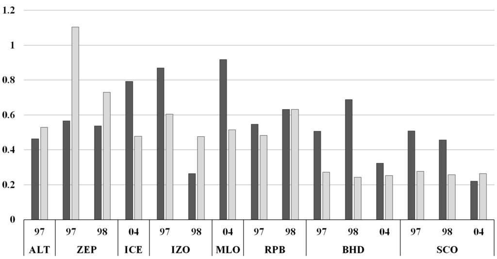
Figure 8. The ratio of a posteriori model-observation difference (simultaneous inversion) to a priori model-observation difference for concentration simulation (dark gray) and δ¹⁸O simulation (light gray).

These results indicate that each updated source contributed to improving both the modeled CO and δ¹⁸O while there was relatively small adjustment of the total CO inventory (Table 4). Thus, this suggests that an accurate estimation of source strength distribution is more important than the optimization of total CO emission in CO inversion analyses. Due to the advantages of including isotope information to the inversion analysis, more realistic source distributions were derived which sufficiently satisfy both measured CO and δ¹⁸O. Moreover, the improved δ¹⁸O fits provide additional confidence to the results that are obtained from CO-only inversions.

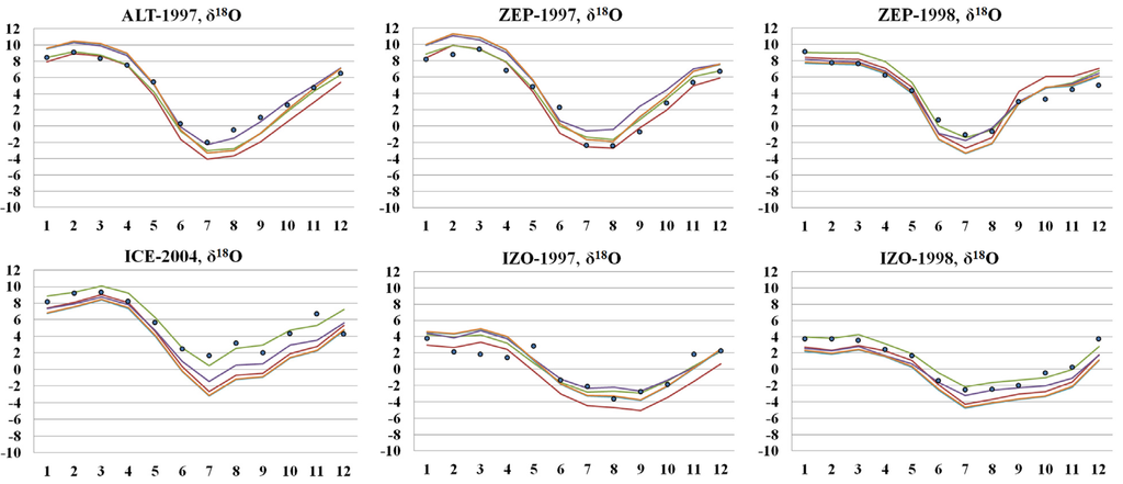
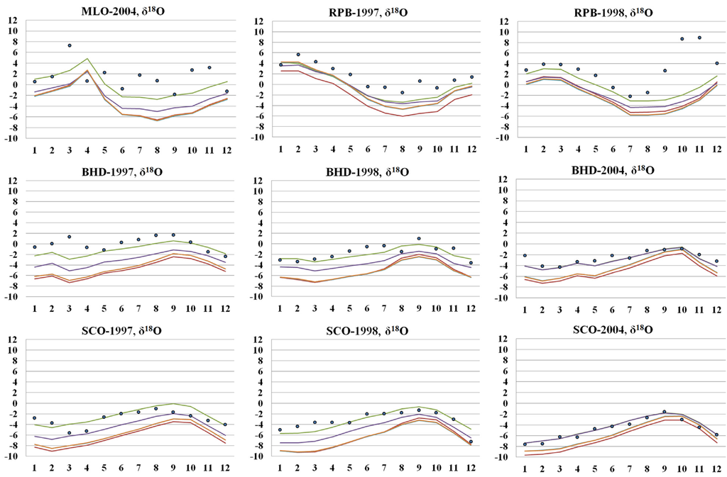
Figure 9. Comparison of a priori (brown line) and a posteriori modeled surface δ¹⁸O with measurements (blue dots). Green and purple lines denote a posteriori δ¹⁸O from simultaneous inversion and sequential inversion, respectively. Orange line is a posteriori δ¹⁸O with fixed isotope source signature. A posteriori isotope source signatures obtained from the simultaneous inversion are presented in the Table S7.

Figure 9. Comparison of a priori (brown line) and a posteriori modeled surface δ¹⁸O with measurements (blue dots). Green and purple lines denote a posteriori δ¹⁸O from simultaneous inversion and sequential inversion, respectively. Orange line is a posteriori δ¹⁸O with fixed isotope source signature. A posteriori isotope source signatures obtained from the simultaneous inversion are presented in the Table S7.

5.3. Inversion Results by Different Inversion Schemes: CO-only, Sequential, and Simultaneous Inversion

Various inversion schemes are tested and discussed in this section to elucidate the influence of different isotope information combining methods on the a posteriori source strength estimates.

Joint application of isotope ratio and concentration measurements generally gives more robust inversion results since the isotope ratios provide additional constraint. In Figure 10, a posteriori uncertainties of the three different inversion methods are presented. The sequential inversion provided the smallest uncertainties and always the biggest uncertainty was found in the CO-only inversion. The impact of different inversion methods on biomass burning, NMHC oxidation and the NH biofuel source is larger than that on other sources. Due to the small concentration of the minor source, biogenic and ocean sources are loosely constrained. The smaller a priori source uncertainties of fossil fuel and methane oxidation limit the influence of each inversion method. In the sequential inversion, the inverted data sets and the obtained uncertainties from the first inversion step are used as initial values for the second inversion (Equation (10)). The final uncertainties (error covariance, Ŝ; Equation (6)) of each source strength from the sequential inversion is obtained from the intermediate a posteriori source uncertainty term which is already once reduced using C¹⁶O information while the joint simultaneous inversion constrains the source only once.

Figure 10. Comparison of a posteriori uncertainty of three different inversion schemes: CO-only, sequential and simultaneous inversion.

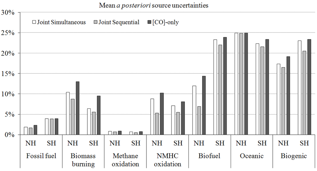
Figure 10. Comparison of a posteriori uncertainty of three different inversion schemes: CO-only, sequential and simultaneous inversion.

A basic underlying assumption of the Bayesian synthesis inversion is the linear relation between the source strengths and measurements. If the relation is nonlinear, as applies in the case of δ¹⁸O, the inversion should be iterated until converging. The linearity can be verified by comparing the results of the sequential and simultaneous inversions. If the results are different, this implies at least one of the measurement data sets is not linear with source change. Since the a posteriori source strengths from the two different methods are very similar in this study (approximately ±2% on average; Table 5), [C¹⁶O] and [C¹⁸O] appear to be linearly related to a change in source strength.

While the sequential and simultaneous inversions clearly improve the modeled δ¹⁸O and estimate similar a posteriori source strengths, the simultaneous inversion shows a significantly better fit to the observed δ¹⁸O (Figure 9). The averaged differences from the observation were derived to be 1.3‰ and 1.9‰ for the simultaneous inversion and sequential inversion, respectively.

In summary, insignificant a posteriori source inventory differences, especially between the joint sequential and joint simultaneous inversions, were found in the results of the three inversion schemes: CO-only, sequential and simultaneous inversions (Table 5). However, when [CO] and δ¹⁸O are jointly used in the inversion analyses, the optimized source strengths and δ¹⁸O were more reliable than the CO-only inversion results. The sequential use of the concentration and isotope information tends to reduce the a posteriori uncertainties more effectively (precision) and the simultaneous use of them shows smaller model-observation differences (accuracy).

5.4. The Influence of the Number of Observation Stations in the Inversion Results

In order to see the influence of the number of observation stations and the consistency of the inversion results with using different observational data sets, the sources of NH CO are constrained with 11 NOAA GMD surface station measurements (CO_NOAA).

Table 5. The ratios of optimization factors. seq/sim is ratio of optimization factor of sequential inversion to that of simultaneous inversion and CO/sim is ratio of optimization factor of CO-only inversion to that of simultaneous inversion. Mean deviation from the unity (identical result) is ±1.7% for seq/sim and ±4.6% for CO/sim.

		Fossil Fuel	Bio. Burn.	CH4 Ox.	NMHC Ox.	Biofuel	Oceanic	Biogenic
1997NH	seq/sim	0.99	0.98	0.99	0.98	1.04	0.99	1.00
	[CO]/sim	1.01	0.99	0.96	1.14	0.92	0.98	1.17
1998NH	seq/sim	1.00	1.00	1.00	0.97	1.03	1.00	1.00
	[CO]/sim	1.05	1.07	0.97	0.97	0.91	0.98	1.15
2004NH	seq/sim	1.00	1.00	1.00	0.94	1.00	0.99	1.18
	[CO]/sim	1.05	1.06	0.96	0.96	0.94	1.00	1.38
1997SH	seq/sim	1.00	0.99	0.99	0.98	1.00	0.99	1.00
	[CO]/sim	1.01	0.97	1.00	0.99	1.04	1.00	1.07
1998SH	seq/sim	1.00	1.01	1.00	0.97	0.99	0.99	0.99
	[CO]/sim	1.00	1.04	1.00	0.98	0.98	1.00	0.98
2004SH	seq/sim	0.99	0.98	0.99	1.02	0.98	0.98	0.97
	[CO]/sim	1.00	0.98	0.99	1.05	0.99	0.98	1.03

Table 5. The ratios of optimization factors. seq/sim is ratio of optimization factor of sequential inversion to that of simultaneous inversion and CO/sim is ratio of optimization factor of CO-only inversion to that of simultaneous inversion. Mean deviation from the unity (identical result) is ±1.7% for seq/sim and ±4.6% for CO/sim.

		Fossil Fuel	Bio. Burn.	CH4 Ox.	NMHC Ox.	Biofuel	Oceanic	Biogenic
1997NH	seq/sim	0.99	0.98	0.99	0.98	1.04	0.99	1.00
	[CO]/sim	1.01	0.99	0.96	1.14	0.92	0.98	1.17
1998NH	seq/sim	1.00	1.00	1.00	0.97	1.03	1.00	1.00
	[CO]/sim	1.05	1.07	0.97	0.97	0.91	0.98	1.15
2004NH	seq/sim	1.00	1.00	1.00	0.94	1.00	0.99	1.18
	[CO]/sim	1.05	1.06	0.96	0.96	0.94	1.00	1.38
1997SH	seq/sim	1.00	0.99	0.99	0.98	1.00	0.99	1.00
	[CO]/sim	1.01	0.97	1.00	0.99	1.04	1.00	1.07
1998SH	seq/sim	1.00	1.01	1.00	0.97	0.99	0.99	0.99
	[CO]/sim	1.00	1.04	1.00	0.98	0.98	1.00	0.98
2004SH	seq/sim	0.99	0.98	0.99	1.02	0.98	0.98	0.97
	[CO]/sim	1.00	0.98	0.99	1.05	0.99	0.98	1.03

CO_NOAA inversion results are very similar to the results of the joint inversion (Figure S5). For the biofuel and biogenic sources, although each method estimated notably different optimization factors, the discrepancies are within the uncertainty ranges. The difference between a posteriori concentrations of each inversion result and measured concentrations are compared in Figure 11. A similar degree of improvement from the a priori model-observation differences is found.

Figure 11. Comparison of model (a priori (orange) and a posteriori (green))—observation difference of the Northern Hemisphere.

Figure 11. Comparison of model (a priori (orange) and a posteriori (green))—observation difference of the Northern Hemisphere.

Therefore, consistency of a posteriori source strengths and model-observation differences between the CO_NOAA inversion and joint inversion results indicate that inversion results are sufficiently constrained despite the limited number of observations.

6. Summary and Conclusions

The simulation results from the tracer version of MOZART-4 reproduced observations of CO and δ¹⁸O fairly well in both hemispheres. The modeled and measured concentration showed a strong correlation (ρ = 0.94) and a small averaged model-observation difference (10.5 ppbv). In general, the model underestimated the concentration measurements in the NH and overestimated them in the SH. For δ¹⁸O, the correlation between the model and observation was 0.86 and the mean model-observation difference was 3‰. The model accurately reproduced observed δ¹⁸O at high latitude stations while modeled δ¹⁸O was lighter than observations at mid- and low latitude stations.

The joint inversion of CO and δ¹⁸O estimated total global CO production at 2951 TgCO/yr, 3084 TgCO/yr and 2583 TgCO/yr for 1997, 1998, and 2004 respectively. The a posteriori fossil fuel combustion source changed less than 5% in the SH and adjusted ±15% in the NH. The inversion result showed that the a priori biofuel inventory is significantly underestimated in the NH (up to 80%). For the biomass burning source, the a posteriori source did not change much. However, in 1997, the inversion analysis increased 33% compared to the a priori biomass burning source in the NH. The inversion result indicated a significant current overestimation of direct biogenic emission source (up to 50% in the NH). The methane oxidation source is considered to be a well-known source and its a posteriori source strength is similar to the a priori source strength. However, in the NH, ~10% more methane-derived CO was estimated, whereas ~3% less methane-derived CO was estimated in the SH.

The updated CO budget has improved agreement between data and model estimates of CO and δ¹⁸O, and this is seen more clearly in the oxygen isotope ratio, which can distinguish between different sources and so provide more accurate a posteriori source estimates. Moreover, this indicates the correct estimation of CO source distribution that can be obtained when isotope information is combined with concentration.

The joint inversion result was compared to the inversion result using CO measured from 11 NOAA GMD stations in the NH. While the two observational data sets are independent, the inversion results estimate similar a posteriori source strengths and interannual trends. Thus, the joint inversion reliably constrains the CO sources albeit a small number of observational stations. Also, CO concentration and δ¹⁸O were simultaneously and sequentially applied in the inversion analysis to find a more effective way for combining the two observations. While the sequential inversion provided more precise results (smaller a posteriori uncertainties), the simultaneous inversion more accurately constrained the CO sources, resulting in smaller model-observation differences.

References

- Brenninkmeijer, C.A.M.; Röckmann, T.; Bräunlich, M.; Jöckel, P.; Bergamaschi, P. Review of progress in isotope studies of atmospheric carbon monoxide. Chemosphere Glob. Chang. Sci. 1999, 1, 33–52. [Google Scholar] [CrossRef]
- Ehhalt, D.; Prather, M.; Dentener, F.; Derwent, R.; Dlugokencky, E.; Holland, E.; Isaksen, I.; Katima, J.; Kirchhoff, V.; Matson, P.; et al. Climate chamge 2001: The scientific basis (atmospheric chemistry and greenhouse gases). In Intergovernmental Panel on Climate Change Third Assessment Report; Cambridge University Press: Cambridge, UK, 2001. [Google Scholar]
- Crutzen, P.J.; Zimmermann, P.H. The changing photochemistry of the troposphere. Tellus Ser. A Dyn. Meteorol. Oceanogr. 1991, 43, 136–151. [Google Scholar] [CrossRef]
- Thompson, A.M. The oxidizing capacity of the earth’s atmosphere: Probable past and future changes. Science 1992, 256, 1157–1165. [Google Scholar] [CrossRef] [PubMed]
- Forster, P.; Ramaswamy, V.; Artaxo, P.; Berntsen, T.; Betts, R.; Fahey, D.; Haywood, J.; Lean, J.; Lowe, D.; Myhre, G.; et al. Changes in atmospheric constituents and in radiative forcing. In Climate Change 2007: The Physical Science Basis: Contribution of Working Group i to the Fourth Assessment Report of the Intergovernmental Panel on Climate Change; Solomon, S., Qin, D., Manning, M., Chen, Z., Marquis, M., Averyt, K., Tignor, M., Miller, H., Eds.; Cambridge University Press: Cambridge, UK, 2007; pp. 129–234. [Google Scholar]
- Li, Q.; Jacob, D.J.; Bey, I.; Palmer, P.I.; Duncan, B.N.; Field, B.D.; Martin, R.V.; Fiore, A.M.; Yantosca, R.M.; Parrish, D.D.; et al. Transatlantic transport of pollution and its effects on surface ozone in Europe and North America. J. Geophys. Res. 2002, 107. [Google Scholar] [CrossRef]
- Shim, C.; Li, Q.; Luo, M.; Kulawik, S.; Worden, H.; Worden, J.; Eldering, A.; Diskin, G.; Sachse, G.; Weinheimer, A.; et al. Satellite observations of mexico city pollution outflow from the Tropospheric Emissions Spectrometer (TES). Atmos. Environ. 2009, 43, 1540–1547. [Google Scholar] [CrossRef]
- Pfister, G.; Hess, P.G.; Emmons, L.K.; Lamarque, J.F.; Wiedinmyer, C.; Edwards, D.P.; Pétron, G.; Gille, J.C.; Sachse, G.W. Quantifying CO emissions from the 2004 alaskan wildfires using mopitt co data. Geophys. Res. Lett. 2005, 32, L11809. [Google Scholar] [CrossRef]
- Palmer, P.I.; Suntharalingam, P.; Jones, D.B.A.; Jacob, D.J.; Streets, D.G.; Fu, Q.; Vay, S.A.; Sachse, G.W. Using CO2: CO correlations to improve inverse analyses of carbon fluxes. J. Geophys. Res. 2006, 111, D12318. [Google Scholar] [CrossRef]
- Brenninkmeijer, C.A.M.; Rockmann, T. Principal factors determining the 18O/16O ratio of atmospheric CO as derived from observations in the southern hemispheric troposphere and lowermost stratosphere. J. Geophys. Res. Atmos. 1997, 102, 25477–25485. [Google Scholar] [CrossRef]
- Hauglustaine, D.A.; Brasseur, G.P.; Walters, S.; Rasch, P.J.; Muller, J.F.; Emmons, L.K.; Carroll, C.A. Mozart, a global chemical transport model for ozone and related chemical tracers 2. Model results and evaluation. J. Geophys. Res. Atmos. 1998, 103, 28291–28335. [Google Scholar] [CrossRef]
- Logan, J.A.; Prather, M.J.; Wofsy, S.C.; McElroy, M.B. Tropospheric chemistry: A global perspective. J. Geophys. Res. Oceans Atmos. 1981, 86, 7210–7254. [Google Scholar] [CrossRef]
- Weinstock, B.; Niki, H. Carbon monoxide balance in nature. Science 1972, 176, 290–292. [Google Scholar] [CrossRef] [PubMed]
- Bergamaschi, P.; Hein, R.; Heimann, M.; Crutzen, P.J. Inverse modeling of the global CO cycle 1. Inversion of CO mixing ratios. J. Geophys. Res. 2000, 105, 1909–1927. [Google Scholar] [CrossRef]
- Sanhueza, E.; Dong, Y.; Scharffe, D.; Lobert, J.M.; Crutzen, P.J. Carbon monoxide uptake by temperate forest soils: The effects of leaves and humus layers. Tellus Ser. B Chem. Phys. Meteorol. 1998, 50, 51–58. [Google Scholar] [CrossRef]
- Pétron, G.; Granier, C.; Khattatov, B.; Lamarque, J.-F.; Yudin, V.; Müller, J.-F.; Gille, J. Inverse modeling of carbon monoxide surface emissions using climate monitoring and diagnostics laboratory network observations. J. Geophys. Res. 2002, 107, 4761. [Google Scholar] [CrossRef]
- Pétron, G.; Granier, C.; Khattatov, B.; Yudin, V.; Lamarque, J.-F.; Emmons, L.; Gille, J.; Edwards, D.P. Monthly CO surface sources inventory based on the 2000–2001 mopitt satellite data. Geophys. Res. Lett. 2004, 31, L21107. [Google Scholar] [CrossRef]
- Müller, J.F.; Stavrakou, T. Inversion of CO and nox emissions using the adjoint of the images model. Atmos. Chem. Phys. 2005, 5, 1157–1186. [Google Scholar] [CrossRef]
- Kasibhatla, P.; Arellano, A.; Logan, J.A.; Palmer, P.I.; Novelli, P. Top-down estimate of a large source of atmospheric carbon monoxide associated with fuel combustion in asia. Geophys. Res. Lett. 2002, 29. [Google Scholar] [CrossRef]
- Arellano, A.F., Jr.; Kasibhatla, P.S.; Giglio, L.; van der Werf, G.R.; Randerson, J.T. Top-down estimates of global CO sources using mopitt measurements. Geophys. Res. Lett. 2004, 31, L01104. [Google Scholar]
- Arellano, A.F., Jr.; Kasibhatla, P.S.; Giglio, L.; van der Werf, G.R.; Randerson, J.T.; Collatz, G.J. Time-dependent inversion estimates of global biomass-burning CO emissions using measurement of pollution in the troposphere (mopitt) measurements. J. Geophys. Res. 2006, 111, D09303. [Google Scholar]
- Hooghiemstra, P.B.; Krol, M.C.; Bergamaschi, P.; de Laat, A.T.J.; van der Werf, G.R.; Novelli, P.C.; Deeter, M.N.; Aben, I.; Röckmann, T. Comparing optimized CO emission estimates using mopitt or noaa surface network observations. J. Geophys. Res. Atmos. 2012, 117, D06309. [Google Scholar]
- Kopacz, M.; Jacob, D.J.; Fisher, J.A.; Logan, J.A.; Zhang, L.; Megretskaia, I.A.; Yantosca, R.M.; Singh, K.; Henze, D.K.; Burrows, J.P.; et al. Global estimates of CO sources with high resolution by adjoint inversion of multiple satellite datasets (mopitt, airs, sciamachy, tes). Atmos. Chem. Phys. 2010, 10, 855–876. [Google Scholar] [CrossRef]
- Bergamaschi, P.; Hein, R.; Brenninkmeijer, C.A.M.; Crutzen, P.J. Inverse modeling of the global CO cycle 2. Inversion of 13c/12c and 18o/16o isotope ratios. J. Geophys. Res. 2000, 105, 1929–1945. [Google Scholar] [CrossRef]
- Tans, P.P. A note on isotopic ratios and the global atmospheric methane budget. Glob. Biogeochem. Cycles 1997, 11, 77–81. [Google Scholar] [CrossRef]
- Rayner, P.J.; Law, R.M.; Allison, C.E.; Francey, R.J.; Trudinger, C.M.; Pickett-Heaps, C. Interannual variability of the global carbon cycle (1992–2005) inferred by inversion of atmospheric CO2 and δ13CO2 measurements. Glob. Biogeochem. Cycles 2008, 22, GB3008. [Google Scholar] [CrossRef]
- Rockmann, T.; Jockel, P.; Gros, V.; Braunlich, M.; Possnert, G.; Brenninkmeijer, C.A.M. Using 14C, 13C, 18O and 17O isotopic variations to provide insights into the high northern latitude surface CO inventory. Atmos. Chem. Phys. 2002, 2, 147–159. [Google Scholar] [CrossRef]
- Enting, I.G. Inverse Problems in Atmospheric Constituent Transport; Cambridge University Press: Cambridge, UK, 2002. [Google Scholar]
- Tans, P.P.; Berry, J.A.; Keeling, R.F. Oceanic C-13/C-12 observations—A new window on ocean CO2 uptake. Glob. Biogeochem. Cycles 1993, 7, 353–368. [Google Scholar] [CrossRef]
- Mikaloff Fletcher, S.E.; Tans, P.P.; Bruhwiler, L.M.; Miller, J.B.; Heimann, M. CH4 sources estimated from atmospheric observations of CH4 and its 13C/12C isotopic ratios: 1. Inverse modeling of source processes. Glob. Biogeochem. Cycles 2004, 18, GB4004. [Google Scholar]
- Ciais, P.; Tans, P.P.; White, J. W. C.; Trolier, M.; Francey, R.J.; Berry, J. A.; Randall, D.R.; Sellers, P.J.; Collatz, J.G.; Schimel, D.S. Partitioning of ocean and land uptake of CO2 as inferred by delta13C measurements from the noaa climate monitoring and diagnostics laboratory global air sampling network. J. Geophys. Res. Atmos. 1995, 100, 5051–5070. [Google Scholar] [CrossRef]
- Houweling, S.; van der Werf, G.R.; Klein Goldewijk, K.; Röckmann, T.; Aben, I. Early anthropogenic CH4 emissions and the variation of CH4 and 13CH4 over the last millennium. Glob. Biogeochem. Cycles 2008, 22, GB1002. [Google Scholar] [CrossRef]
- Hein, R.; Crutzen, P.J.; Heimann, M. An inverse modeling approach to investigate the global atmospheric methane cycle. Glob. Biogeochem. Cycles 1997, 11, 43–76. [Google Scholar] [CrossRef]
- Emmons, L.K.; Walters, S.; Hess, P.G.; Lamarque, J.F.; Pfister, G.G.; Fillmore, D.; Granier, C.; Guenther, A.; Kinnison, D.; Laepple, T.; et al. Description and evaluation of the model for ozone and related chemical tracers, version 4 (mozart-4). Geosci. Model Dev. 2010, 3, 43–67. [Google Scholar] [CrossRef]
- Manning, M.R.; Brenninkmeijer, C.A.M.; Allan, W. Atmospheric carbon monoxide budget of the southern hemisphere: Implications of 13c/12c measurements. J. Geophys. Res. 1997, 102, 10673–10682. [Google Scholar] [CrossRef]
- Mak, J.E.; Kra, G.; Sandomenico, T.; Bergamaschi, P. The seasonally varying isotopic composition of the sources of carbon monoxide at barbados, west indies. J. Geophys. Res. 2003, 108. [Google Scholar] [CrossRef]
- Novelli, P.C.; Masarie, K.A.; Lang, P.M.; Hall, B.D.; Myers, R.C.; Elkins, J.W. Reanalysis of tropospheric CO trends: Effects of the 1997–1998 wildfires. J. Geophys. Res. 2003, 108. [Google Scholar] [CrossRef]
- Novelli, P.C.; Masarie, K.A.; Lang, P.M. Distributions and recent changes of carbon monoxide in the lower troposphere. J. Geophys. Res. 1998, 103, 19015–19033. [Google Scholar] [CrossRef]
- Pfister, G.G.; Emmons, L.K.; Hess, P.G.; Lamarque, J.F.; Orlando, J.J.; Walters, S.; Guenther, A.; Palmer, P.I.; Lawrence, P.J. Contribution of isoprene to chemical budgets: A model tracer study with the ncar ctm mozart-4. J. Geophys. Res. 2008, 113, D05308. [Google Scholar]
- Williams, J.; Fischer, H.; Wong, S.; Crutzen, P.J.; Scheele, M.P.; Lelieveld, J. Near equatorial CO and O3 profiles over the indian ocean during the winter monsoon: High O3 levels in the middle troposphere and interhemispheric exchange. J. Geophys. Res. 2002, 107. [Google Scholar] [CrossRef]
- Mak, J.E.; Brenninkmeijer, C.A.M. Compressed air sample technology for the isotopic analysis of atmospheric carbon monoxide. J. Atmos. Ocean. Technol. 1994, 11, 425–431. [Google Scholar]
- Brenninkmeijer, C.A.M. Measurement of the abundance of 14CO in the atmosphere and the 13C/12C and 18O/16O ration of atmospheric co with applications in new zealand and antarctica. J. Geophys. Res. 1993, 98, 10595–10614. [Google Scholar] [CrossRef]
- Mak, J.; Kra, G. The isotopic composition of carbon monoxide at montauk point, long island. Chemosphere Glob. Chang. Sci. 1999, 1, 205–218. [Google Scholar] [CrossRef]
- Smiley, W.G. Note on a reagent for oxidation of carbon monoxide. Nucl. Sci. Abstr. 1965, 3, 391. [Google Scholar]
- Drori, R.; Dayan, U.; Edwards, D.P.; Emmons, L.K.; Erlick, C. Attributing and quantifying carbon monoxide sources affecting the eastern mediterranean: A combined satellite, modelling, and synoptic analysis study. Atmos. Chem. Phys. 2012, 12, 1067–1082. [Google Scholar] [CrossRef]
- Emmons, L.K.; Apel, E.C.; Lamarque, J.F.; Hess, P.G.; Avery, M.; Blake, D.; Brune, W.; Campos, T.; Crawford, J.; DeCarlo, P.F.; et al. Impact of mexico city emissions on regional air quality from mozart-4 simulations. Atmos. Chem. Phys. 2010, 10, 6195–6212. [Google Scholar] [CrossRef]
- Wespes, C.; Emmons, L.; Edwards, D.P.; Hannigan, J.; Hurtmans, D.; Saunois, M.; Coheur, P.F.; Clerbaux, C.; Coffey, M.T.; Batchelor, R.L.; et al. Analysis of ozone and nitric acid in spring and summer arctic pollution using aircraft, ground-based, satellite observations and mozart-4 model: Source attribution and partitioning. Atmos. Chem. Phys. 2012, 12, 237–259. [Google Scholar] [CrossRef]
- Pfister, G.G.; Hess, P.G.; Emmons, L.K.; Rasch, P.J.; Vitt, F.M. Impact of the summer 2004 alaska fires on top of the atmosphere clear-sky radiation fluxes. J. Geophys. Res. 2008, 113, D02204. [Google Scholar]
- Shindell, D.T.; Faluvegi, G.; Stevenson, D.S.; Krol, M.C.; Emmons, L.K.; Lamarque, J.F.; Pétron, G.; Dentener, F.J.; Ellingsen, K.; Schultz, M.G.; et al. Multimodel simulations of carbon monoxide: Comparison with observations and projected near-future changes. J. Geophys. Res. 2006, 111, D19306. [Google Scholar] [CrossRef]
- Stevenson, D.S.; Dentener, F.J.; Schultz, M.G.; Ellingsen, K.; van Noije, T.P.C.; Wild, O.; Zeng, G.; Amann, M.; Atherton, C.S.; Bell, N.; et al. Multimodel ensemble simulations of present-day and near-future tropospheric ozone. J. Geophys. Res. 2006, 111, D08301. [Google Scholar]
- Emmons, L.K.; Hess, P.G.; Lamarque, J.F.; Pfister, G.G. Tagged ozone mechanism for mozart-4, cam-chem and other chemical transport models. Geosci. Model Dev. 2012, 5, 1531–1542. [Google Scholar] [CrossRef]
- Kalnay, E.; Kanamitsu, M.; Kistler, R.; Collins, W.; Deaven, D.; Gandin, L.; Iredell, M.; Saha, S.; White, G.; Woollen, J.; et al. The ncep/ncar 40-year reanalysis project. Bull. Am. Meteorol. Soc. 1996, 77, 437–471. [Google Scholar]
- Kistler, R.; Collins, W.; Saha, S.; White, G.; Woollen, J.; Kalnay, E.; Chelliah, M.; Ebisuzaki, W.; Kanamitsu, M.; Kousky, V.; et al. The NCEP–NCAR 50–year reanalysis: Monthly means CD–ROM and documentation. Bull. Am. Meteorol. Soc. 2001, 82, 247–267. [Google Scholar]
- Van der Werf, G.R.; Randerson, J.T.; Giglio, L.; Collatz, G.J.; Kasibhatla, P.S.; Arellano, A.F. Interannual variability in global biomass burning emissions from 1997 to 2004. Atmos. Chem. Phys. 2006, 6, 3423–3441. [Google Scholar] [CrossRef]
- Tarr, M.A.; Miller, W.L.; Zepp, R.G. Direct carbon monoxide photoproduction from plant matter. J. Geophys. Res. Atmos. 1995, 100, 11403–11413. [Google Scholar] [CrossRef]
- Conrad, R.; Seiler, W.; Bunse, G.; Giehl, H. Carbon monoxide in seawater (Atlantic Ocean). J. Geophys. Res. 1982, 87, 8839–8852. [Google Scholar] [CrossRef]
- Stubbins, A.; Uher, G.; Kitidis, V.; Law, C.S.; Upstill-Goddard, R.C.; Woodward, E.M.S. The open-ocean source of atmospheric carbon monoxide. Deep Sea Res. Part II Top. Stud. Oceanogr. 2006, 53, 1685–1694. [Google Scholar] [CrossRef]
- Olivier, J.; Peters, J.; Granier, C.; Petron, G.; Müller, J.F.; Wallens, S. Present and future surface emissions of atmospheric compounds. POET report #2. 2003. EU project EVK2–1999–00011 Available online: http://tropo.aeronomie.be/pdf/POET_emissions_report.pdf (accessed on 17 April 2015).
- Horowitz, L.W.; Walters, S.; Mauzerall, D.L.; Emmons, L.K.; Rasch, P.J.; Granier, C.; Tie, X.; Lamarque, J.-F.; Schultz, M.G.; Tyndall, G.S.; et al. A global simulation of tropospheric ozone and related tracers: Description and evaluation of mozart, version 2. J. Geophys. Res. 2003, 108. [Google Scholar] [CrossRef]
- Lawrence, M.G.; Jöckel, P.; von Kuhlmann, R. What does the global mean OH concentration tell us? Atmos. Chem. Phys. 2001, 1, 37–49. [Google Scholar] [CrossRef]
- Sanderson, M.G.; Collins, W.J.; Derwent, R.G.; Johnson, C.E. Simulation of global hydrogen levels using a lagrangian three-dimensional model. J. Atmos. Chem. 2003, 46, 15–28. [Google Scholar] [CrossRef]
- Stevens, C.M.; Wagner, A.F. The role of isotope fractionation effects in atmospheric chemistry. Z. Naturforschung 1989, 44, 376–384. [Google Scholar]
- Röckmann, T.; Brenninkmeijer, C.A.M.; Saueressig, G.; Bergamaschi, P.; Crowley, J.N.; Fischer, H.; Crutzen, P.J. Mass-independent oxygen isotope fractionation in atmospheric CO as a result of the reaction CO + OH. Science 1998, 281, 544–546. [Google Scholar] [CrossRef] [PubMed]
- Tsunogai, U.; Nakagawa, F.; Komatsu, D.D.; Gamo, T. Stable carbon and oxygen isotopic analysis of atmospheric carbon monoxide using continuous-flow isotope ratio ms by isotope ratio monitoring of CO. Anal. Chem. 2002, 74, 5695–5700. [Google Scholar] [CrossRef] [PubMed]
- Stevens, C.M.; Walling, D.; Venters, A.; Ross, L.E.; Engelkem, A.; Krout, L. Isotopic composition of atmospheric carbon-monoxide. Earth Planet. Sci. Lett. 1972, 16, 147–165. [Google Scholar] [CrossRef]
- Nakagawa, F.; Tsunogai, U.; Gamo, T.; Yoshida, N. Stable isotopic compositions and fractionations of carbon monoxide at coastal and open ocean stations in the Pacific. J. Geophys. Res. Oceans 2004, 109. [Google Scholar] [CrossRef]
- Guenther, A.; Geron, C.; Pierce, T.; Lamb, B.; Harley, P.; Fall, R. Natural emissions of non-methane volatile organic compounds; carbon monoxide, and oxides of nitrogen from North America. Atmos. Environ. 2000, 34, 2205–2230. [Google Scholar] [CrossRef]
- Duncan, B.N.; Logan, J.A.; Bey, I.; Megretskaia, I.A.; Yantosca, R.M.; Novelli, P.C.; Jones, N.B.; Rinsland, C.P. Global budget of co, 1988–997: Source estimates and validation with a global model. J. Geophys. Res. 2007, 112, D22301. [Google Scholar] [CrossRef]
- Palmer, P.I.; Jacob, D.J.; Jones, D.B.A.; Heald, C.L.; Yantosca, R.M.; Logan, J.A.; Sachse, G.W.; Streets, D.G. Inverting for emissions of carbon monoxide from asia using aircraft observations over the western pacific. J. Geophys. Res. 2003, 108. [Google Scholar] [CrossRef]
- Bousquet, P.; Ciais, P.; Peylin, P.; Ramonet, M.; Monfray, P. Inverse modeling of annual atmospheric CO2 sources and sinks 1. Method and control inversion. J. Geophys. Res. 1999, 104, 26161–26178. [Google Scholar] [CrossRef]
- Bousquet, P.; Peylin, P.; Ciais, P.; Ramonet, M.; Monfray, P. Inverse modeling of annual atmospheric CO2 sources and sinks 2. Sensitivity study. J. Geophys. Res. 1999, 104, 26179–26193. [Google Scholar] [CrossRef]
- Chen, Y.-H.; Prinn, R.G. Estimation of atmospheric methane emissions between 1996 and 2001 using a three-dimensional global chemical transport model. J. Geophys. Res. 2006, 111, D10307. [Google Scholar] [CrossRef]
- Heimann, M.; Kaminski, T. Inverse modelling approaches to infer surface trace gas fluxes from observed atmospheric mixing ratios. In Developments in Atmospheric Science; Bouwman, A.F., Ed.; Elsevier: Amsterdam, Netherlands, 1999; Volume 24, pp. 277–295. [Google Scholar]
- Bian, H.; Chin, M.; Kawa, S.R.; Duncan, B.; Arellano, A.; Kasibhatla, P. Sensitivity of global co simulations to uncertainties in biomass burning sources. J. Geophys. Res. 2007, 112, D23308. [Google Scholar] [CrossRef]
- Heald, C.L.; Jacob, D.J.; Jones, D.B.A.; Palmer, P.I.; Logan, J.A.; Streets, D.G.; Sachse, G.W.; Gille, J.C.; Hoffman, R.N.; Nehrkorn, T. Comparative inverse analysis of satellite (mopitt) and aircraft (trace-p) observations to estimate asian sources of carbon monoxide. J. Geophys. Res. 2004, 109, D23306. [Google Scholar]
- Dentener, F.; Peters, W.; Krol, M.; van Weele, M.; Bergamaschi, P.; Lelieveld, J. Interannual variability and trend of ch4 lifetime as a measure for OH changes in the 1979–1993 time period. J. Geophys. Res. 2003, 108. [Google Scholar] [CrossRef]
- Pilkington, M. Joint inversion of gravity and magnetic data for two-layer models. Geophysics 2006, 71, 35–42. [Google Scholar] [CrossRef]
- Miller, J.B.; Mack, K.A.; Dissly, R.; White, J.W.C.; Dlugokencky, E.J.; Tans, P.P. Development of analytical methods and measurements of 13C/12C in atmospheric ch4 from the NOAA climate monitoring and diagnostics laboratory global air sampling network. J. Geophys. Res. 2002, 107, 4178. [Google Scholar] [CrossRef]
- GLOBALVIEW-CH4. Cooperative atmospheric data integration project—Methane. CD-ROM, NOAA ESRL, Boulder, Colorado. Available online: ftp.Cmdl.Noaa.Gov, path: Ccg/ch4/globalview (accessed on 17 April 2015).
- Lines, L.R.; Schultz, A.K.; Treitel, S. Cooperative inversion of geophysical data. Geophysics 1988, 53, 8–20. [Google Scholar] [CrossRef]
- Tsunogai, U.; Hachisu, Y.; Komatsu, D.D.; Nakagawa, F.; Gamo, T.; Akiyama, K.-I. An updated estimation of the stable carbon and oxygen isotopic compositions of automobile CO emissions. Atmos. Environ. 2003, 37, 4901–4910. [Google Scholar] [CrossRef]
- Bergamaschi, P.; Brenninkmeijer, C.A.M.; Hahn, M.; Rockmann, T.; Scharffe, D.H.; Crutzen, P.J.; Elansky, N.F.; Belikov, I.B.; Trivett, N.B.A.; Worthy, D.E.J. Isotope analysis based source identification for atmospheric CH4 and CO sampled across russia using the trans-siberian railroad. J. Geophys. Res. Atmos. 1998, 103, 8227–8235. [Google Scholar] [CrossRef]
- Kato, S.; Akimoto, H.; Röckmann, T.; Bräunlich, M.; Brenninkmeijer, C.A.M. Stable isotopic compositions of carbon monoxide from biomass burning experiments. Atmos. Environ. 1999, 33, 4357–4362. [Google Scholar]
- Park, K.; Emmons, L.K.; Wang, Z.; Mak, J.E. Large interannual variations in nonmethane volatile organic compound emissions based on measurements of carbon monoxide. Geophys. Res. Lett. 2013, 40, 221–226. [Google Scholar] [CrossRef]
- Conny, J.M.; Verkouteren, R.M.; Currie, L.A. Carbon 13 composition of tropospheric CO in Brazil: A model scenario during the biomass burn season. J. Geophys. Res. Atmos. 1997, 102, 10,638–10,693. [Google Scholar] [CrossRef]
- Conny, J.M. The isotopic characterization of carbon monoxide in the troposphere. Atmos. Environ. 1999, 32, 2669–2683. [Google Scholar] [CrossRef]
- Quay, P.D.; King, S.L.; Stutsman, J.; Wilbur, D.O.; Steele, L.P.; Fung, I.; Gammon, R.H.; Brown, T.A.; Farwell, G.W.; Grootes, P.M.; Schmidt, F.H. Carbon isotopic composition of atmospheric CH4: Fossil and biomass burning source strengths. Glob. Biogeochem. Cycles 1991, 5, 25–47. [Google Scholar] [CrossRef]
- Röckman, T.; Brenninkmeijer, C.A.M.; Crutzen, P.J.; Platt, U. Short term variations in the 13C/12C ratio of CO as a measure of Cl activation during tropospheric ozone depletion events in the Arctic. J. Geophys. Res. Atmos. 1999, 104, 1691–1697. [Google Scholar] [CrossRef]
- Moss, R.; Manning, M.; Lowe, D.; Ferretti, D.; Knobben, R. Changes in atmospheric carbon monoxide in the Pacific region. In Workshop on the Science of Atmospheric Trace Gases; NIWA: Wellington, New Zealand, 1998; Clarkson, T., Ed.; pp. 74–77. [Google Scholar]
© 2015 by the authors; licensee MDPI, Basel, Switzerland. This article is an open access article distributed under the terms and conditions of the Creative Commons Attribution license (http://creativecommons.org/licenses/by/4.0/).