Article

Evapotranspiration Estimates over Non-Homogeneous Mediterranean Land Cover by a Calibrated “Critical Resistance” Approach

CNR—Istituto di Scienze dell'Atmosfera e del Clima, U.O. S. Lecce, Via Monteroni, 73100 Lecce, Italy
Atmosphere 2015, 6(3), 255-272; https://doi.org/10.3390/atmos6030255
Submission received: 5 November 2014 / Revised: 16 January 2015 / Accepted: 29 January 2015 / Published: 27 February 2015

Abstract

:
An approach based on the Penman-Monteith equation was used to estimate the actual evapotranspiration from local meteorological data over non-homogeneous land cover in a Mediterranean site in the south-east of Italy, with two six month data sets from two different years of measurements (2006 and 2009). The “critical resistance” formulation was used in different forms to model the surface resistance, together with some modifications to take into account the soil moisture content. One, two, or three model parameters were estimated, one of them related to the atmospheric resistance and the others to the surface resistance, and the calibration was made by either linear regression or nonlinear minimization of a proper cost function, depending on the applicability. Two kinds of cost functions were tested, the first depending on both the latent heat flux and the difference between screen air temperature and surface radiometric temperature, and the second depending on the temperature difference only. In all cases the calculated fluxes give better results with respect to both a flux-gradient approach and a complementarity based method, that require comparable data inputs. However the calibration by the temperature differences only, that requires no turbulent flux measurements, considerably increases the statistical uncertainty of the calibration parameters. The inclusion of the soil moisture did not significantly improve the model results in the considered site.

1. Introduction

Evapotranspiration is a main component of surface energy, water budget, and of the water cycle, and is of great importance, from micrometeorological to climate and water availability projection studies. Thus improving evapotranspiration estimations and measurements from the local to the global scale is still a research challenge for the meteorological and hydrological scientific community [1].
The use of radiative energy input (either total or net radiation) together with surface radiometric temperature data (“brightness temperature”, [2]) as basic information for evapotranspiration and turbulent surface fluxes estimations has been studied for several years in different forms, generally in the context of fluxes recovered from satellite data [3].
Many different methods have been proposed, some of which are directly based on the correlation between the spatial variability of the surface temperature and the evaporation fluxes and need a large amount of area distributed data to span the maximum regional surface temperature interval for calibrating the 0–1 interval of evaporative fraction [4,5]. Other methods require just “local” input data, i.e., representative of the flux footprint source area, and parameter values equally related to the local surface characteristics. A complex description of the surface features is used in Land Surface Models (LSM) and Soil Vegetation Atmosphere Transfer models (SVAT), with the necessity of a large number of “effective” surface parameters not always easy to be calculated and/or calibrated [6,7]. It follows that more complex models are not always associated with better performances in flux estimations [3]. Here, attention is focused on simpler local data models with a small number of parameters, that are in general based either on vertical flux-gradient relations (e.g., SEBS, [8]) that can also distinguish between bare soil and canopy contributions [9], or thermodynamic algorithms often based on the complementarity principle [10,11]. Depending on the specific model, the surface temperature data need to be integrated by additional local meteorological information (air temperature/humidity, wind speed) and/or parameters containing basic surface information such as aerodynamic roughness and Leaf-Area Index (LAI). However, in methods involving flux-gradient approaches the evaluation of the surface roughness parameters can be misleading, as they are normally associated to the aerodynamic surface temperature that is often quite different (even several degrees) from the measured radiometric temperature [12]. These problems can be overcome in principle by a direct calibration of the surface resistance parameters with respect to the air-surface measured temperature differences and fluxes. In addition, direct calculations of heat fluxes from temperature gradients are restricted by the availability and the uncertainty of surface temperature measurements. Indeed the statistical error due to the uncertainty of the measured air-surface temperature difference can be of some tens in percent value, and can correspond to an error of the same amount or greater in the calculated fluxes [13]. In these cases the evaporation flux is generally obtained as residue of the surface energy balance, carrying even larger uncertainty. On the other hand, local data based methods for directly calculating the latent flux from Priestley-Taylor (PT) or Penman equations have also been proposed, often in association with the complementarity principle [10]. Venturini et al. [11] used the complementarity principle together with the PT equation and a thermodynamic calculation based on a two point interpolation of the water vapour saturation curve to obtain the surface water vapour pressure, estimating the evapotranspiration flux with no need of local parameter calibration in principle. However they did not exclude the possibility of a better local tuning of the interpolation procedure to ensure good applicability in different surface conditions.
The Penman-Monteith (PM) equation [14] has been widely used for evaluating reference evapotranspiration over homogeneous canopies (crops), where it has already been assumed as reference procedure to determine crop water requirements [15]. In the case of reference evapotranspiration the standardized characteristics of the surface (canopy height, LAI, and surface moisture) allow the use of parameters depending only on the crop type for both the surface resistance and the atmospheric resistance in the case of daily averaged evapotranspiration estimates, as discussed by Allen et al. [16]. In this scheme the parameter values for estimating evapotranspiration for different well watered crops have been tabulated and standardized for practical application in the calculation of the water requirements in different climate conditions [15]. The reference evapotranspiration from the PM equation has been also used to estimate the real evapotranspiration over cultivars and also natural vegetated areas by the use of correction coefficients based for example on satellite vegetation indexes [17,18]. However, even for the reference evapotranspiration, it was noted that different day/night values for the surface resistance have to be used to guarantee correct daily averages if the PM expression is applied for periods shorter than a diurnal cycle [16]. This shows a somehow expected dependence of the surface resistance response on the incident radiative fluxes.
An analysis of the surface “bulk” resistance R0 in the PM equation was performed by Alves and Pereira [19], together with an intercomparison with the functional forms of the multiplicative functions proposed by Jarvis [20] to model a canopy resistance. They showed that the PM equation requires a well-defined functional dependence of the surface resistance from the meteorological variables of the same equation (available energy flux, air humidity deficit, and temperature) and that these functional forms are in agreement with the semi-empirical expressions adopted by Jarvis [20] for available radiative flux and humidity deficit.
A dimensional analysis of the PM equation by Katerji and Perrier [21] had shown similar results for the functional form of the surface resistance, that appeared to be a function of a “critical resistance” R*, which can be considered the surface resistance value that decouples the canopy evapotranspiration from the atmospheric resistance effects; this with a form in agreement with the results found by Alves and Pereira [19].
Rana et al. [22] used the concept of critical resistance to model the actual evapotranspiration over crops. In this model the surface (crop) resistance depends linearly on the critical resistance but the linear coefficients are shown to depend on the crop moisture availability. They found the measured predawn leaf water potential of the crop to be a good parameter for describing how the canopy moisture availability affects the surface resistance and obtained a simple model for the actual evapotranspiration even in water stress conditions for homogeneous crops, where the predawn water potential can be determined by direct measurements. Rana et al. [23] also simplified this result proposing a “crop coefficient” model in which an empirical relation between the leaf water potential and the measured soil water moisture is used in the field. Katerji and Rana [24] also showed that the “critical resistance” approach to model a canopy resistance that varies with local meteorology gives better estimations of the actual evapotranspiration compared with a constant locally determined canopy resistance, especially for hourly scale measurements and tall crops, in different kinds of sites and cultivars.
The above mentioned studies show that the PM equation admits a dependence of the surface resistance on the local meteorological variables in the same equation (energy flux input, air humidity deficit, and temperature) and that its functional form is somehow independent of the surface characteristics but defined by similarity properties of the equation as function of a “critical resistance”. They also show that varying the functional coefficients with the water stress allows PM based models to be used for actual evapotranspiration estimates also in semi-arid climate conditions. These considerations about the prescribed functional form of the surface resistance in the PM equation also suggest the possibility of extending its application to natural canopies, in which however both the atmospheric resistance parameters and the surface resistance parameters can be difficult to be determined, either from the canopy characteristics or by direct measurements, and should be recovered by calibration procedures.
Stewart [25] applied the PM equation with the Jarvis [20] approach for the surface resistance to model the evapotranspiration of a pine forest, after experimentally calibrating several model parameters by a multivariate method. He obtained the best results with a surface resistance depending non-linearly on the local meteorology and the available soil moisture, for which an explained variance of the order of 70% was obtained. Shuttleworth and Wallace (SW) [26] proposed a model based on a development of the PM equation to take into account partially shaded canopy surfaces (sparse crops). It separates the radiation and evapotranspiration contributions from the canopy and the partially shaded underlying surface using a LAI-based parameterization. Stannard [27] compared the results of the SW model with measurements in a semiarid region and with the results of the PT and PM model, again using the Jarvis [20] formulation for the canopy resistance. He found that the SW model, that separates the soil from the canopy evaporative contributions, performs better that the PM big-leaf model with a single surface resistance in the site, characterized by sparse vegetation. The enhanced soil evaporation appeared to be important just after the rain events but in general the surface resistance was quite insensitive to soil moisture variations in the considered site. The previous approaches, together with use of the Jarvis [20] canopy resistance formulation, require several parameters to be calibrated with respect to locally measured fluxes, as well as information about the turbulent surface transfer coming from external parameterizations or turbulence measurements.
In the present work the PM equation is applied to calculate the actual evapotranspiration over non homogeneous mixed Mediterranean vegetation. The “critical resistance” is used to model the surface resistance with the advantage of a much reduced number of unknown parameters, testing different formulations including a parallel combination of a soil and a canopy resistance to take into account the non-homogeneous vegetation cover (Figure 1). All the parameters characterizing the atmospheric and the surface resistance are calculated by linear or non-linear regression methods, depending on the applicability, using data of measured surface radiometric temperature, either together with the measured surface fluxes or not. The intention here is of exploring the performance of a PM based model with few calibrated parameters and data inputs over non-homogeneous Mediterranean land cover, with the possible use of the PM equation in a method for the surface heat fluxes partitioning that uses the surface temperature solely for calibration purposes.

2. Experimental and Modelling Section

2.1. The Modelling Scheme

The modelled latent heat flux Qem is expressed in the PM formulation as [14]:
Qem = [sE + ρCpqsat (1-Hr)/Ra][s + γ(1 + R0 /Ra)]−1
where Hr is the air relative humidity , qsat the saturation specific humidity, E the available energy flux, s the slope of the saturation curve (from the Clapeyron formula), γ the psychrometric constant, Cp and ρ the specific heat and the density of the air. All variables in the right hand side (r.h.s.) are measured with slow response sensors of common use in automated meteorological stations, with the exception of the surface “bulk” resistance R0 and the aerodynamic resistance Ra.
Figure 1. Schematic view of the resistance arrangements. Rv and Rg are the canopy and the ground resistance respectively (refer to text).
Atmosphere 06 00255 g001
A standard way to parameterize the aerodynamic resistance Ra by means of the wind speed U is to use a constant drag coefficient Ch depending on the surface roughness characteristics and on the measurement height in the form [14]:
Ra = (ChU)−1 = (P1U)−1
Here the scalar transfer coefficient Ch is considered to be the same as that for sensible heat transfer, and in the following paragraphs P1, P2, P3 are the unknown parameters to be calibrated by regression methods.
In non-homogeneous land cover the surface “bulk” resistance R0 can be considered as a function of a canopy resistance Rv and a soil surface (ground) resistance Rg (Figure 1).
Over vegetated surfaces the form of the canopy resistance Rv has been discussed by Katerji and Perrier [21] who show by dimensional reasoning that it depends on the meteorological variables through a critical resistance R*, defined as the resistance value decoupling the evapotranspiration flux from the aerodynamic resistance; this is found to be:
R* = ρLeqsat(1 − Hr)(1 + γ/s)/E
The canopy resistance is then expected to be a function of R*, say Rv/Ra = f(R*/Ra). Rana et al. [22] use a linear function f to model the surface evaporation on homogeneous crops using different parameter values for different water stress conditions of the cultivars.
Here it is assumed a vegetation canopy contribution Rv to the surface resistance R0 of the form,
Rv/Ra = CvR*/Ra = P2UR*
where Cv is an unknown coefficient that can depend also on the vegetation water availability and P2 = CvCh. Note that with this form of the surface resistance it is possible to eliminate Ra in the PM equation and directly express Cv using the Bowen ratio Bo and the surface-air temperature difference ΔT. Indeed using the definition of Ra through the sensible heat flux Qs,
Qs = EBo/(Bo + 1) = ρCpΔT/Ra = ρCpΔT ChU => ρCp/(ERa) = (Bo/ΔT)(Bo + 1)−1
and noting that Ra appears in the PM equation and in R*/Ra only through the expression ρCp/(ERa), after some algebra it follows that:
Cv = [(s + qsat (1 − Hr)/ΔT) − γ/Bo] (Bo + 1)/[qsat (1 − Hr)(1 + γ/s)/ΔT]
This directly expresses Cv by measured quantities only.
In non-vegetated soil conditions the soil resistance Rg, is a function of a “soil wetness parameter” [28] that can be a strongly nonlinear function of the soil specific water content w. The wetness parameter is easily shown to be mathematically equivalent to a surface resistance formulation, as they can be expressed as function of one another. Kondo et al. [29] expressed the wetness parameter by a “wetness function” of the soil moisture F(w). They also used simple experimental equipment, in which evaporation and soil water content were monitored by weighing soil samples in two contiguous evaporation plates one of which is maintained in saturation, and F(w) is determined comparing the measured saturation evaporation and actual evaporation measured from the known soil water content [29]. All the mentioned measurements are obtained by weighing the plates at proper time intervals during the drying period. Here, using their expression for the wetness parameter as a function of F(w), and the mathematical equivalence between the wetness parameter and the surface resistance, after some straightforward algebraic manipulations, the soil surface resistance can be written as:
Rg/Ra = (CsF(w)/Da) (ChU) = (CsC(wsat – w)p/Da) (ChU) = P3U(wsat – w)p/Da
Following Kondo et al. [29], an empirical power function F(w) = C(wsat – w)p has been used here, where p and C are regression parameters depending on the soil texture, wsat is the saturation specific water content, Da = 0.000023(Ts/273.2)1.75 with Ts indicating the soil temperature and P3 = CsCh. For the purpose of computing Da in Equation (7) the soil surface temperature Ts was approximated by the radiometric surface temperature T0 in the following paragraphs.

2.2. The Data Set and the Calibration of Parameters

The data set is obtained from the CNR ISAC web data base in Lecce [30], where a description of the experimental set up can also be found. Data were collected in the experimental base in the Salento University Campus, 5 km SW from the city of Lecce, South-Eastern Italy, in a Mediterranean landscape covered by shrubs and trees (mainly olive and pine, all evergreen with a quite constant foliage cover), with some university buildings around. The climate is typically Mediterranean, with precipitations concentrated in autumn-winter and a warm dry summer, with soil conditions that tend to be wet from December to February, and quickly drying up between May and June. A 16 m height mast is equipped with standard meteorological instruments routinely collecting half-hour averages of standard meteorological variables, including surface radiometric temperature, measured by a surface Everest 4004.GL infrared thermometer, and net radiation (measured by a Rebs Q*7.1 net radiometer). A fast response eddy correlation system (Solent-Gill ultrasonic anemometer, and Campbell Krypton Hygrometer Kh20) outputs half-hour averaged turbulent fluxes and variances in streamline coordinates, as described by Martano [31], as well as the averaged wind speed components. An ancillary Campbell meteorological station also collected half-hour averages of wind speed, temperature, humidity and soil surface data. Soil temperature, and heat flux are measured at 2 and 5 cm depth by Campbell 107L temperature sensors and Hukseflux HFP01-05 heat flux plates, and soil moisture averages between 0–5 and 30–35 cm depth by Decagon EC-20 (year 2006) and Decagon EC-5 (year 2009) sensors. These sensors were used following the constructor’s calibration, however the soil moisture sensor measurements were rescaled by the local soil moisture saturation content, measured as mentioned in Section 3 [32].
Surface radiometric temperature measurements should take into account the thermal (longwave) emissivity of the local surface [2]. The Everest 4004.GL infrared thermometer has an adjustable output (directly of temperature) and a home-made calibration was performed by leaving a sample of the (dry) soil surface in an indoor temperature controlled environment for two days and then calibrating the adjustable temperature output until equating the measured radiometric surface temperature to the measured thermometric environment temperature [33] .
Two periods from the data archive were used in the simulations: January–July 2006 and January–July 2009, taking into account the quality of measurements and their availability for any soil moisture condition. However some differences must be remarked on between the two periods. In the year 2009 the experimental site was displaced about 200 m·NW from the previous position and during summer 2008 a fire destroyed a significant part of the shrub vegetation that covered the soil surface. When the base was located in the new position, the soil moisture sensors EC-20 were substituted by EC-5 type for better accuracy measurements.
Both linear and nonlinear regression methods were applied here to estimate the unknown parameters in R0 and Ra from the measured data. In the first case Equation (6) was used to directly calculate expressions for Cv (see next section). In the second case of non-linear dependence of the parameters a cost function S was minimized by the Levenberg-Marquardt method [34,35].
To obtain information on both the surface resistances to the evaporation and the scalar transfer coefficient, the cost function S depending on both the latent heat flux and the air-surface temperature difference was written in the following form:
S(P1,P2,P3) = (2N)−11N ([Qe – Qem(P1,P2,P3)]2Q2 + [ΔΘv0 – ΔΘvm (P1,P2,P3)]2Θ2)
Here Qe represent the experimental latent heat flux data, and ΔΘv0 is the measured surface-atmosphere virtual potential temperature difference between the surface radiometric temperature T0 and the air temperature Ta (depending on the considered level of measurement) from a data set of N measurements. The modelled temperature difference ΔΘvm(P1,P2,P3) can be expressed using the energy budget closure and the drag laws as:
ΔΘvm = [E − Qe]/(CpρUP1 )
The modelled latent heat flux Qem(P1,P2,P3) can be a function either of some or all of the three parameters, depending on the functional forms actually chosen to represent the surface resistance, that are functions of the model parameters P1, P2 and P3 as in Equations (2), (4) and (7) respectively.
Finally, an attempt was made to obtain a nonlinear regression for the unknown P1, P2, P3 without fluxes measurements, just putting together the information of Qem(P1,P2,P3) and ΔΘvm in the following cost function,
S(P1,P2,P3) = N−11N([ΔΘv0 ΔΘvm (P1,P2,P3)]2/σΘ2)
where now the temperature difference ΔΘvm is expressed by the modelled latent heat flux Qem:
ΔΘvm (P1,P2,P3) = [E − Qem(P1,P2,P3)]/(CpρUP1)
Note that the surface temperature appears only for parameter calibration purposes, thus, once the parameters have been obtained, the fluxes calculations are actually not limited by the surface temperature data availability (e.g., satellite periodicity for remote sensed data).
The expected statistical errors σQ and σT for Qe and Θv were chosen as 30 W∙m−2 and 3 K respectively. The first value is suggested by an evaluation of the experimental errors and is in general agreement with an expected uncertainty coming from the energy budget estimation of the latent heat flux in the same site [36]. The second is derived by an estimation of the standard deviation between the local radiometric surface temperature T0 and the soil near-surface temperature Ts. It is also comparable with the dispersion obtained by comparison with some satellite derived land surface temperature data obtained by the National Oceanic and Atmospheric Administration Polar Operational Environmental Satellites Advanced Very High Resolution Radiometer (NOAA POES AVHRR) over the same site [37], as shown in Figure 2 (see also below). Indeed, this choice for the statistical uncertainties is in agreement with the expected obtained convergence values for S that should be of the order of unity [35].
Note that the evaluation of a (constant) value for σΘ is not strictly necessary when Equation (10) is used instead of Equation (8), as a (constant) multiplier does not affect the position of the minimum of S, that is the values of P1, P2, P3.
The NOAA POES AVHRR data were also used to give an approximate correction of the surface infrared thermometer measurements, for the effect of non-homogeneous reflectivity/emissivity of the land cover in the area affecting the measurements. This correction is shown in Figure 2 which compares the measured day/night maxima of the surface radiometric temperature T0, that has a source area of the order of 1 m2, and some data of maximum day/night land surface temperature Tsat from NOAA POES AVHRR (four daily measurements), with surface resolution of 1.1 km2, that is actually comparable with the measured turbulent fluxes footprint source area. Satellite data refer to 1 pixel containing the measurement site for the available days in the period May–June 2005. Although only maximum night/day values could be compared, a bias of about 3.5 K in the average is apparent between the two data sets in daytime (Figure 2). It is possibly due to differences in the surface effective emissivity related to the very different source areas between the local infrared temperatures and the satellite measurements, as the thermal reflectance can be strongly affected by the small scale non-homogeneities of the surface such as terrain, rocks, buildings and different types of vegetation [2]. Thus the satellite derived data were chosen as reference brightness temperature to correct local radiometric temperature measurements due both to their much larger areal resolution of about 1 km2 that is comparable to the footprint area of the measured turbulent fluxes, and in view of their availability for practical applications.
Models based on the PM equation also assume the identity between the scalar transfer coefficient for heat and water vapor Ch, and the closure of the surface energy budget, so that the experimental heat fluxes Qe and Qs were obtained here by imposing the energy budget closure to the Bowen ratio Bo (from eddy correlation measurements) and the measured available energy flux E: Qe = E(1 + Bo)−1 and Qs = EBo(1 + Bo)−1.
Figure 2. Plot of the surface radiometric temperature day/night maxima from the local infrared thermometer (T0) versus those from the NOAA POES AVHRR satellite dataset Tsat, for 1 pixel containing the measurement site and available days in May–June 2005. Squares: night-time, circles: daytime. The dashed line is a regression for the daytime data only, and its average vertical distance from the x = y continuous line is 3.5 K.
Atmosphere 06 00255 g002

3. Results and Discussion

The PM equation was used to partition the total energy flux in latent and sensible heat fluxes with different expressions for the atmospheric and the surface resistances in three cases as explained below.
CASE (1): The surface resistance R0 is considered equal to Rv in Equation (4) and two modelling approaches were compared. In the first, used mainly for comparison purposes, P2 of Equation (4) was calculated by just averaging Equation (6) over the data set and using Equation (5) to avoid parameterizations of Ra. In the second case Ra was parameterized by Equation (2) with R0/Ra = P1UR*, and the non-linear minimization of Equation (8) was used to calculate the parameters P1 = Ch and P2 = CvCh.
CASE (2): Information about the soil humidity content was introduced here.
In the first approach, used mainly for comparison purposes as in case (1), the coefficient P2 in Equation (4) was written as P2 = Awb, empirically assuming a power law dependence of the surface resistance coefficient on the surface soil moisture. A and b were found by linear regression of the logarithm of Equation (6) over the data set, again using Equation (5) without parameterization of Ra. In the second approach Ra was parameterized by Equation (2) and the total surface resistance was modelled as a parallel contribution of Rv and Rg from Equations (4) and (7) (Figure 1):
1/R0 = 1/Rv + 1/Rg
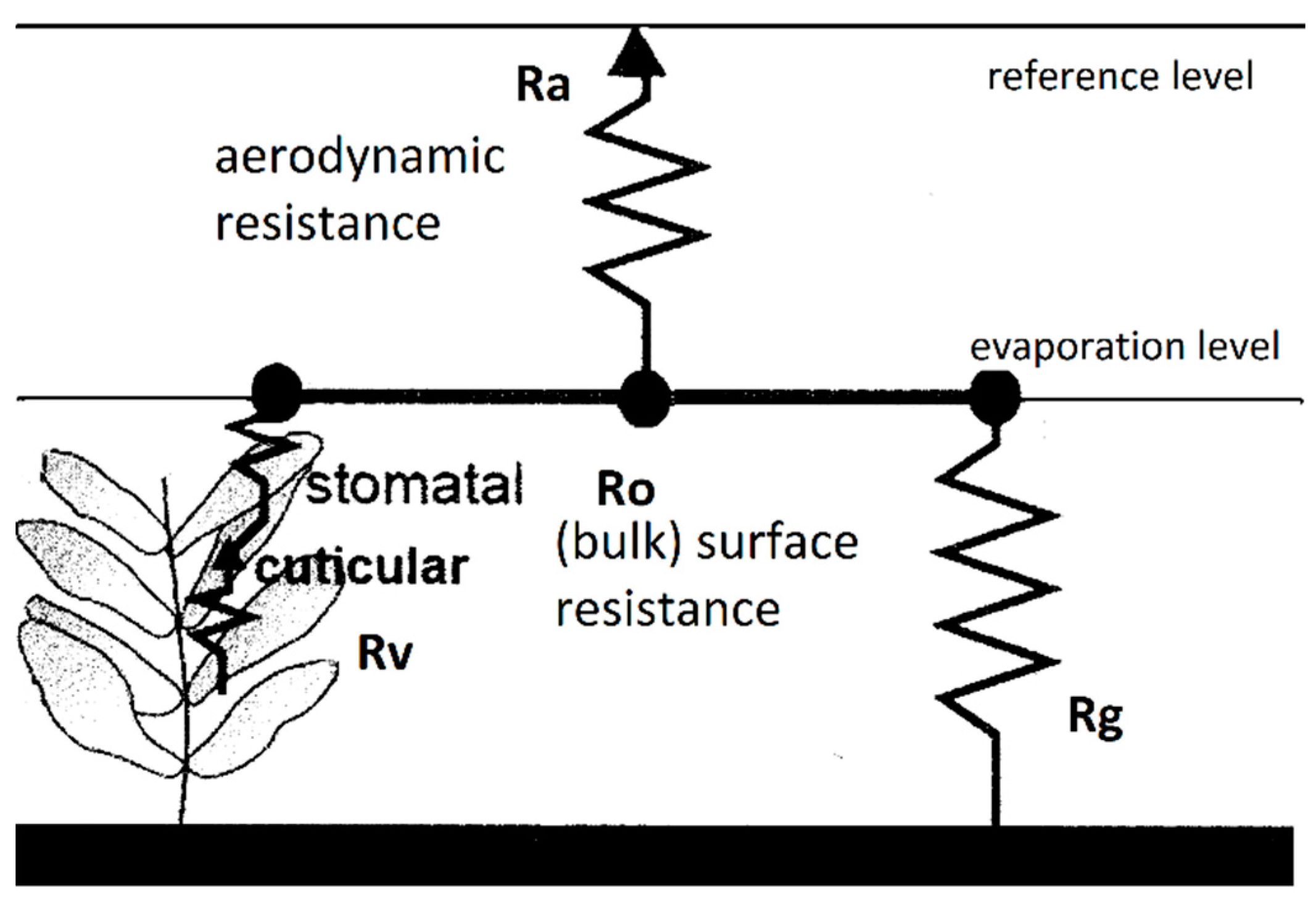
so that  Ra/R0 = (P2UR*)−1+ (P3UC(wsat – w)p/Da)−1
The coefficients P1, P2, P3 were calculated by non-linear minimization of Equation (8).
In this case it is assumed that in partially vegetated areas the bulk surface resistance R0 can be expressed as two independent contributions of the vegetated and the non-vegetated surface fractions. Their resistances, Rv and Rg respectively, are in parallel combination, weighted with the unknown parameters P2 and P3.
CASE (3): The nonlinear regressions in items (1) and (2) were considered again (i.e., parameterization of both Ra and R0 with and without soil moisture contribution) but the minimization procedure was now applied to Equations (10) and (11) instead of (8) and (9). In this case no information about the surface fluxes is needed for the calibration procedure and T0 only is used for the parameter calibration.
In items (2) and (3), when taking into account the soil moisture, some essential characteristics of the soil response should also be known. They were estimated in the same way as Kondo et al. [26], using an experimental set-up of two simultaneous evaporation plates and a precision balance, as mentioned in Section 2, that allow the estimation of the parameter p and the coefficient C in Equation (7), together with the saturation soil moisture wsat (Figure 3).
Figure 3. The two plates experimental arrangement. The plates are 35 cm in diameter and 4 cm in depth and are placed on an insulating sheet. The inserted sensors (thermometer Campbell 107L and soil moisture sensor Decagon EC-5) are also shown, together with the precision balance.
Atmosphere 06 00255 g003
The results are shown in Figure 4, for the experimental data and the regression function F(w) = C(wsat − w)p with wsat = 0.42 ± 0.02 as obtained for the soil saturation moisture in the experiment. The obtained parameters are p = 12 and C = 4500. However an estimate of C is actually not strictly necessary in this application, because a regression coefficient Cs depending on the actual fractional vegetation cover in the experimental site must be always estimated in the model calibration, and C and Cs, could be both included in the regression parameter P3 (Equation (7)).
Both the 2006 and 2009 data sets were divided into two non-overlapping subsets (alternating days), one of them was used for parameter calibration and the other for fluxes calculation with the obtained parameters. The computations are made over hourly averaged data of the turbulent fluxes and the other meteorological variables, P1,P2,P3 being the only model parameters to be estimated.
Figure 4. Plot of the wetness function F(w) used in Equation (7) versus the soil moisture w, as obtained by the two plates evaporation experiment, with soil samples from the experimental site as mentioned in Section 2 and Section 4. The continuous line shows the regression function F(w) = C(wsat – w)p with wsat = 0.42, p = 12 and C = 4500. The point sizes are of the order of their experimental uncertainty.
Atmosphere 06 00255 g004
The results are shown in Table 1 for the obtained parameter values and the statistics of the vapor fluxes comparison, and in Figure 5, Figure 6 and Figure 7 for the calculated fluxes for the 2006 and 2009 data sets.
Figure 5. (a) Calculated versus measured sensible heat flux (hourly data) for year 2006 for case (1); (b) Calculated versus measured sensible heat flux for year 2009 for case (1). Plus signs: flux-gradient method, circles: single parameter linear model, squares: two parameters nonlinear model. The continuous line indicates x = y.
Atmosphere 06 00255 g005
Figure 5a,b show the sensible heat flux Qs calculated by the flux-gradient method, together with the sensible heat flux Qs = E − Qem calculated from the surface energy budget with the latent heat flux Qem obtained for case (1). They are compared with the measured sensible heat fluxes. In the flux-gradient method two constant values of Ch are used after being obtained from Equation (2) averaged over the two data sets respectively with Ra obtained as in Equation (5). They are Ch = 10 ± 6 × 10⁻³ (2006) and Ch = 9 ± 7 × 10⁻³ (2009).
It appears that the use of the PM equation instead of a direct application of the flux-gradient calculations reduces the scatter of the calculated fluxes that is probably due to the uncertainty on the air-surface temperature difference which can be can be quite significant. The PM equation does not make a direct use of the temperature difference to recalculate the fluxes, although this information is contained both in the linear and non-linear regressions of the parameters calibration (see Equations (6) and (8)). The required data input are almost the same for the two methods, with the addition of just the air humidity required only in the PM equation.
Figure 6. (a) Calculated versus measured latent heat flux (hourly data) for year 2006 for case (2); (b) Calculated versus measured latent heat flux for year 2009 for case (2). Circles: two parameters log-linear model, squares: three parameters nonlinear model, plus signs: single parameter linear model of case (1) for comparison. The continuous line indicates x = y.
Atmosphere 06 00255 g006
Figure 6a,b show the calculated latent heat fluxes for case (2) in which the additional information about the soil surface moisture is introduced, together with the results for the first item of case (1) for comparison. Taking into account the soil surface moisture content does not apparently give relevant improvements in the flux estimates. This should imply that the relevant part of the evapotranspiration is related to the permanent vegetation cover in the surrounding areas (evergreen trees) and not to the evaporation from the soil surface. Indeed in the measurement site the soil surface usually exhibits a quick drying up in a few days even after a strong rain event, but leaving a reasonable moisture quantity at few tens of centimeters underground even for very long dry periods. In this way it works as a cover that limits soil evaporation while preserving underground moisture in the root zone, and thus maintaining plant evapotranspiration at the same time. Similar results about the model sensitivity to the soil moisture were found by Stannard [27], also in a semiarid site. The details of the statistical analysis of the regressions are reported in Table 1, where a calculation of the fractional evaporative contribution from the vegetated surface (fev) in the resistance parallel model is also shown (fev = <R0/Rv>, with <…> indicating the average over the data set).
Table 1. Regression parameters and statistics for the calculated versus the measured latent heat fluxes. 1par: one parameter resistance model, 2par: two parameters resistance model, 3par: three parameters resistance model, slope: slope of the regression line through origin, corr: correlation coefficient, sigma: RMS dispersion of the calculated fluxes with respect to the regression line. Calculated parameters P1,P2,P3 with their statistical uncertainties for the non-linear (nl) or linear (lin) regressions, calculated parameters A and p for the logarithmic linear (lin) regressions. Calculated fractional evapotranspiration flux from the vegetation (fev) for the parallel resistance in the three-parameter resistance model.
2006
ModelCaseSigma (W∙m−2)Slopecorr.P1 (Ch,10−3)P2 (10−2)P3 (102)
A(10−2)
pfev
1par, lin(1)270.940.93 3.2 ± 1.5
2par, nl(1)280.990.978 ± 0.43 ± 0.4
2par, lin(2)270.940.93 0.9 −0.57
3par, nl(2)250.950.948.5 ± 0.43.8 ± 0.2170 ± 300 0.99 ±.01
2par, nl(3)250.850.9410 ± 34 ± 3
3par, nl(3)290.820.909 ± 35.1 ± 5.532 ± 36 0.84 ± 0.28
2009
ModelCaseSigma (W∙m−2)slopeCorr.P1 (Ch,10−3)P2 (10−2)P3 (102)
A(10−2)
pfev
1par, lin(1)330.940.93 3.4 ± 2
2par, nl(1)380.970.956.3 ± 0.42.9 ± 0.1
2par, lin(2)301.00.94 −0.31
3par, nl(2)370.920.896.1 ± 0.24.0 ± 0.32.4 ± 0.5 0.89 ± 0.2
2par, nl(3)330.730.877.5 ± 24 ± 3
3par, nl(3)390.880.887.2 ± 1.45.4 ± 3.21.5 ± 0.9 0.84 ± 0.2
In Figure 7a,b the results of the calculated latent heat flux for case 3 are reported. Here no information from measured fluxes is used for calibrations and for this reason the results were also compared with those coming from the application of the method by Venturini et al. [11], that requires no on-site calibration by the surface fluxes and has almost the same input parameters, including the surface brightness temperature, with the exception of the wind speed (and the soil surface moisture when taken into account).
In this case the PM calibrated method gives a smaller bias with respect to Venturini’s method. Table 1 also shows that the scatter and the correlation are worse but still comparable with those of case (1) and (2) (flux calibration), but with a much larger uncertainty for the obtained parameters P1 and P2, that affects the slope of the regression curve. Table 1 also shows that:
-
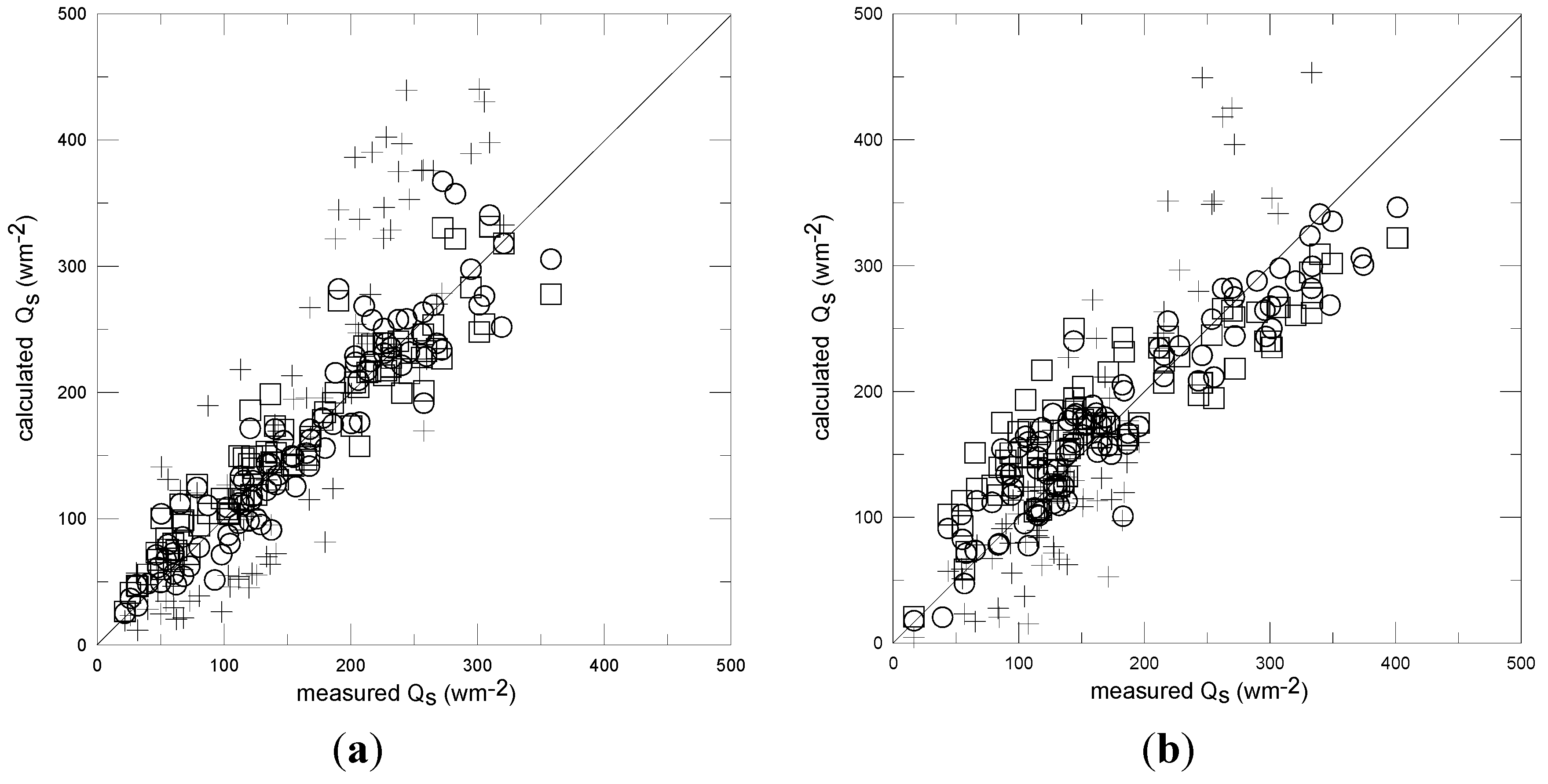
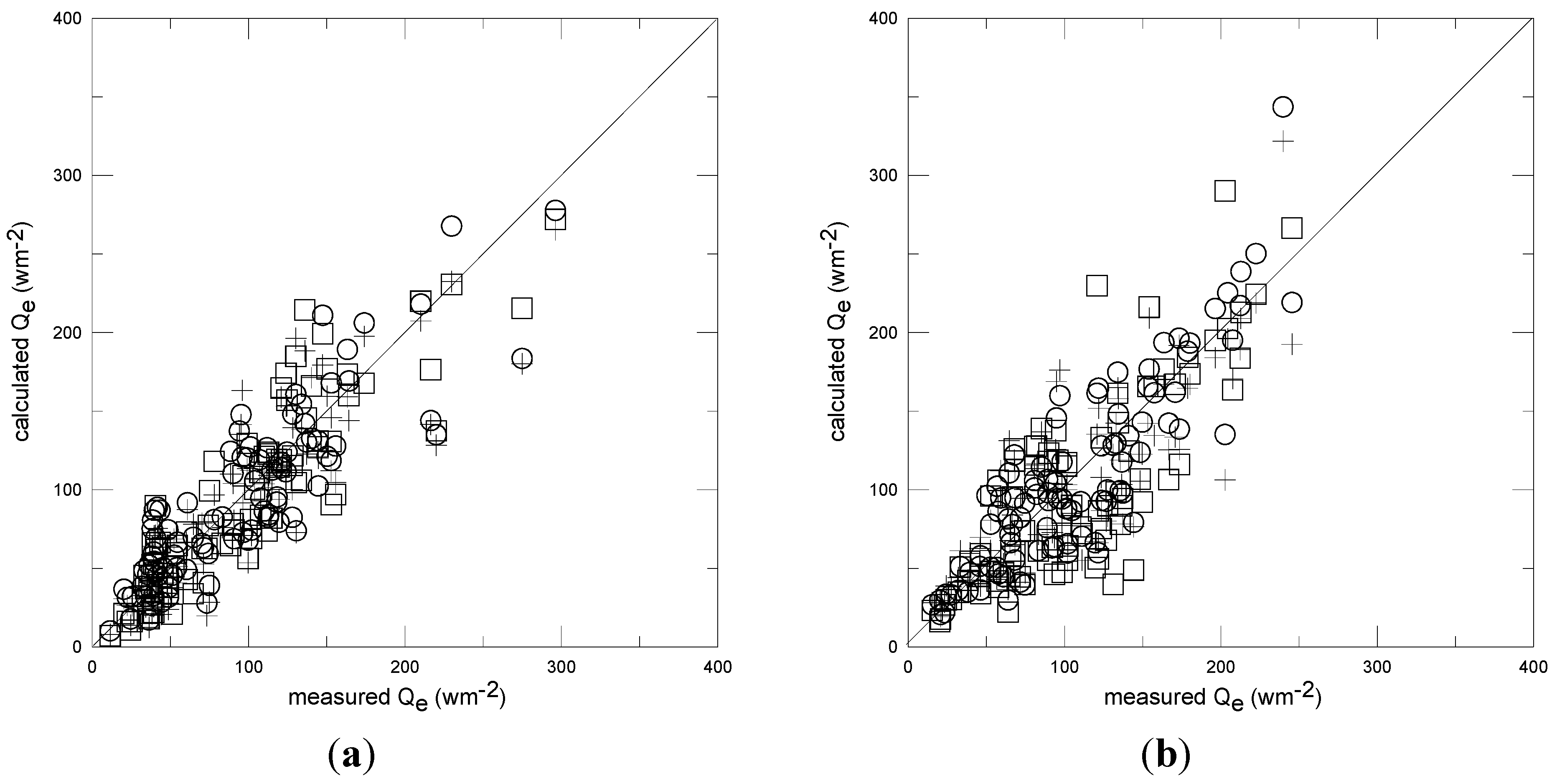
The parameterization of Ch (non-linear regression) adds a little more scatter with respect to the case without parameterization (linear regression), however the effect is small.
-
There are some differences in the parameter P1 between the years 2006 and 2009. This is somehow expected as the resistance model does not contain explicit parameters describing the surface/canopy morphology (e.g., LAI, roughness parameters), thus calibrations are expected to change in time with changes in canopy cover and soil use. In summer 2008 a fire destroyed part of the vegetation cover in the area, and the station was displaced about 200 meters away. The values of parameter P1, (P1, = Ch, that depends on roughness and also stability conditions [14]) show variations from 2006 to 2009 that are larger than their uncertainties in case (1) and (2).
-
The addition of the soil moisture information gives no improvement in 2006 and very little improvement in 2009. This is in agreement with the calculated fractional evaporative contribution by the vegetation (fev, Table 1) and the consequently small bare soil fractional evaporative contribution (1-fev), and with the small sensitivity (large uncertainties) for the calculated parameter P3. Besides changes in the surface cover, the small differences in the effect of the soil moisture between year 2006 and 2009 could be due to differences in precipitation and soil conditions, with about 650 mm annual precipitation and an average aridity index of about 0.35 in 2006, and almost 800 mm precipitation and an (anomalous) aridity index of almost 0.7 in 2009, in the measurement site [38].
-
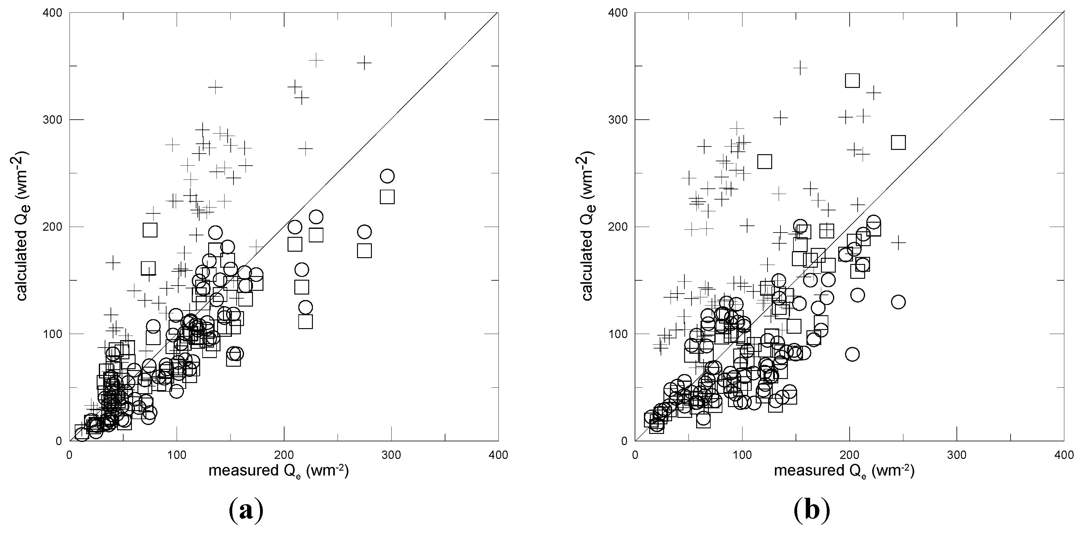
The elimination of the measured fluxes in the calibration procedure (case 3) sensibly increases the statistical uncertainty in the parameter P1 and P2, and this means a smaller sensitivity in the parameter evaluation when the model is calibrated using the surface-air temperature differences only.
Figure 7. (a) Calculated versus measured latent heat flux (hourly data) for year 2006 for case (3); (b) Calculated versus measured latent heat flux for year 2009 for case (3). Circles: two parameters non-linear model, squares: three parameters nonlinear model, plus signs: Venturini’s (2008) model results for comparison. The continuous line indicates x = y.
Atmosphere 06 00255 g007

4. Summary and Conclusions

An approach based on the PM equation was used to estimate the evaporation flux over non-homogeneous terrain in a Mediterranean site in the south east of Italy for two six month data sets from the years 2006 and 2009.
Some expressions for the surface resistance, all based on the “critical resistance” approach were used in the PM equation with either one, two, or three regression parameters. The parameters were calibrated with the latent heat flux and the air-surface temperature difference data, and an attempt was also made to use the temperature differences only. The main conclusions are the following.
(1)
The results compare favorably with those from a flux-gradient method that uses a value of the heat transfer coefficient Ch, calibrated on the same set of input data. In this case the use of the PM equation avoids the introduction of possibly quite large uncertainties coming from the direct use of surface-air temperature gradients.
(2)
The proposed expressions for the aerodynamic and surface resistances do not contain explicit parameters describing the surface/canopy morphology (e.g., LAI, roughness parameters). As a consequence the calibrated model parameters should be used during time periods limited by the morphological surface changes, then recalibrated.
(3)
The information about the surface soil moisture gave very little improvement to the results, only in 2009, a year of enhanced precipitations and anomalous surface moisture conditions, after a little displacement of the station and some differences in vegetation cover with respect to 2006. Although combined resistance models have proven to be generally more successful in modelling evapotranspiration in mixed surface areas [26,27], the surface soil moisture contribution does not seem to be essential for evapotranspiration modelling in the considered site. Here most of the evapotranspiration is likely to be due to the evergreen arboreous vegetation transfer of moisture from the root zone underground, that is often decoupled from the surface moisture. Thus parameter P3 appears large and fairly uncertain, especially in 2006.
(4)
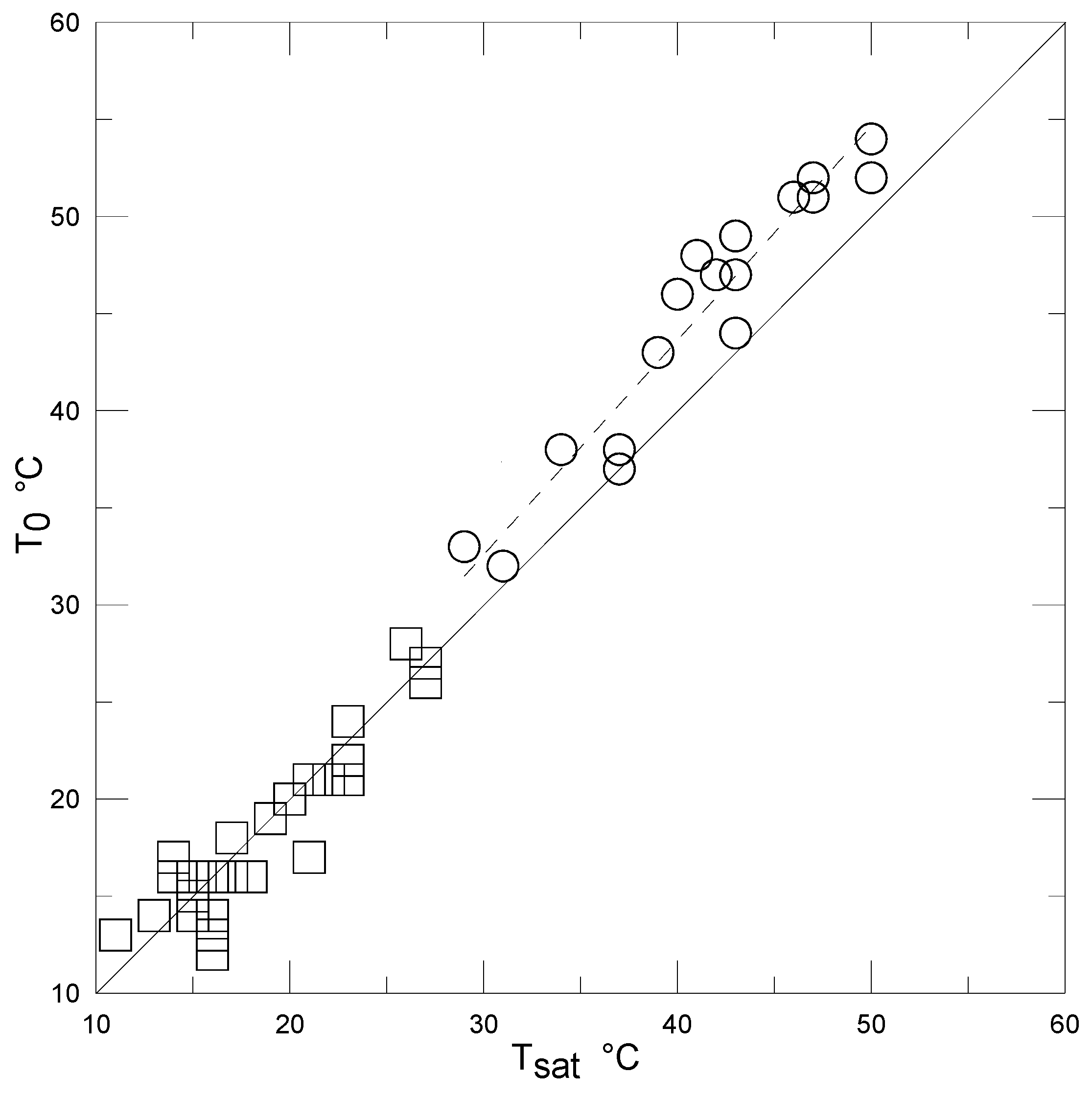
The calculated fluxes showed less accurate but still fairly reasonable results when the calibration was made with respect to the air-surface temperature differences only, with no information about measured fluxes being used. It gives better results than a “complementarity principle” based method, that similarly requires no local flux calibration and is based on the same input data. The calibration with the local temperature appears to reduce the bias in the PM model. However, the statistical uncertainty of the parameter calibration increases considerably, indicating a significant decrease of the sensitivity of the model parameters in this case, compared with the calibration with the local fluxes, and affecting the slope of the regression curve. Thus the applicability of this procedure to other data sets in different conditions requires further investigations.

Acknowledgments

The author strongly acknowledges Cosimo Elefante and Fabio M. Grasso for their help in the management of the experimental base and the data archive. Acknowledgements are due also to Gian P. Marra for providing the satellite temperature data.

Conflicts of Interest

The author declares no conflict of interest.

References

  1. Wang, K.; Dickinson, R.E. A review of global terrestrial evapotranspiration: Observation, modelling, climatology, and climatic variability. Rev. Geophys. 2012, 50, 1–54. [Google Scholar] [CrossRef]
  2. Norman, J.M.; Becker, F. Terminology in thermal infrared remote sensing of natural surfaces. Agric. For. Meteorol. 1995, 77, 153–166. [Google Scholar] [CrossRef]
  3. Kalma, J.D.; McVicar, T.M.; McCabe, M.F. Estimating land surface evaporation: A review of methods using remotely sensed surface temperature data. Surv. Geophys. 2008, 29, 421–469. [Google Scholar] [CrossRef]
  4. Bastiaanssen, W.G.M.; Menenti, M.; Feddes, R.A.; Holsltag, A.A.M. A remote sensing surface energy balance algorithm for land. I. Formulation. J. Hydrol. (Amst.) 1998, 212/213, 198–212. [Google Scholar]
  5. Roerink, G.J.; Su, Z.; Menenti, M. S-SEBI a simple remote sensing algorithm to estimate the surface energy balance. Phys. Chem. Earth Part. B Hydrol. Oceans Atmos. 2000, 25, 147–157. [Google Scholar] [CrossRef]
  6. Noilhan, J.; Planton, S. A simple parameterization of land surface processes for meteorological models. Mon. Weather Rev. (Amst.) 1988, 117, 536–549. [Google Scholar] [CrossRef]
  7. Coudert, B.; Otttlé, C.; Boudevillain, B.; Demarty, J.; Guillevic, P. Contribution of thermal infrared remoste sensing data in multiobjective calibration in a dual source SVAT model. J. Hydrometeorol. 2006, 7, 404–420. [Google Scholar] [CrossRef]
  8. Su, Z. The Surface Energy Balance System (SEBS) for estimation of turbulent heat fluxes. Hydrol. Earth Syst. Sci. 2002, 6, 85–99. [Google Scholar] [CrossRef]
  9. Norman, J.M.; Kustas, W.P.; Humes, K.S. A two-source approach for estimating soil and vegetation energy fluxes from observations of directional radiometric surface temperature. Agric. For. Meteorol. 1995, 77, 263–293. [Google Scholar] [CrossRef]
  10. Granger, R.J. A complementarity relationship approach for evaporation from non-saturated surfaces. J. Hydrol. (Amst.) 1989, 111, 31–38. [Google Scholar] [CrossRef]
  11. Venturini, V.; Islam, S.; Rodriguez, L. Estimation of evaporative fraction and evapotranspiration from MODIS products using a complementary based model. Remote Sens. Eviron. 2008, 112, 132–141. [Google Scholar] [CrossRef]
  12. Stewart, J.B. Turbulent surface fluxes derived from radiometric surface temperature of sparse prairie grass. J. Geophys. Res. 1995, 100, 25429–25433. [Google Scholar] [CrossRef]
  13. Cooper, J.H.; Smith, E.A. Limitations in estimating surface sensible heat fluxes from surface and satellite radiometric skin temperatures19. J. Geophys. Res. 1995, 100, 25419–25427. [Google Scholar] [CrossRef]
  14. Garratt, J.R. The Atmospheric Boundary Layer; Cambridge University Press: Cambridge, UK, 1992; p. 316. [Google Scholar]
  15. Allen, R.G.; Pereira, L.S.; Raes, D.; Smith, M. Crops Evapotranspiration: Guidelines for Computing Crop Water Requirements; FAO Irrigation and Drainage Paper 56; FAO: Rome, Italy, 1998; p. 300. [Google Scholar]
  16. Allen, R.G.; Pruitt, W.O.; Wright, J.L.; Howell, T.A.; Ventura, F.; Snyder, R.; Itenfisu, D.; Steduto, P.; Berengena, J.; Yrisarry, J.B.; et al. A recommendation on standardized surface resistance for hourly calculation of reference ET0 by the FAO 56 Penmann-Monteith method. Agric. Water Manag. 2006, 81, 1–22. [Google Scholar] [CrossRef]
  17. Glenn, E.P.; Neale, C.M.U.; Hunsaker, D.J.; Nagler, P.L. Vegetation index-based crop coefficients to estimate evapotranspiration by remote sensing in agricultural and natural ecosystems. Hydrol. Process. 2011, 25, 4050–4062. [Google Scholar] [CrossRef]
  18. Nagler, P.L.; Glenn, E.P.; Nguyen, U.; Scott, R.L.; Doody, T. Estimating riparian and agricultural actual evapotranspiration by reference evapotranspiration and MODIS Enhanced Vegetation Index. Remote Sens. 2013, 5, 3849–3871. [Google Scholar] [CrossRef]
  19. Alves, I.; Pereira, L.S. Modelling surface resistance from climatic variables? Agric. Water Manag. 2000, 42, 371–385. [Google Scholar] [CrossRef]
  20. Jarvis, P.G. The interpretation of the variations in leaf water potential and stomatal conductance found in canopies in the field. Phil. Trans. R. Soc. Lond. B 1976, 273, 593–610. [Google Scholar] [CrossRef]
  21. Katerji, N.; Perrier, A. Modélisation de l’évapotranpsiration réelle ETR d’une parcelle de luzerne: Rôle d’un coefficient cultural. Agronomie 1983, 3, 513–521. [Google Scholar] [CrossRef]
  22. Rana, G.; Katerji, N.; Mastrorilli, M.; El Moujabber, M.A. Model for predicting actual evapotranspiration under water stress conditions in a Mediterranean region. Theor. Appl. Climatol. 1997, 56, 45–55. [Google Scholar] [CrossRef]
  23. Rana, G.; Katerji, N.; Mastrorilli, M. Environmental soil-plant parameters for modelling actual crop evapotranspiration under water stress conditions. Ecol. Model. 1997, 101, 363–371. [Google Scholar] [CrossRef]
  24. Katerji, N.; Rana, G. Modelling evapotranspiration of six irrigated crops under Mediterranean climate conditions. Agric. For. Meteorol. 2006, 138, 142–155. [Google Scholar] [CrossRef]
  25. Stewart, J.B. Modelling surface conductance of pine forest. Agric. For. Meteorol. 1988, 43, 19–35. [Google Scholar] [CrossRef]
  26. Shuttleworth, J.; Wallace, J.S. Evaporation from sparse crops—An energy combination theory. Quart. J. Roy. Meteorol. Soc. 1985, 111, 839–855. [Google Scholar] [CrossRef]
  27. Stannard, D.I. Comparison of Penman-Monteith, Shuttleworth-Wallace, and modified Priestley-Taylor evapotranspiration models for wildland vegetation in semiarid rangeland. Water Resources Res. 1993, 29, 1379–1392. [Google Scholar] [CrossRef]
  28. Tsengdar, J.L.; Pielke, R.A. Estimating the soil surface specific humidity. J. Appl. Meteorol. 1992, 31, 480–484. [Google Scholar] [CrossRef]
  29. Kondo, J.; Saigusa, N.; Sato, T. A parameterization of evaporation from bare soil surfaces. J. Appl. Meteorol. 1990, 29, 385–389. [Google Scholar] [CrossRef]
  30. Basesperimentale. Available online: http://www.basesperimentale.le.isac.cnr.it/ (accessed on 16 February 2015).
  31. Martano, P.; Elefante, C.; Grasso, F. A database for long term atmosphere-surface transfer monitoring in Salento Peninsula (Southern Italy). Dataset Papers Geosci. 2013, 2013, 946431. [Google Scholar] [CrossRef]
  32. Decagon Devices. Available online: http://www.decagon.com/education/calibrating-ech2o-soil-moisture-sensors-13393-04-an/ (accessed on 16 February 2015).
  33. Everest Interscience Inc. Available online: http://www.everestinterscience.com/products/Enviro-Therm/Enviro-Therm.htm (accessed on 16 February 2015).
  34. Beck, J.V.; Arnold, K.J. Parameter Estimation in Engineering and Science; Wiley: New York, NY, USA, 1977. [Google Scholar]
  35. Martano, P. Inverse parameter estimation of the turbulent surface layer from single-level data and surface temperature. J. Appl. Meteorol. 2008, 47, 1027–1037. [Google Scholar] [CrossRef]
  36. Cava, D.; Contini, D.; Donateo, A.; Martano, P. Analysis of short-term closure of the surface energy balance above short vegetation. Agric. For. Meteorol. 2008, 148, 82–93. [Google Scholar] [CrossRef]
  37. The World Data Center for Remote Sensing in the Atmosphere. Available online: http://wdc.dlr.de/data_products/SURFACE/land_surface_temperature.php (accessed on 16 February 2015).
  38. Martano, P.; Elefante, C.; Grasso, F. Ten years surface water and energy balance from the ISAC micrometeorological station in Salento peninsula (southern Italy). Adv. Sci. Res. 2014. submitted. [Google Scholar]

