
PM2.5 Concentration Differences between Various Forest Types and Its Correlation with Forest Structure


Abstract
:1. Introduction
2. Methods
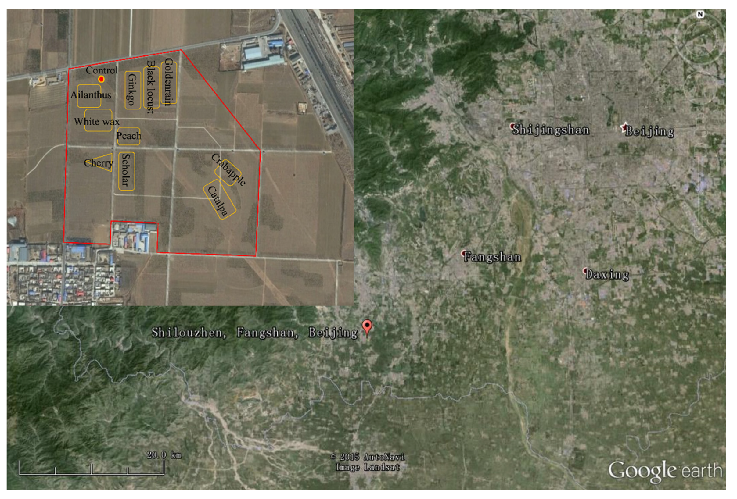
2.1. Sampling Site


| Stages | Control | Crabapple | Cherry | Peach | Ailanthus | Scholar | Catalpa | White Wax | Black Locust | Goldenrain | Ginkgo | |
|---|---|---|---|---|---|---|---|---|---|---|---|---|
| DBH (cm) | LEP | 0 | 2.55 | 5.50 | 5.65 | 8.00 | 7.45 | 5.86 | 7.07 | 8.62 | 7.55 | 6.80 |
| LOP | 0 | 2.68 | 5.93 | 6.03 | 8.60 | 8.03 | 6.17 | 7.44 | 9.23 | 7.82 | 7.15 | |
| DP | 0 | 2.70 | 6.00 | 6.15 | 8.60 | 8.10 | 6.22 | 7.50 | 9.33 | 7.99 | 7.15 | |
| Height (m) | LEP | 0 | 1.66 | 2.49 | 3.00 | 4.20 | 5.11 | 3.30 | 5.00 | 5.20 | 5.40 | 7.25 |
| LOP | 0 | 1.75 | 2.79 | 3.11 | 4.10 | 5.59 | 3.51 | 5.55 | 6.04 | 5.79 | 7.72 | |
| DP | 0 | 2.05 | 3.09 | 3.41 | 4.40 | 5.89 | 3.81 | 5.85 | 6.34 | 6.09 | 8.02 | |
| Canopy Density | LEP | 0 | 0.10 | 0.25 | 0.58 | 0.11 | 0.20 | 0.15 | 0.38 | 0.65 | 0.45 | 0.16 |
| LOP | 0 | 0.15 | 0.39 | 0.83 | 0.20 | 0.40 | 0.23 | 0.57 | 0.90 | 0.68 | 0.19 | |
| DP | 0 | 0.10 | 0.20 | 0.42 | 0.10 | 0.18 | 0.16 | 0.25 | 0.40 | 0.34 | 0.15 | |
| LAI | LEP | 0 | 0.90 | 2.40 | 3.00 | 1.00 | 2.34 | 1.40 | 2.60 | 3.25 | 2.76 | 0.80 |
| LOP | 0 | 1.17 | 3.18 | 4.12 | 1.52 | 2.78 | 1.92 | 3.71 | 4.62 | 3.54 | 0.97 | |
| DP | 0 | 0.78 | 1.63 | 2.08 | 0.76 | 1.25 | 1.34 | 1.63 | 2.05 | 1.77 | 0.77 | |
| Forestland Area (m2) | 1901 | 2098 | 1898 | 1699 | 4162 | 4076 | 3596 | 2664 | 3197 | 3197 | 3303 | |
| Herb Height (m) | LEP | 0.28 | 0.33 | 0.10 | 0.10 | 0.27 | 0.32 | 0.45 | 0.44 | 0.38 | 0.38 | 0.42 |
| LOP | 0.60 | 0.50 | 0.20 | 0.10 | 0.40 | 0.50 | 0.65 | 0.60 | 0.55 | 0.55 | 0.60 | |
| DP | 0 | 0 | 0.05 | 0.05 | 0 | 0 | 0 | 0 | 0 | 0 | 0.05 | |
| Herb Cover | LEP | 70% | 30% | 5% | 5% | 41% | 37% | 52% | 49% | 48% | 48% | 50% |
| LOP | 90% | 35% | 5% | 8% | 50% | 45% | 65% | 60% | 55% | 55% | 60% | |
| DP | 0% | 0% | 5% | 8% | 0% | 0% | 0% | 0% | 0% | 0% | 5% | |
| Number of Tree | 0 | 49 | 49 | 49 | 25 | 25 | 25 | 25 | 25 | 25 | 25 | |
2.2. Sampling
2.3. Analysis
3. Results and Discussion
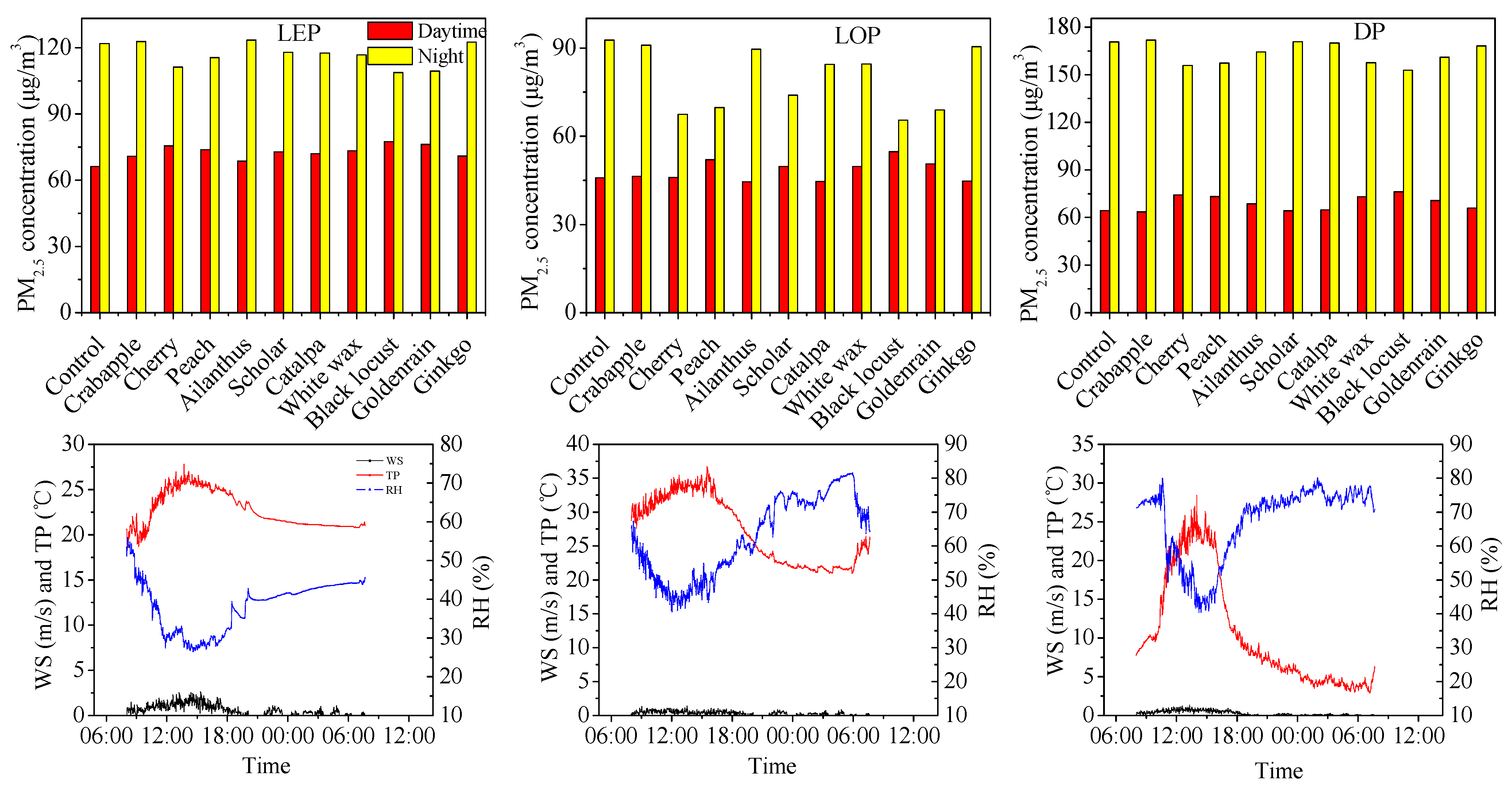
3.1. PM2.5 Concentration Differences at Different Times
| Leaf Expansion Period | Leaf Flourish Period | Deciduous Period | |||||||
|---|---|---|---|---|---|---|---|---|---|
| Daytime | Night | Total | Daytime | Night | Total | Daytime | Night | Total | |
| Crabapple | −7.04 | −0.70 | −2.93 | −1.07 | 1.85 | 0.89 | 1.10 | 0.66 | 0.79 |
| Cherry | −14.04 | 8.81 | 0.77 | −0.31 | 11.02 | 7.27 | −15.34 | 8.96 | 2.32 |
| Peach | −11.43 | 5.28 | −0.60 | −13.36 | 13.92 | 4.89 | −13.89 | 8.84 | 2.63 |
| Ailanthus | −3.64 | −1.20 | −2.06 | 2.96 | 3.28 | 3.18 | −6.66 | 4.76 | 1.64 |
| Scholar | −9.98 | 3.30 | −1.37 | −8.44 | 20.17 | 10.70 | 0.14 | -0.68 | −0.45 |
| Catalpa | −8.70 | 3.61 | −0.72 | 2.66 | 8.87 | 6.82 | −0.68 | 0.75 | 0.36 |
| White wax | −10.71 | 4.29 | −0.99 | −8.39 | 8.73 | 3.07 | −13.64 | 8.20 | 2.23 |
| Black locust | −17.00 | 10.80 | 1.01 | −19.37 | 29.37 | 13.24 | −18.48 | 9.44 | 1.81 |
| Goldenrain | −15.12 | 10.28 | 1.34 | −10.43 | 25.60 | 13.68 | −10.00 | 6.48 | 1.98 |
| Ginkgo | −7.20 | −0.47 | −2.84 | 2.46 | 2.41 | 2.43 | −2.72 | 2.54 | 1.10 |
3.2. Differences in the PM2.5 Concentration Index between the Different Forests
3.3. Effect of Climatic Conditions on PM2.5 Concentration
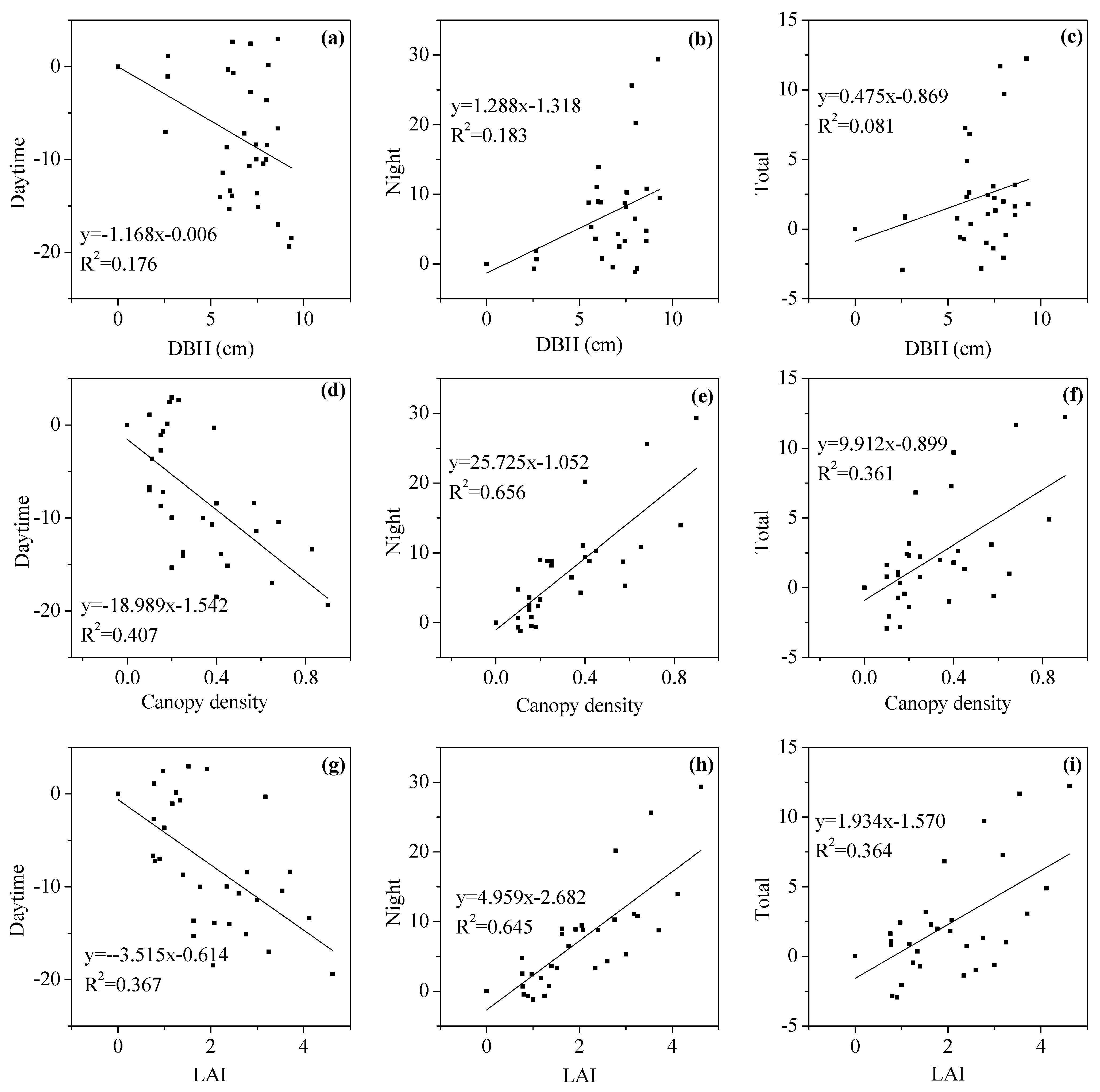
3.4. Correlation between the PM2.5 Concentration Index and Forest Structure
| DBH | Height | Canopy Density | LAI | Forestland Area | Herb Height | Herb Cover | ||
|---|---|---|---|---|---|---|---|---|
| LEP | Daytime | −0.427 | −0.427 | −0.936 ** | −0.918 ** | 0.223 | 0.316 | 0.088 |
| Night | 0.264 | 0.255 | 0.855 ** | 0.855 ** | −0.360 | −0.330 | −0.084 | |
| Total | 0.155 | 0.055 | 0.573 * | 0.609 * | −0.351 | −0.223 | 0.042 | |
| LOP | Daytime | −0.245 | −0.255 | −0.791 ** | −0.773 ** | 0.383 | 0.416 | 0.325 |
| Night | 0.609 * | 0.509 | 0.909 ** | 0.836 ** | 0.096 | −0.475 | −0.297 | |
| Total | 0.621 * | 0.491 | 0.773 ** | 0.691 * | 0.232 | −0.393 | −0.261 | |
| DP | Daytime | −0.304 | −0.247 | −0.665 ** | −0.628 ** | 0.289 | 0.216 | 0.183 |
| Night | 0.385 * | 0.255 | 0.861 ** | 0.853 ** | −0.170 | 0.135 | 0.179 | |
| Total | 0.381 * | 0.268 | 0.616 ** | 0.554 ** | −0.050 | 0.233 | 0.250 | |
| Total | Daytime | −0.323 | −0.247 | −0.665 ** | −0.628 ** | 0.289 | 0.216 | 0.144 |
| Night | 0.377 * | 0.246 | 0.848 ** | 0.832 ** | −0.184 | 0.105 | 0.147 | |
| Total | 0.356 * | 0.263 | 0.583 ** | 0.517 ** | −0.053 | 0.226 | 0.218 | |

4. Conclusions and Recommendations for Application
Acknowledgments
Author Contributions
Conflicts of Interest
References
- Xiao, Q.F.; McPherson, E.G.; Simpson, J.R. Rainfall interception by Sacramento’s urban forest. J. Arboric. 1998, 24, 235–244. [Google Scholar]
- Akbari, H.; Konopacki, S. Calculating energy-saving potentials of heat-island reduction strategies. Energy Policy 2005, 33, 721–756. [Google Scholar] [CrossRef]
- McPherson, E.G. Atmospheric carbon dioxide reduction by Sacramento’s urban forest. J. Arboric. 1998, 24, 215–223. [Google Scholar]
- McPherson, E.G.; Simpson, J.R. Air pollutant uptake by Sacramento’s urban forest. J. Arboric. 1998, 24, 224–234. [Google Scholar]
- Nowak, D.J.; Crane, D.E.; Stevens, J.C. Air pollution removal by urban trees and shrubs in USA. Urban For. Urban Green. 2006, 4, 115–123. [Google Scholar] [CrossRef]
- Wu, Z.P.; Wang, C.; Xu, J.N.; Hu, L.X. Air-borne anions and particulate matter in six urban green spaces during the summer. J. Tsinghua Univ. Sci. Technol. 2007, 47, 2152–2157. [Google Scholar]
- Yang, J.; McBride, J.; Zhou, J.; Sun, Z. The urban forest in Beijing and its role in air pollution reduction. Urban For. Urban Green. 2005, 3, 65–78. [Google Scholar] [CrossRef]
- Beijing Municipal Bureau of Environmental Protection Environmental Quality. Available online: http://www.bjepb.gov.cn/bjepb/413526/331443/331937/333896/425596/index.html (accessed on 3 November 2015).
- Myhre, G. Consistency between satellite-derived and modeled estimates of the direct aerosol effect. Science 2009, 325, 187–190. [Google Scholar] [CrossRef] [PubMed]
- McDonald, A.G.; Bealey, W.J.; Fowler, D.; Dragosits, U.; Skiba, U.; Smith, R.I. Quantifying the effect of urban tree planting on concentrations and depositions of PM10 in two UK conurbations. Atmos. Environ. 2007, 41, 8455–8467. [Google Scholar] [CrossRef]
- Janne, R.V.; Pasi, Y.P.; Holopainen, T.; Jorma, J.; Pertti, P.; Minna, K. Soil drought increases atmospheric fine particle capture efficiency of Norway spruce. Boreal Environ. Res. 2012, 17, 21–30. [Google Scholar]
- Beckett, P.K.; Freer-Smith, P.H.; Taylor, G. Particulate pollution capture by urban trees: Effects of species and wind speed. Glob Chang. Biol. 2000, 6, 995–1003. [Google Scholar] [CrossRef]
- Freer-Smith, P.H.; El-Khatib, A.A.; Taylor, G. Capture of Particulate Pollution by trees: A comparison of species typical of semi-arid areas (Ficus nitida and Eucalyptus globulus) with European and North American species. Water Air Soil Pollut. 2004, 155, 173–187. [Google Scholar] [CrossRef]
- Freer-Smith, P.H.; Beckett, P.K.; Taylor, G. Deposition velocities to Sorbus aria, Acer Campestre, Populus deltoids × trichocarpa “Beaupré”, Pinus nigra × Cupressocyparis leylandii for coarse, fine and ultra-fine particles in the urban environment. Environ. Pollut. 2005, 133, 157–167. [Google Scholar] [CrossRef] [PubMed]
- Litschke, T.; Kuttler, W. On the reduction of urban particle concentration by vegetation—a review. Meteorol. Z. 2008, 17, 229–240. [Google Scholar] [CrossRef]
- Acero, J.A.; Simon, A.; Padro, A.; Santa Coloma, O. Impact of local urban design and traffic restrictions on air quality in a medium-sized town. Environ. Technol. 2012, 33, 2467–2477. [Google Scholar] [CrossRef] [PubMed]
- Liu, Y.S.; Shen, X.X.; Mao, X.L.; Chen, R. Indoor air levels of TSP, PM10, PM2.5 and PM1 at public places in Beijing during wintertime. Acta Sci. Agron. 2004, 24, 190–196. [Google Scholar]
- Benjamin, M.T.; Winer, A.M. Estimating the ozone forming potential of urban trees and shrubs. Atmos. Environ. 1998, 32, 53–68. [Google Scholar] [CrossRef]
- Beckett, K.P.; Freer-Smith, P.; Taylor, G. Urban woodlands: Their role in reducing the effects of particulate pollution. Environ. Pollution. 1998, 99, 347–360. [Google Scholar] [CrossRef]
- Nowak, D.J.; Crane, D.E.; Stevens, J.C.; Hoehn, R.E.; Walton, J.T.; Bond, J. A ground-based method of assessing urban forest structure and ecosystem services. Arbori. Urban For. 2008, 34, 347–358. [Google Scholar]
- Santosh, K.P. Ecological effect of airborne particulate matter on plants. Environ. Skept. Crit. 2012, 1, 12–22. [Google Scholar]
- Zhou, X.W.; Kang, X.P. Study on dust-retention ability of different green plants on campus. J. Anhui Agric. Sci. 2008, 36, 10431–10432. [Google Scholar]
- Dzierżanowski, K.; Popek, R.; Gawrońska, H.; Sæbø, A.; Gawroński, S.W. Deposition of particulate matter of different size fractions on leaf surfaces and in waxes of urban forest species. Int. J. Phytorem. 2011, 13, 1037–1046. [Google Scholar] [CrossRef] [PubMed]
- Popek, R.; Gawrońska, H.; Sæbø, A.; Wrochna, M.; Gawroński, S.W. Particulate matter on foliage of 13 woody species: Deposition on surfaces and phytostabilisation in waxes: A 3-year study. Int. J. Phytorem. 2013, 15, 245–256. [Google Scholar] [CrossRef] [PubMed]
- Determination of atmospheric articles PM10 and PM2.5 in ambient air by gravimetric method. Available online: http://kjs.mep.gov.cn/hjbhbz/bzwb/dqhjbh/jcgfffbz/201109/t20110914_217272.htm (accessed on 5 November 2015).
- Nguyen, T.; Yu, X.X.; Zhang, Z.M.; Liu, M.M.; Liu, X.H. Relationship between types of urban forest and PM2.5 capture at three growth stages of leaves. J. Environ. Sci. 2015, 27, 33–41. [Google Scholar] [CrossRef] [PubMed]
- Zhao, C.X.; Wang, Y.Q.; Wang, Y.J.; Zhang, H.L. Temporal and Spatial Distribution of PM2.5 and PM10 Pollution status and the correlation of particulate matters and meteorological factors during winter and spring in Beijing. Environ. Sci. 2014, 35, 418–427. (In Chinese) [Google Scholar]
- Pathak, R.K.; Wu, W.S.; Wang, T. Summertime PM2.5 ionic species in four major cities of China: Nitrate formation in an ammonia-deficient atmosphere. Atmos. Chem. Phys. 2009, 9, 1711–1722. [Google Scholar] [CrossRef]
- Rasheed, A.; Aneja, V.P.; Aiyyer, A.; Rafique, U. Measurement and analysis of fine particulate matter (PM2.5) in urban areas of Pakistan. Aerosol Air Qual. Res. 2015, 15, 426–439. [Google Scholar] [CrossRef]
- Li, Y.; Chen, Q.; Zhao, H.; Wang, L.; Tao, R. Variations in PM10, PM2.5 and PM1.0 in an Urban Area of the Sichuan Basin and their relation to meteorological factors. Atmosphere 2015, 6, 150–163. [Google Scholar] [CrossRef]
- Fowler, D.; Cape, J.N.; Unsworth, M.H.; Mayer, H.; Crowther, J.M.; Jarvis, P.G.; Shuttleworth, W.J. Deposition of atmospheric pollutants on forests and discussion. Philos. Trans. Royal Soc. B: Biol. Sci. 1989, 324, 247–265. [Google Scholar] [CrossRef]
- Chang, C.R.; Li, M.H.; Chang, C.R.; Li, M.H. Effects of urban parks on the local urban thermal environment. Urban For. Urban Green. 2014, 13, 672–681. [Google Scholar] [CrossRef]
- Sæbø, A.; Popek, R.; Nawrot, B.; Hanslin, H.M.; Gawronska, H.; Gawronski, S.W. Plant species differences in particulate matter accumulation on leaf surfaces. Sci. Total Environ. 2012, 427, 347–354. [Google Scholar] [CrossRef] [PubMed]
- Curtis, A.J.; Helmig, D.; Baroch, C.; Daly, R.; Davis, S. Biogenic volatile organic compound emissions from nine tree species used in an urban tree-planting program. Atmos. Environ. 2014, 95, 634–643. [Google Scholar] [CrossRef]
- Bennett, J.W.; Hung, R.; Lee, S.; Padhi, S. 18 Fungal and bacterial volatile organic compounds: An overview and their role as ecological signaling agents. Fungal Assoc. 2012, 2012, 373–393. [Google Scholar]
- Jacob, D.J.; Winner, D.A. Effect of climate change on air quality. Atmos. Environ. 2009, 43, 51–63. [Google Scholar] [CrossRef]
- Tai, A.P.K.; Mickley, L.J.; Jacob, D.J. Correlation between fine particulate matter (PM2.5) and meteorological variables in USA: Implications for the sensibility of PM2.5 to climate change. Atmos. Environ. 2010, 44, 3976–3984. [Google Scholar] [CrossRef]
- Aw, J.; Kleeman, M.J. Evaluating the first-order effect of interannual temperature variability on urban air pollution. J. Geophys. Res. 2003, 108, 4365. [Google Scholar] [CrossRef]
- Kleeman, M.J. A preliminary assessment of the sensitivity of air quality in California to global change. Clim. Chang. 2008, 87, 273–292. [Google Scholar] [CrossRef]
- Liu, Y.; Paciorek, C.J.; Koutrakis, P. Estimating regional spatial and temporal variability of PM concentrations using satellite data, meteorology, and land use information. Environ. Health Perspect. 2009, 117, 886–892. [Google Scholar] [CrossRef] [PubMed]
- Smith, W.H.; Staskawicz, B.J. Removal of atmospheric particles by leaves and twigs of urban trees: Some preliminary observations and assessment of research needs. Environ. Manag. 1977, 1, 317–330. [Google Scholar] [CrossRef]
- Winkler, P. The growth of atmospheric aerosol particles with relative humidity. Phys. Scr. 1988, 37, 223–230. [Google Scholar] [CrossRef]
- Tallis, M.; Taylor, G.; Sinnett, D.; Freer-Smith, P. Estimating the removal of atmospheric particulate pollution by the urban tree canopy of London, under current and future environments. Landsc. Urban Plan. 2011, 103, 129–138. [Google Scholar] [CrossRef]
- Watson, D.J. Comparative physiological studies on the growth of field crops: I. Variation in net assimilation rate and leaf area between species and varieties and within and between years. Ann. Bot. 1947, 11, 41–76. [Google Scholar] [CrossRef]
© 2015 by the authors; licensee MDPI, Basel, Switzerland. This article is an open access article distributed under the terms and conditions of the Creative Commons Attribution license (http://creativecommons.org/licenses/by/4.0/).
Share and Cite
Liu, X.; Yu, X.; Zhang, Z. PM2.5 Concentration Differences between Various Forest Types and Its Correlation with Forest Structure. Atmosphere 2015, 6, 1801-1815. https://doi.org/10.3390/atmos6111801
Liu X, Yu X, Zhang Z. PM2.5 Concentration Differences between Various Forest Types and Its Correlation with Forest Structure. Atmosphere. 2015; 6(11):1801-1815. https://doi.org/10.3390/atmos6111801
Chicago/Turabian StyleLiu, Xuhui, Xinxiao Yu, and Zhenming Zhang. 2015. "PM2.5 Concentration Differences between Various Forest Types and Its Correlation with Forest Structure" Atmosphere 6, no. 11: 1801-1815. https://doi.org/10.3390/atmos6111801
APA StyleLiu, X., Yu, X., & Zhang, Z. (2015). PM2.5 Concentration Differences between Various Forest Types and Its Correlation with Forest Structure. Atmosphere, 6(11), 1801-1815. https://doi.org/10.3390/atmos6111801