
Combining DMSP/OLS Nighttime Light with Echo State Network for Prediction of Daily PM2.5 Average Concentrations in Shanghai, China

Abstract
:1. Introduction
2. Study Area and Data
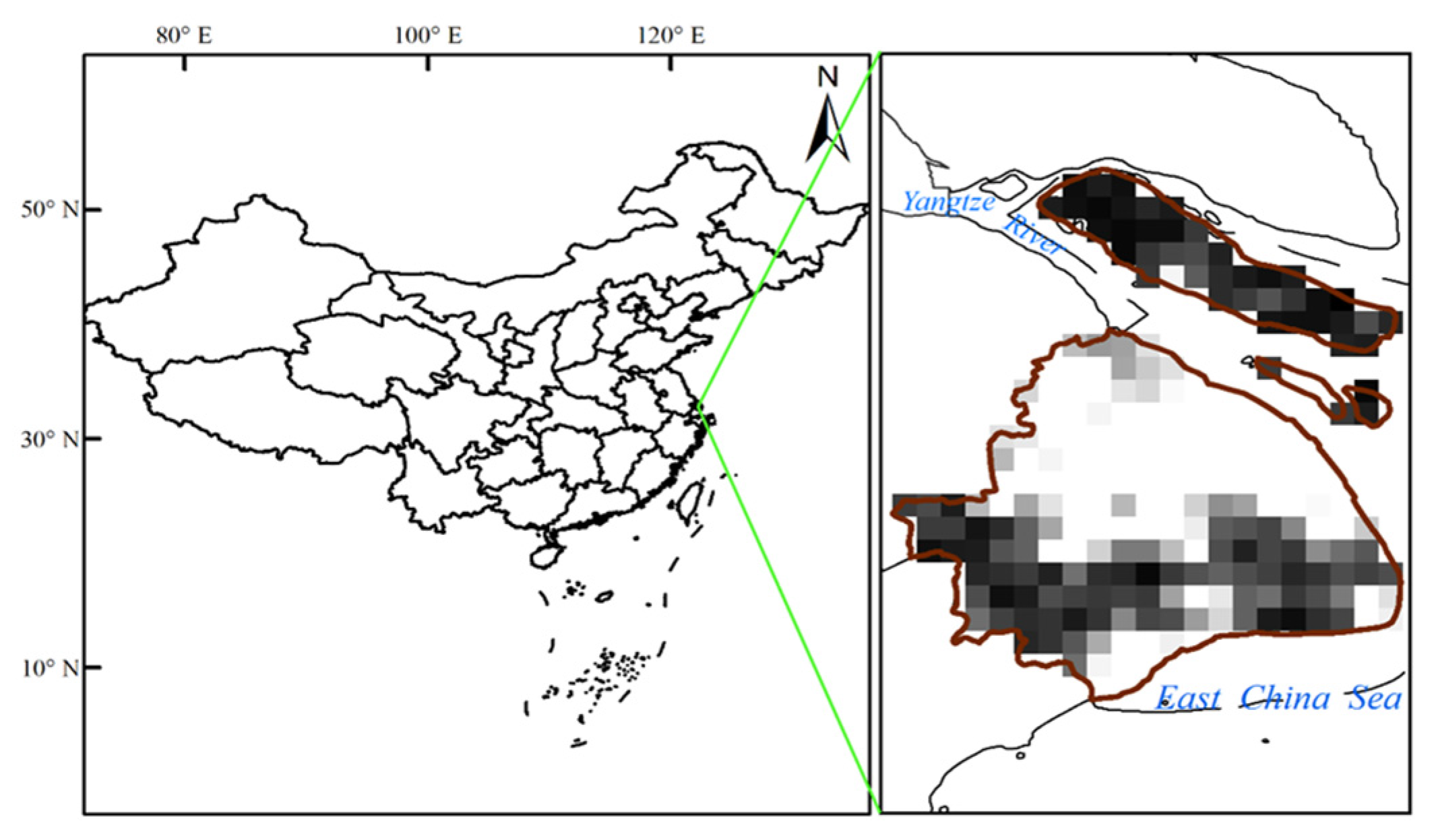
2.1. Study Area
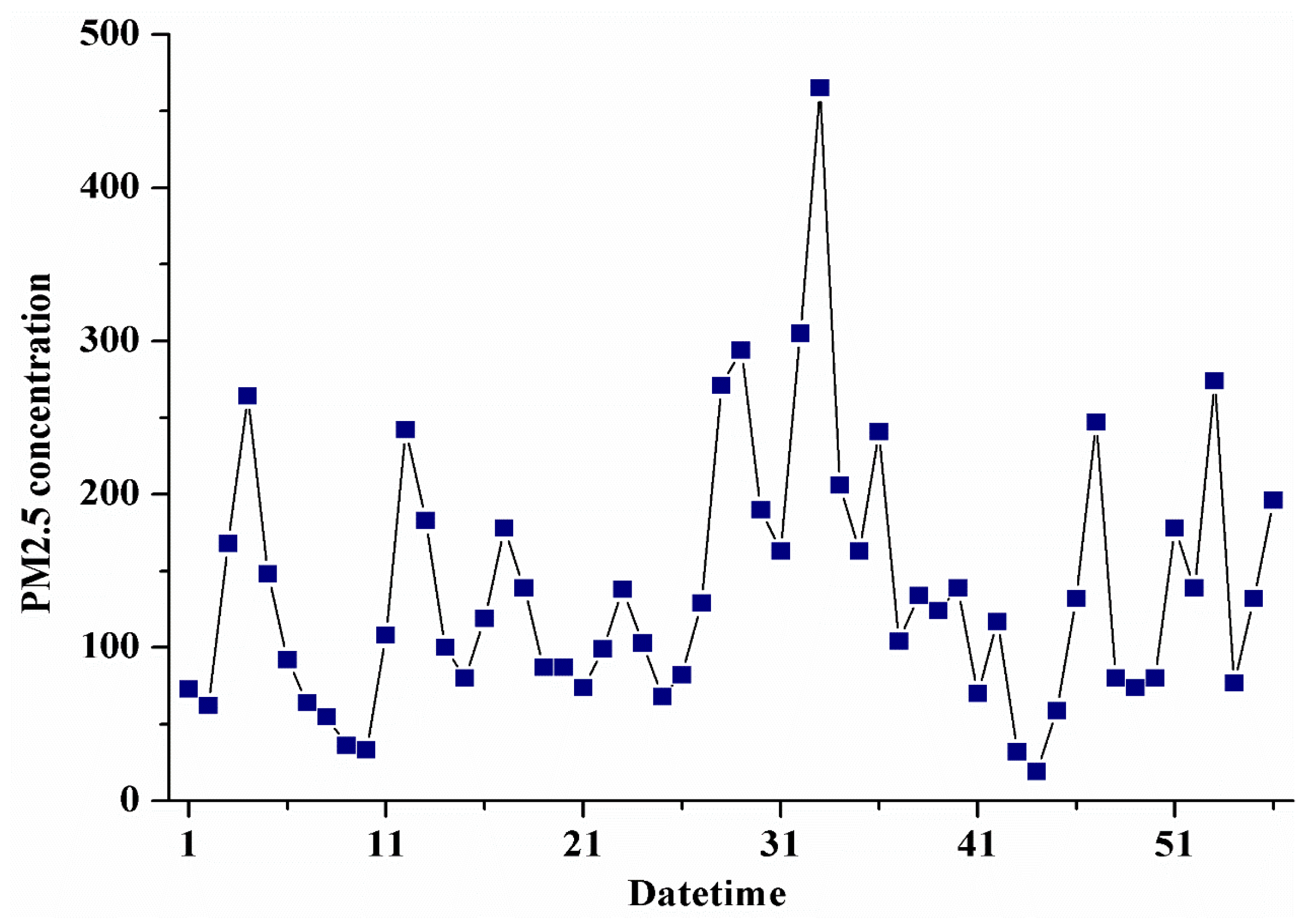
2.2. Data
3. Theory and Methods
3.1. Gaussian Fitting
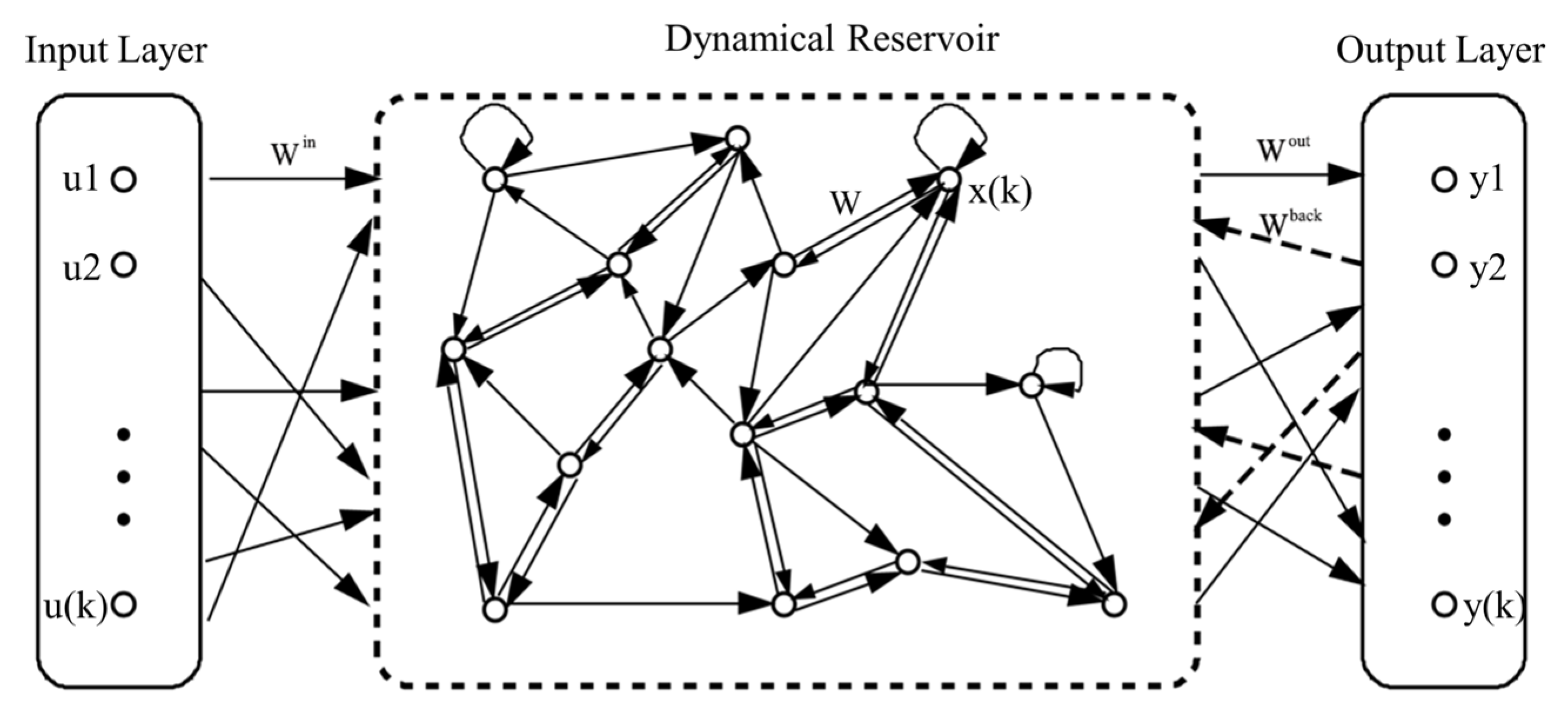
3.2. Echo State Networks
4. Results and Discussion
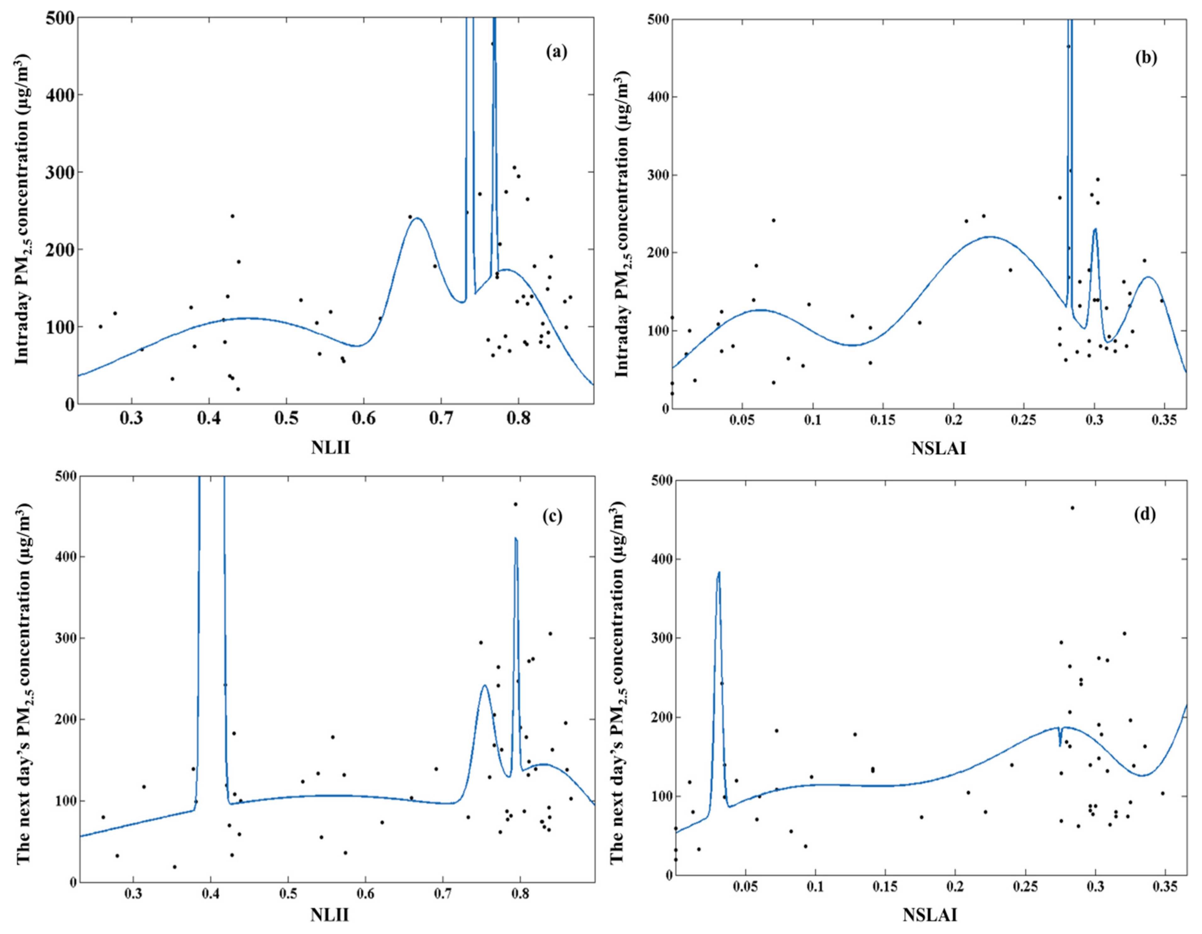
4.1. Relationship between Daily PM2.5 Average Concentrations and Nighttime Light Indices

| Fitting Coefficients | a | b | c | d |
|---|---|---|---|---|
| a1 | 595.600 | 9216.000 | 333.600 | −29.390 |
| b1 | 0.769 | 0.622 | 0.697 | 0.559 |
| c1 | 0.002 | 0.004 | 0.016 | 0.005 |
| a2 | 162.300 | 147.200 | 77.220 | −198.900 |
| b2 | 0.788 | 0.771 | 0.926 | 1.150 |
| c2 | 0.080 | 0.031 | 0.396 | 0.394 |
| a3 | 25360.000 | 219.900 | 135.800 | 313.000 |
| b3 | 0.737 | 0.153 | 0.476 | −1.476 |
| c3 | 0.002 | 0.618 | 0.091 | 0.026 |
| a4 | 109.800 | 124.500 | 118200.000 | 23080.000 |
| b4 | 0.450 | −1.222 | −1.414 | 11.620 |
| c4 | 0.208 | 0.538 | 0.036 | 5.092 |
| a5 | 185.700 | 147.200 | 106.200 | 63.180 |
| b5 | 0.667 | 1.100 | −0.573 | −1.097 |
| c5 | 0.040 | 0.183 | 2.192 | 0.722 |
| Goodness of Fitting | a | b | c | d |
|---|---|---|---|---|
| R2 | 0.2840 | 0.5096 | 0.5037 | 0.5126 |
| RMSE | 81.9732 | 68.0813 | 64.9732 | 62.6213 |
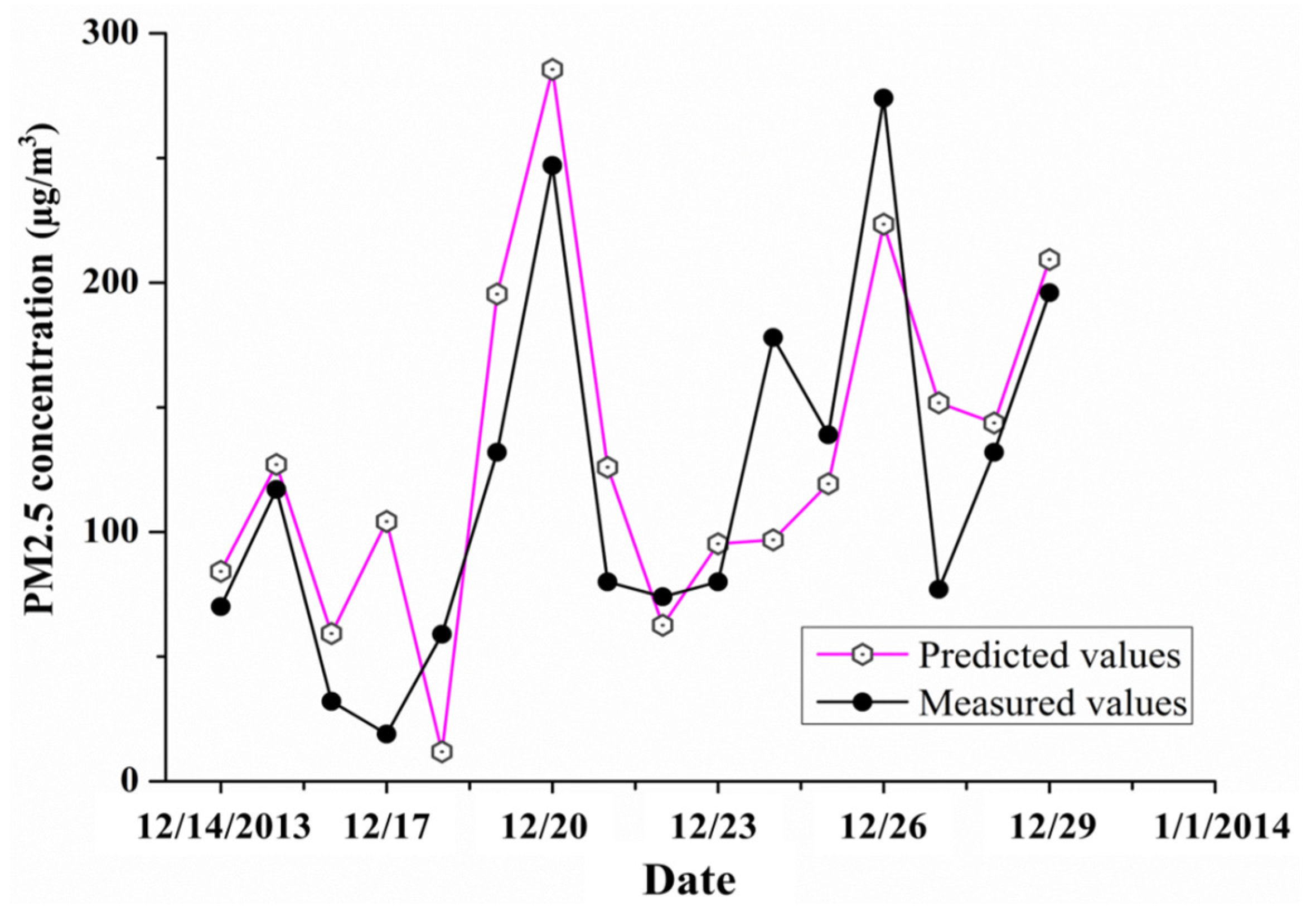
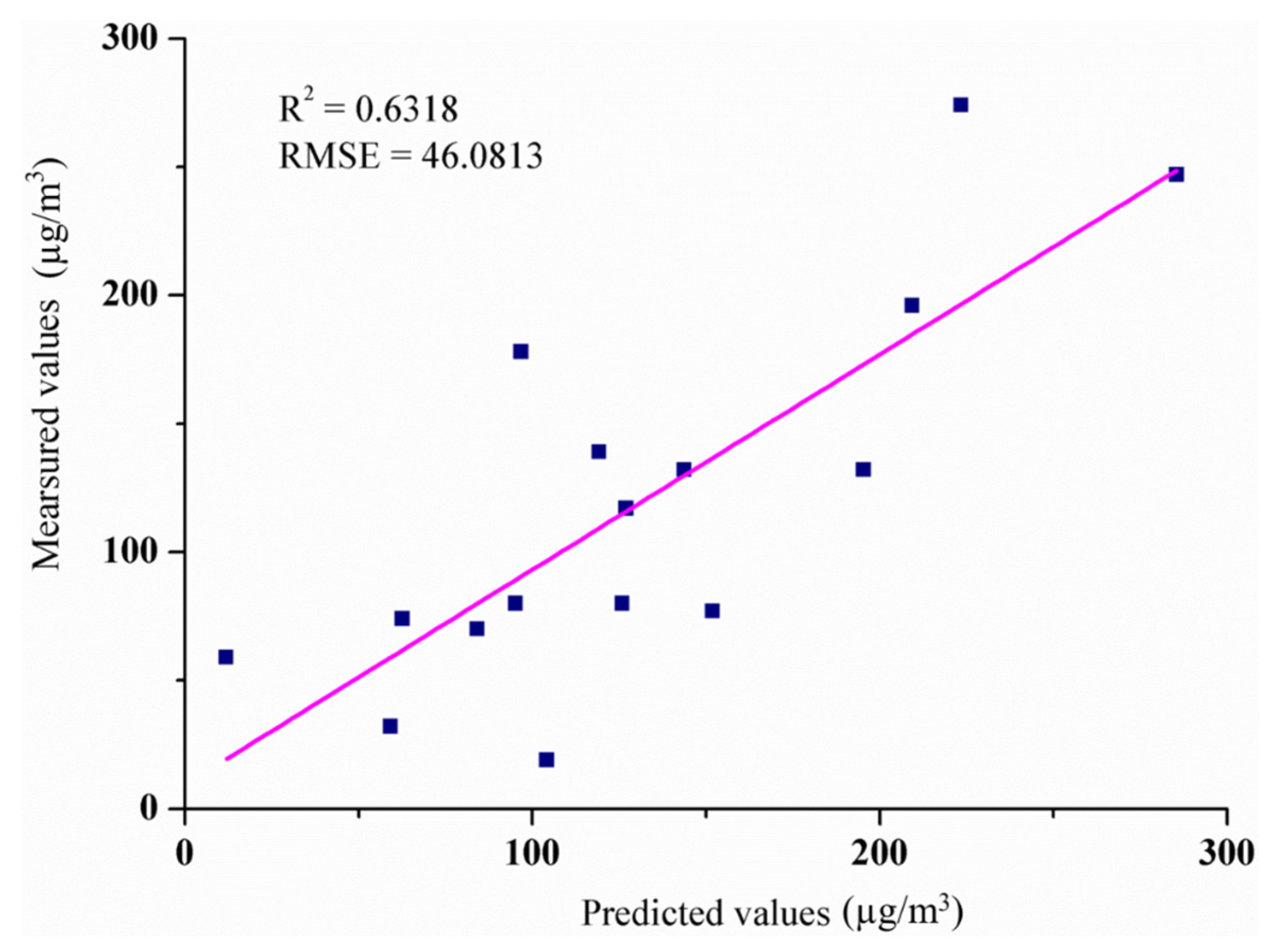
4.2. Verification of the Effectiveness of Nighttime Light Data that Used for the Prediction of Urban Daily PM2.5 Average Concentrations
5. Conclusions
Acknowledgments
Author Contributions
Conflicts of Interest
References
- Finlayson, B.J.; Pitts, J.N. Photochemistry of the polluted troposphere. Science 1976, 192, 111–119. [Google Scholar] [CrossRef] [PubMed]
- Bench, G.; Herckes, P. Measurement of contemporary and fossil carbon contents of PM2.5 aerosols: Results from Turtleback Dome, Yosemite National Park. Environ. Sci. Technol. 2004, 38, 2424–2427. [Google Scholar] [CrossRef] [PubMed]
- Fang, G.C.; Chang, C.N.; Wu, Y.S.; Fu, C.; Yang, D.G.; Chu, C.C. Characterization of chemical species in PM2.5 and PM10 aerosols in suburban and rural sites of central Taiwan. Sci. Total Environ. 1999, 234, 203–212. [Google Scholar] [CrossRef]
- Thomaidis, N.S.; Bakeas, E.B.; Siskos, P.A. Characterization of lead, cadmium, arsenic and nickel in PM2.5 particles in the Athens atmosphere, Greece. Chemosphere 2003, 52, 959–966. [Google Scholar] [CrossRef]
- Sun, W.; Zhang, H.; Palazoglu, A.; Singh, A.; Zhang, W.; Liu, S. Prediction of 24-hour-average PM2.5 concentrations using a hidden Markov model with different emission distributions in Northern California. Sci. Total Environ. 2013, 443, 93–103. [Google Scholar] [CrossRef] [PubMed]
- Fusco, A.C.; Logan, J.A. Analysis of 1970–1995 trends in tropospheric ozone at Northern Hemisphere midlatitudes with the GEOS-CHEM model. J. Geophys. Res.-Atmos. 2003, 108, D15. [Google Scholar] [CrossRef]
- Brasseur, G.P.; Hauglustaine, D.A.; Walters, S.; Rasch, P.J.; Muller, J.F.; Granier, C.; Tie, X.X. A global chemical transport model for ozone and related chemical tracers 1. Model description. J. Geophys. Res.-Atmos. 1998, 103, 28265–28289. [Google Scholar] [CrossRef]
- McKenna, D.S.; Grooss, J.U.; Gunther, G.; Konopka, P.; Muller, R.; Carver, G.; Sasano, Y. A new Chemical Lagrangian Model of the Stratosphere (CLaMS)-2. Formulation of chemistry scheme and initialization. J. Geophys. Res.-Atmos. 2002, 107, D15. [Google Scholar] [CrossRef]
- Saide, P.E.; Carmichael, G.R.; Spak, S.N.; Gallardo, L.; Osses, A.E.; Mena-Carrasco, M.A.; Pagowski, M. Forecasting urban PM10 and PM2.5 pollution episodes in very stable nocturnal conditions and complex terrain using WRF-Chem CO tracer model. Atmos. Environ. 2011, 45, 2769–2780. [Google Scholar] [CrossRef]
- Han, Z.; Ueda, H.; An, J. Evaluation and intercomparison of meteorological predictions by five MM5-PBL parameterizations in combination with three land-surface models. Atmos. Environ. 2008, 42, 233–249. [Google Scholar] [CrossRef]
- Manders, A.M.M.; Schaap, M.; Hoogerbrugge, R. Testing the capability of the chemistry transport model LOTOS-EUROS to forecast PM10 levels in the Netherlands. Atmos. Environ. 2009, 43, 4050–4059. [Google Scholar] [CrossRef]
- Cobourn, W.G. An enhanced PM2.5 air quality forecast model based on nonlinear regression and back-trajectory concentrations. Atmos. Environ. 2010, 44, 3015–3023. [Google Scholar] [CrossRef]
- Liu, Y.; Franklin, M.; Kahn, R.; Koutrakis, P. Using aerosol optical thickness to predict ground-level PM2.5 concentrations in the St. Louis area: A comparison between MISR and MODIS. Remote Sens. Environ. 2007, 107, 33–44. [Google Scholar] [CrossRef]
- Tao, J.; Zhang, M.; Chen, L.; Wang, Z.; Su, L.; Ge, C.; Han, X.; Zou, M. A method to estimate concentrations of surface-level particulate matter using satellite-based aerosol optical thickness. Sci. China-Earth Sci. 2013, 56, 1422–1433. [Google Scholar] [CrossRef]
- Lee, H.J.; Coull, B.A.; Bell, M.L.; Koutrakis, P. Use of satellite-based aerosol optical depth and spatial clustering to predict ambient PM2.5 concentrations. Environ. Res. 2012, 118, 8–15. [Google Scholar] [CrossRef] [PubMed]
- Li, X.; Chen, F.; Chen, X. Satellite-observed nighttime light variation as evidence for global armed conflicts. IEEE J. Sel. Top. Appl. Earth Obs. Remote Sens. 2013, 6, 2302–2315. [Google Scholar] [CrossRef]
- Jaeger, H.; Haas, H. Harnessing nonlinearity: Predicting chaotic systems and saving energy in wireless communication. Science 2004, 304, 78–80. [Google Scholar] [CrossRef] [PubMed]
- Manjunath, G.; Jaeger, H. Echo state property linked to an input: Exploring a fundamental characteristic of recurrent neural networks. Neural Comput. 2013, 25, 671–696. [Google Scholar] [PubMed]
- Feng, Y.; Chen, Y.; Guo, H.; Zhi, G.; Xiong, S.; Li, J.; Sheng, G.; Fu, J. Characteristics of organic and elemental carbon in PM2.5 samples in Shanghai, China. Atmos. Res. 2009, 92, 434–442. [Google Scholar] [CrossRef]
- NGDC. The National Geophysical Data Center. Available online: http://maps.ngdc.noaa.gov/viewers/index.html (accessed on 14 October 2015).
- The Shanghai Environment Monitoring Center. Available online: http://www.semc.com.cn/home/index.aspx (accessed on 14 October 2015).
- Yang, M.; Wang, S.; Zhou, Y.; Wang, L. Review on Application of DMSP/OLS nighttime Emissions Data. Remote Sens. Technol. Appl. 2011, 26, 45–51. [Google Scholar]
- Wang, H.; Zheng, X.; Yuan, T. Overview of Researches Based on DMSP/OLS Nighttime Light Data. Prog. Geogr. 2012, 31, 11–19. [Google Scholar]
- Xu, X. Physics for Remote Sensing; Peking University Press: Beijing, China, 2005. [Google Scholar]
- Liu, X.G.; Li, J.; Qu, Y.; Han, T.; Hou, L.; Gu, J.; Chen, C.; Yang, Y.; Liu, X.; Yang, T.; et al. Formation and evolution mechanism of regional haze: A case study in the megacity Beijing, China. Atmos. Chem. Phys. 2013, 13, 4501–4514. [Google Scholar] [CrossRef]
- Hu, J.; Wang, Y.; Ying, Q.; Zhang, H. Spatial and temporal variability of PM2.5 and PM10 over the North China Plain and the Yangtze River Delta, China. Atmos. Environ. 2014, 95, 598–609. [Google Scholar] [CrossRef]
- Kloog, I.; Chudnovsky, A.A.; Just, A.C.; Nordio, F.; Koutrakis, P.; Coull, B.A.; Lyapustin, A.; Wang, Y.; Schwartz, J. A new hybrid spatio-temporal model for estimating daily multi-year PM2.5 concentrations across northeastern USA using high resolution aerosol optical depth data. Atmos. Environ. 2014, 95, 581–590. [Google Scholar] [CrossRef]
- Wang, J.F.; Hu, M.G.; Xu, C.D.; Christakos, G.; Zhao, Y. Estimation of citywide air pollution in Beijing. PLoS ONE 2013, 8, e53400. [Google Scholar] [CrossRef] [PubMed]
- Feng, X.; Li, Q.; Zhu, Y.; Hou, J.; Jin, L.; Wang, J. Artificial neural networks forecasting of PM2.5 pollution using air mass trajectory based geographic model and wavelet transformation. Atmos. Environ. 2015, 107, 118–128. [Google Scholar] [CrossRef]
- Chen, J.; Zhuo, L.; Shi, P.J.; Toshiaki, I. The study on urbanization process in China based on DMSP/OLS data: Development of a light index for urbanization level estimation. J. Remote Sens. 2003, 7, 168–175. [Google Scholar]
- Axelsson, O. A generalized conjugate gradient, least square method. Numer. Math. 1987, 51, 209–227. [Google Scholar] [CrossRef]
- Kong, B.; Wang, Z.; Tan, Y. Gaussian fitting technique of laser spot. Laser Technol. 2002, 26, 277–278. [Google Scholar]
- Yildiz, I.B.; Jaeger, H.; Kiebel, S.J. Re-visiting the echo state property. Neural Netw. 2012, 35, 1–9. [Google Scholar] [CrossRef] [PubMed]
- Maass, W.; Natschläger, T.; Markram, H. Real-time computing without stable states: A new framework for neural computation based on perturbations. Neural Comput. 2002, 14, 2531–2560. [Google Scholar] [CrossRef] [PubMed]
- Jaeger, H. Short Term Memory in Echo State Networks; No. 152; National Research Center for Information Technology: Bremen: Germany, 2002. [Google Scholar]
- Pascanu, R.; Jaeger, H. A neurodynamical model for working memory. Neural Netw. 2011, 24, 199–207. [Google Scholar] [CrossRef] [PubMed]
- Xia, X.P. Prediction and space distribution analysis of PM2.5 daily average pollution levels based on ESN model in Beijing. Master’s Thesis, China University of Geosciences, Beijing, China, 2015. [Google Scholar]
- Ordieres, J.B.; Vergara, E.P.; Capuz, R.S.; Salazar, R.E. Neural network prediction model for fine particulate matter (PM2.5) on the US-Mexico border in El Paso (Texas) and Ciudad Judrez (Chihuahua). Environ. Model. Softw. 2005, 20, 547–559. [Google Scholar] [CrossRef]
© 2015 by the authors; licensee MDPI, Basel, Switzerland. This article is an open access article distributed under the terms and conditions of the Creative Commons Attribution license (http://creativecommons.org/licenses/by/4.0/).
Share and Cite
Xu, Z.; Xia, X.; Liu, X.; Qian, Z. Combining DMSP/OLS Nighttime Light with Echo State Network for Prediction of Daily PM2.5 Average Concentrations in Shanghai, China. Atmosphere 2015, 6, 1507-1520. https://doi.org/10.3390/atmos6101507
Xu Z, Xia X, Liu X, Qian Z. Combining DMSP/OLS Nighttime Light with Echo State Network for Prediction of Daily PM2.5 Average Concentrations in Shanghai, China. Atmosphere. 2015; 6(10):1507-1520. https://doi.org/10.3390/atmos6101507
Chicago/Turabian StyleXu, Zhao, Xiaopeng Xia, Xiangnan Liu, and Zhiguang Qian. 2015. "Combining DMSP/OLS Nighttime Light with Echo State Network for Prediction of Daily PM2.5 Average Concentrations in Shanghai, China" Atmosphere 6, no. 10: 1507-1520. https://doi.org/10.3390/atmos6101507
APA StyleXu, Z., Xia, X., Liu, X., & Qian, Z. (2015). Combining DMSP/OLS Nighttime Light with Echo State Network for Prediction of Daily PM2.5 Average Concentrations in Shanghai, China. Atmosphere, 6(10), 1507-1520. https://doi.org/10.3390/atmos6101507