Article

Combining DMSP/OLS Nighttime Light with Echo State Network for Prediction of Daily PM2.5 Average Concentrations in Shanghai, China

1
School of Information Engineering, China University of Geosciences, Beijing 100083, China
2
Qinhuangdao City Environmental Protection Bureau, Qinhuangdao 066000, China
*
Author to whom correspondence should be addressed.
Atmosphere 2015, 6(10), 1507-1520; https://doi.org/10.3390/atmos6101507
Submission received: 19 June 2015 / Revised: 28 September 2015 / Accepted: 13 October 2015 / Published: 19 October 2015

Abstract

:
The objective of this study is to investigate the potential of nighttime light data, acquired with Defense Meteorological Satellite Program Operational Linescan System (DMSP/OLS) owned by National Oceanic and Atmospheric Administration (NOAA), in predicting urban daily particulate matter (PM)2.5 with an aerodynamic diameter of less than 2.5 µm average concentrations. To achieve the purpose, we firstly extracted two night light indices, the Nighttime Light Intensity Index (NLII) and the Nighttime Saturated Light Area Index (NSLAI) from DMSP/OLS images. Through Gaussian fitting of the relationship between the indices and the daily PM2.5 concentrations data released by the government, we found that the intraday nighttime light indices were all more relevant with the PM2.5 average concentrations of the next day in Shanghai. Therefore, the 56 sets of data, the light indices were collected from 3 November 2013 to 28 December 2013, the daily PM2.5 concentrations data were collected from 4 November 2013 to 29 December 2013, and these were divided into two parts. The first 40 sets were used for training the model of echo state network (ESN). The last 16 sets were used for testing. The value of R2 of predicted results was as high as 0.6318. In summary, the effectiveness of nighttime light data that used for the prediction of urban daily PM2.5 average concentrations was verified in this study.

1. Introduction

Air quality issues are increasingly subject to public attention. Nitrogen oxide (NOx), carbon monoxide(CO), sulfur dioxide(SO2), as well as secondary pollutants such as ozone (O3) and particulate matter with an aerodynamic diameter of less than 2.5 µm (PM2.5) will have a direct or indirect impact on human health and plant growth [1,2]. Long-term exposure to PM2.5 will lead to the increase in the incidence of associated diseases (e.g., respiratory, cardiovascular disease, reduced lung function, heart attacks) in human beings [3,4]. Therefore, the real-time monitoring of PM2.5 concentrations and the prediction of its trend are particularly necessary.
However, the project merely establishing real-time monitoring stations to collect PM2.5 concentrations data would be complex, vast, costly and limited in terms of spatio-temporal coverage. Because PM2.5 concentrations in the air are affected by many potential-based instability factors, such as human activities and meteorological factors. Anthropogenic factors such as automobile exhaust, industrial discharges, fossil fuel combustion and coal burning are the main sources of PM2.5 concentrations. Meteorological factors include wind speed, wind direction, temperature, relative humidity, dew point and precipitation [5]. Fortunately, satellite derived data are an efficient important source and can help compensate for this limitation of monitoring stations.
Many studies have focused on the prediction of PM2.5 concentrations. Two types of methods (deterministic and statistical methods) are generally used. Deterministic methods are based on a chemical-transport model that includes GEOS-Chem [6], MOZART [7], CLaMS [8] and WRF-Chem [9]. These models are based on different chemical mechanism, chemical kinetics equation and a series of gas phase photochemical reaction, which would help to understand the physical mechanism, however, they also possess great application difficulties because of the large numbers of parameters for modeling. Their accuracy is limited by the scale they are applied and the quality of the emission data [10]. On account of the inherent complexity, low accuracy and computational intensiveness of deterministic methods, statistical methods are more appropriate for air quality forecasting [11,12].
Much satellite data and statistical methods were used in the study for forecasting PM2.5 concentrations. Using two general linear regression models, Liu et al. [13] compared the ability of the aerosol optical thickness (AOT) retrieved by the Multiangle Imaging SpectroRadiometer (MISR) and the Moderate Resolution Imaging Spectroradiometer (MODIS) to predict ground-level PM2.5 concentrations in St. Louis, MO and its surrounding areas [13]. MISR and MODIS have different instrument designs and retrieve aerosol optical properties using different algorithms. Surface-level particulate matter concentrations were estimated by using the data simulated by an atmospheric boundary layer model regional atmospheric modeling system (RAMS) and MODIS satellite-retrieved AOT in the study of Tao et al. [14]. Lee et al. [15] used satellite-based aerosol optical depth and spatial clustering for the prediction of ambient PM2.5 concentrations [15].
In this study, we firstly explored the relationship between nighttime light data and daily PM2.5 average concentrations in shanghai. Then, we employed echo state network (ESN) as statistic method to predict PM2.5 concentrations. Satellite data were used from the Defense Meteorological Satellite Program Operational Linescan System (DMSP/OLS) owned by National Oceanic and Atmospheric Administration (NOAA) in United States is a new choice for forecasting urban daily PM2.5 average concentrations. The DMSP satellites, with the onboard OLS, have the capability to detect faint sources of visible near-infrared (VNIR 400~1000 nm) emissions on the Earth’s surface, making it possible to detect cities and towns. This capability allows the mapping of urban night-time light emissions (upward light emissions) from terrestrial sources [16]. These night-time light radiation signal would been scattered by aerosol particles in the air such as PM2.5. Therefore, the radiation signal accepted by DMSP would been influenced by PM2.5 concentrations. Through the Gaussian fitting of the relationship between the daily PM2.5 concentrations data released by the government and the indices extracted from nighttime light data, we could concluded that there may be a functional relationship existed between them. ESN is a novel recurrent neural network (RNN) proposed by Jaeger and Haas (2004) [17]. Its basic idea is to use a large ‘‘reservoir” as a supplier of interesting dynamics from which the desired output is combined. The reservoir can remember the past history input and the memory will decay when time moves on [18]. This feature maybe coincides with our observation of urban daily PM2.5 average concentrations. In this paper, we also verified the effectiveness of using nighttime light data with ESN to predict the future urban PM2.5 average concentrations in a short-term.

2. Study Area and Data

2.1. Study Area
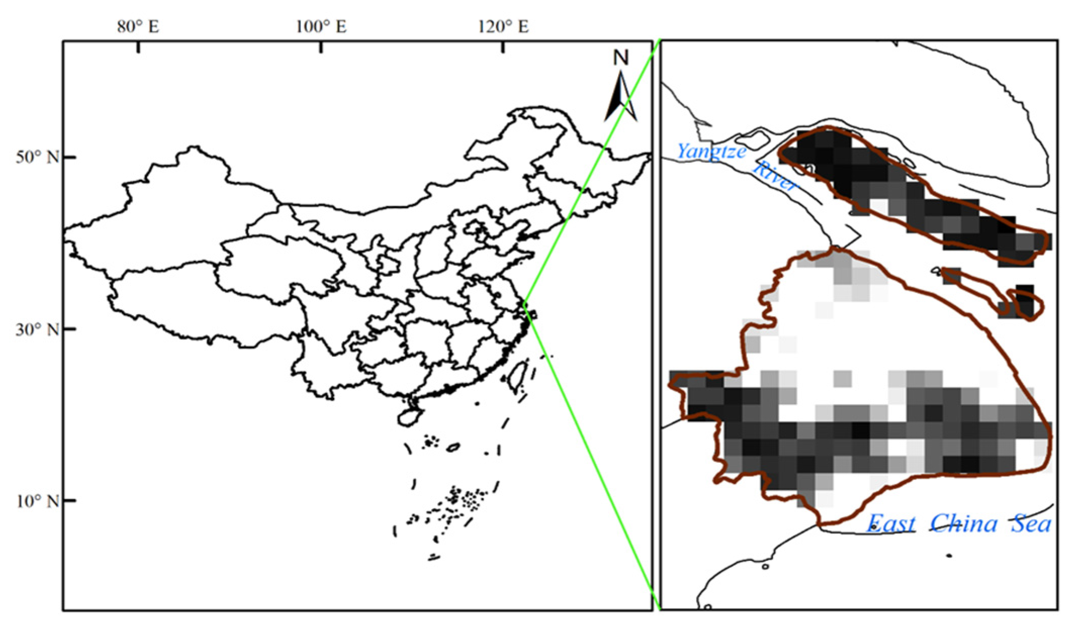
Shanghai is located at the east end of the Yangtze River Delta Region and faces the East China Sea (Figure 1), and possesses a population of over 15 million and a land area of about 6340 km2 [19]. Shanghai belongs to the northern subtropical monsoon climate, and northwest wind prevails in winter time whereas southeast wind in summertime. Annual average of temperature in Shanghai is 15.8 °C. Although some great efforts have been made by local governments for controlling the air pollution, such as the use of low-sulfur coal, the partial replacement of coal with liquefied petroleum gas or natural gas, the move-out of those highly polluted industry from the city and so on, the particulate matter sometimes still stays at a much higher level than the national air quality standard.
Figure 1. The location of study area and the trimmed nighttime light image of Shanghai, China.
Atmosphere 06 01507 g001

2.2. Data

The collected data consists of two parts. One part is nighttime light images. The other part is daily average PM2.5 concentrations data.
Visible nighttime imageries from DMSP/OLS instruments were collected from the website of National Geophysical Data Center [20] from 3 November 2013 to 28 December 2013. The continuous analog signal is sampled at a constant rate so the Earth-located centers of each pixel are roughly equidistant, i.e., 0.5 km apart [16]. Then nighttime light imageries of Shanghai could be obtained by the clipping based on the vector of Shanghai’s administrative boundary.
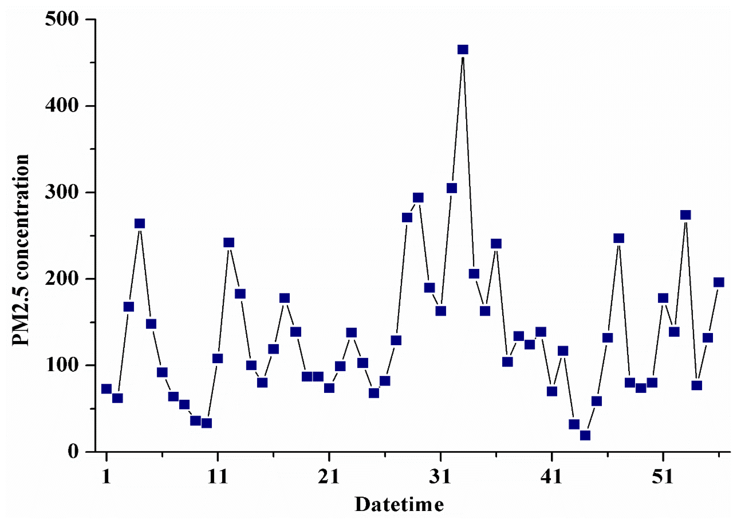
Daily average PM2.5 concentrations from 3 November 2013 to 29 December 2013 were collected from the website of Shanghai Environment Monitoring Center [21]. The time series data has 57 points. Figure 2 shows the daily average concentrations of PM2.5 during the period.
Figure 2. Daily average concentrations of PM2.5 in Shanghai from 3 November 2013 to 29 December 2013. Unit is μg·m−3.
Atmosphere 06 01507 g002

3. Theory and Methods

In general, OLS visible data record visible and near-Infrared emissions from the sun or the moon reflected off clouds and other features. Ground-based sources such as fires and upper atmospheric sources like the northern lights are seen [22,23]. For the city like Shanghai, nighttime light data mainly collected radiation signal of the lamplight, the fire and so on. However, according to Wave Equation, these radiation signals would be scattered by aerosol particles such as PM2.5 [24]. Meanwhile, PM2.5 was relatively concentrated in developed countries such as the USA, Australia, and some European countries and most major cities in China, especially for Beijing, Tianjin and Shanghai, known as a rapidly developed agglomeration [25,26,27,28,29]. Therefore, the PM2.5 concentration of the city is one of the influence factors of nighttime light data. The nighttime light data may also reflect the feature of the PM2.5 concentrations. In order to validate the correlation between the PM2.5 concentrations and nighttime light data, two night light indices, the Nighttime Light Intensity Index (NLII) and the Nighttime Saturated Light Area Index (NSLAI) were extracted from DMSP/OLS imagery based on Chen et al.’s study [30]. The two light indices that could represent the feature of nighttime light data: NLII characterized the ratio of effective light intensity to maximum light intensity and NSLAI characterized the ratio of area of saturated light pixels to total area of Shanghai, China. If it was not affected by PM2.5, the nighttime light of the major city is relatively saturated.
N L I I = i = 1 63 D N i × n i N × 63
N S L A I = A r e a 63 A r e a a l l
In Equations (1) and (2), there were totally five variables as follows. DNi: DN value which equals to i; ni: Number of pixels whose DN values equal to i; N: Number of effective lighting pixels, whose DN values range from 1 to 63; Area63: Area of saturated light pixels which DN value equals to 63; Areaall: Total area of all pixels of Shanghai.
Then, through fitting, we could conclude that whether or not functional relationship exists between the nighttime light indices and PM2.5 concentrations. The Gaussian Fitting method was employed to compute the correlation between the two light indices and the intraday PM2.5 concentrations respectively. Intraday means a whole day from 0 to 24. In this paper, the correlation between the two intraday light indices and the PM2.5 concentrations of the next day as well as intraday was computed. The reason is that the intraday nighttime light imagery was gained at night which may impact on the PM2.5 concentrations of the next day. Through comparison, the better correlation should be gotten.

3.1. Gaussian Fitting

Gaussian function has peak characteristics. In addition, the relations, in this paper, between PM2.5 and the two light indices have multi-peak characteristics, so a combination of multiple Gaussian function was used to fit the correlation between intraday nighttime light indices (NLII, NSLAI) and the intraday PM2.5 concentrations data (or the PM2.5 concentrations of the next day) and the Gaussian Fitting method was applied to compute the goodness of fit respectively.
For example, sample sequences were (NLII1, PM1), (NLII2, PM2), (NLII3, PM3) … (NLIIn, PMn). Taking Gauss base equation:
y = a 1 e x p ( ( ( x b 1 ) / c 1 ) 2 )
In this equation, a1, b1 and c1 all are the undetermined coefficients.
After taking natural logarithms available for each side of Equation (3):
Y = A x 2 + B x + C
In Equation (4), there were totally four variables as follows.
{ Y = ln ( y ) A = 1 / c 1 2 B = 2 b 1 / c 1 2 C = b 1 2 / c 1 2 ln ( a 1 )
According to the principle of least square method [31], the undetermined parameters of Equation (3) could be solved [32].
{ a 1 = e x p ( B 2 / 4 A C ) b 1 = B / 2 A c 1 = 1 / A
In this study, General model Gauss5 was used for the fitting. Gauss5 model means the combination of five Gaussian base Equations like Equation (3). The Gauss5 function is given like this:
f ( x ) = i = 1 5 a i e x p ( ( ( x b i ) / c i ) 2 )
Duo to the kernel of Gauss5 is based on Gaussian base Equation, so Gauss5 could also be figured out based on least square method. Then, the fifteen undetermined coefficients (a1, b1, c1 … a5, b5, c5) would also been solved with 95% confidence bounds. The performance of each fitting was investigated with three parameters: the correlation coefficient (R2) and root mean square errors (RMSE).
The two parameters were calculated by:
R 2 = [ i = 1 N ( y a i y a ¯ ) i = 1 N ( y m i y m ¯ ) ] 2 i = 1 N ( y a i y a ¯ ) 2 i = 1 N ( y m i y m ¯ ) 2
R M S E = 1 N 1 i = 1 N ( y a i y m i ) 2
In the above two parameters, R2 was calculated to analyze the accuracy of fitting values versus measured values. R2 value range from 0 to 1. The higher the R2 value is, the stronger indication of an existing correlation between the fitting and measured values. Meanwhile, the lower the RMSE value is, the stronger indication of small estimation errors.

3.2. Echo State Networks

After Gaussian Fitting, the correlation between nighttime light indices and daily PM2.5 concentrations would be obtained. However, the fitting accuracy is relatively low. Duo to the feature of time series dynamic and nonlinearity that existed in light indices and PM2.5 concentrations data, Echo state networks (ESN) was employed to predict the PM2.5 concentrations based on the nighttime light indices. In previous studies, ESN not only has a unique network structure, strong characteristics of short-term memory but also use linear regression equation to train weights. Therefore, it could greatly simplify the neural network training. At the same time, it makes sure that these weights are global optimal solution and has good generalization ability. In addition, it avoids the complex situation in common neural network training and local optimum. Compared with the traditional artificial neural network (ANN), ESN has higher efficiency training, faster training speed and more stable, etc. [33,34,35].
ESN provide an architecture and supervised learning principle for recurrent neural networks (RNNs) [33]. The main idea is (1) to drive a random, large, fixed recurrent neural network with the input signal, thereby inducing in each neuron within this “reservoir” network a nonlinear response signal, and (2) combine a desired output signal by a trainable linear combination of all of these response signals. The basic idea of ESNs is shared with Liquid State Machines (LSM), which were discovered and investigated independently from and simultaneously with ESNs by Wolfgang Maass [34,35].
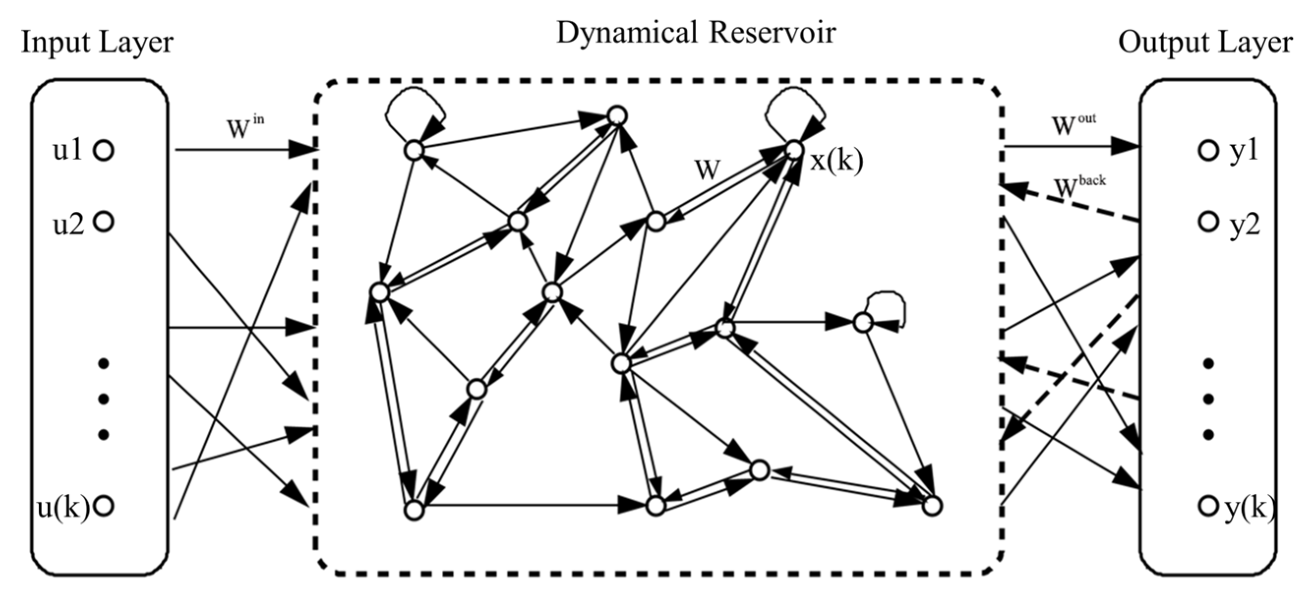
Figure 3. The architecture of an echo state network.
Atmosphere 06 01507 g003
A standard ESN consists of three layers with K units in the input layer, N nodes in the internal (hidden) layer and L units in the output layer. The network architecture of ESN is shown in Figure 3. All K input nodes are connected to all N internal units and all N internal units are connected to the L nodes in the output layer. Additionally, the output neurons can be fed back to the internal layer. Compared with other conventional neural networks, ESN often has a larger number of neurons (on the order of 50–1000) in the internal layer, which are sparsely interconnected. Note that connections directly from the input to the output units and connections between output units are allowed. In order to have echo states, the magnitude of the largest eigenvalue of the internal connection weight matrix must satisfy |λmax| < 1. In fact, the reservoir itself is fixed, once it is chosen. Moreover, during the training process of ESN, only the output connections are changed through offline linear regression or online methods [36].
The update equation and readout layer equation are defined as:
x ( k + 1 ) = f ( W i n u ( k + 1 ) + W x ( k ) + W b a c k y ( k ) )
y ( k + 1 ) = f o u t ( W o u t ( u ( k + 1 ) , x ( k + 1 ) ) )
where u (k) is a known input variable, x (k) is a vector of reservoir neuron activations and y (k) is the output variable, all at time step k. The Win, W and Wback are the input weight matrices, recurrent weight matrices and feedback weight matrices connections from the output to the reservoir. Function f is the activation function of reservoir and applied element-wise. And the tanh (sigmoidal function) function is the most common choice be used as the function f. where function fout can be either linear or sigmoidal, depending on the complexity of the task. In this study, sigmoidal function was used as fout. The Wout denotes the weight matrix of output connections, which is determined through network training.
Assuming that there are M samples {μ (i), y (i)}, i = 1,2,…,m, ESN approach is learned by the following steps.
(1) Initializing the ESN. It would generate three random matrices (Win, W, Wback).
(2) Running it using the training input u (i) and collect the corresponding reservoir activation states x (i).
(3) Computing the readout weights matrix Wout from the reservoir using direct pseudoinverse solution.
W o u t = Y X +
where X = (x (n+1), x (n+2), …, x (m))T, Y = (y (n+1),y (n+2), …, y (m))T, n is the initial step. X+ is the Moore-Penrose pseudoinverse of X.
(4) Using the trained network on new input data u (n) computing y (n) by employing the trained readout weights matrix Wout.
The performance of prediction was also investigated with two parameters: the correlation coefficient (R2) and the root mean square errors (RMSE) that can be seen at Equations (8) and (9).

4. Results and Discussion

The first goal of this study is to validate the correlation between the intraday nighttime light indices and daily PM2.5 concentrations. The second goal is to find out the better correlation between the nighttime light indices and intraday PM2.5 concentrations (or the next day’s PM2.5 concentrations). According to the previous two goals, the third goal of this study is using nighttime light data for prediction of daily PM2.5 concentrations based on ESN method. This is the process from validation to application.

4.1. Relationship between Daily PM2.5 Average Concentrations and Nighttime Light Indices
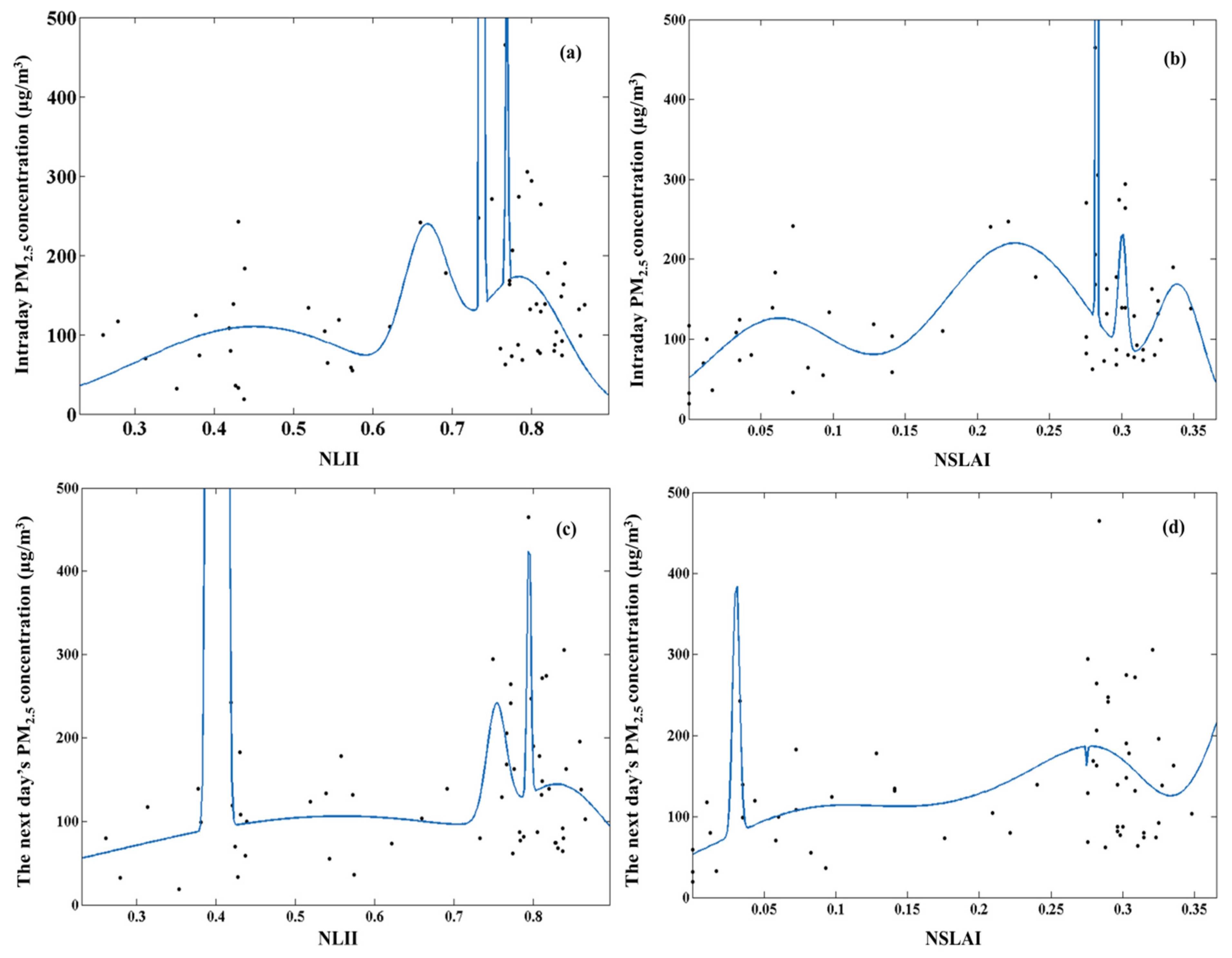
Figure 4 shows the Gaussian Fitting results between nighttime light indices and daily PM2.5 concentrations in Shanghai. Table 1 shows the values of the fifteen coefficient of Gauss5 of each fitting results. From these four figures, we can find out that there is no obvious high correlation between nighttime light indices and daily PM2.5 concentrations neither the intraday nor the next day. However, there are some subtle multi-peak features between the daily PM2.5 average concentrations and nighttime light indices existed in these figures, which is the reason why we use Gaussian Fitting and the number of terms is as high as five. Table 2 shows the performance of fitting. The values of R2 of each fitting figure is larger than 0, which means there is certain correlation between nighttime light indices and daily PM2.5 concentrations in Shanghai. The first goal of this study has been achieved. However, the value of R2 of the fitting between intraday NLII and intraday PM2.5 concentrations is equal to 0.2840, which is smaller than the value of R2 of the fitting between intraday NLII and the next day’s PM2.5 concentrations that is equal to 0.5096. Also, the value of RMSE of the fitting between intraday NLII and intraday PM2.5 concentrations is equal to 81.9732, which is larger than the value of RMSE of the fitting between intraday NLII and the next day’s PM2.5 concentrations that is equal to 68.0813. Likewise, for the other light index NSLAI, the value of R2 of the fitting between it and intraday PM2.5 concentrations is equal to 0.5037, which is smaller than the value of R2 of the fitting between it and the next day’s PM2.5 concentrations that is equal to 0.5126. The value of RMSE of the fitting between intraday NSLAI and intraday PM2.5 concentrations is equal to 64.9732, which is larger than the value of RMSE of the fitting between intraday NSLAI and the next day’s PM2.5 concentrations that is equal to 62.6213. To sum up, no matter NLII or NSLAI, the goodness of fitting between the nighttime light indices and the next day’s PM2.5 concentrations was better than intraday. Therefore, it may conclude that the intraday nighttime light indices were all more relevant with the PM2.5 concentrations of the next day in Shanghai. Hence, the second goal of this study has been achieved.
Figure 4. Gaussian fitting between the daily PM2.5 concentrations and nighttime light indices. (a) NLII vs. intraday PM2.5 concentrations; (b) NSLAI vs. intraday PM2.5 concentrations; (c) NLII vs. the next day’s PM2.5 concentrations; (d) NSLAI vs. the next day’s PM2.5 concentrations.
Atmosphere 06 01507 g004
Table 1. The fifteen coefficients of Gauss5 equations of the four Gaussian fitting combinations.
Fitting Coefficientsabcd
a1595.6009216.000333.600−29.390
b10.7690.6220.6970.559
c10.0020.0040.0160.005
a2162.300147.20077.220−198.900
b20.7880.7710.9261.150
c20.0800.0310.3960.394
a325360.000219.900135.800313.000
b30.7370.1530.476−1.476
c30.0020.6180.0910.026
a4109.800124.500118200.00023080.000
b40.450−1.222−1.41411.620
c40.2080.5380.0365.092
a5185.700147.200106.20063.180
b50.6671.100−0.573−1.097
c50.0400.1832.1920.722
Table 2. The performance of Gaussian fitting of the four fitting combinations.
Goodness of Fittingabcd
R20.28400.50960.50370.5126
RMSE81.973268.081364.973262.6213

4.2. Verification of the Effectiveness of Nighttime Light Data that Used for the Prediction of Urban Daily PM2.5 Average Concentrations
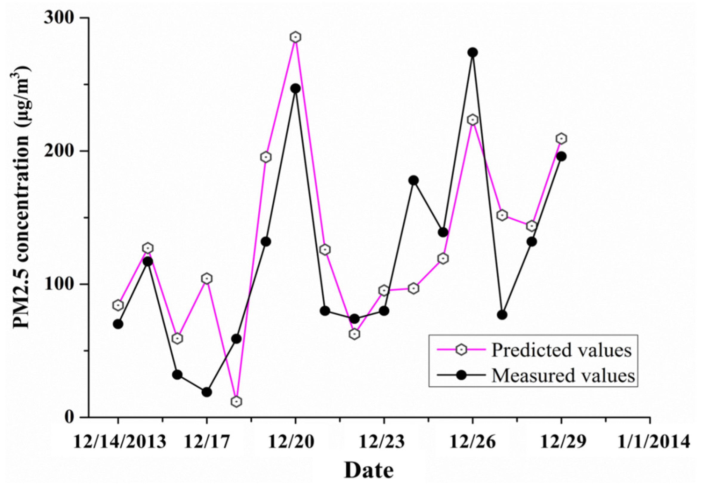
According to the achieved first and second goal, we could conclude that there may exist a certain functional relationship between the nighttime light indices (NLII and NSLAI) and the next day’s PM2.5 concentrations in Shanghai. Then, the intraday nighttime light indices (NLII and NSLAI) were used as input variables of the ESN, the daily PM2.5 concentrations data was used as output target variables of the ESN, which means the dimension of input variables was equal to 2, the dimension of output variable was equal to 1. In this study, there are 56 sets of data in total. The foregoing continuous 40 sets of data were used as training data sets that involves both input light indices data and teacher-forcing the desired output daily PM2.5 concentrations data. And the last continuous 16 sets of data were used as testing data sets. Through training of the network, the readout weights matrix Wout would be figured out. The trial method in this paper was used to find a proper size of the dynamical reservoir from 50 to 1000 with 50 as step length. With the size of the dynamical reservoir we could produce random sparse matrix as the dynamical reservoir for ESN to initialize the ESN [37]. Once the readout weights matrix Wout was obtained, the predicted value of daily PM2.5 concentrations would been calculated based on the update equation and readout layer equation of the echo state network. The predicted results and testing values of daily PM2.5 concentrations are shown in Figure 5. For clarity, we also need to compare the 16 predicted values and testing measured values of daily PM2.5 concentrations, and evaluate the prediction effect of ESN. From Figure 5, we could find that the overall trend of the predicted results is similar to the trend of measured values of daily PM2.5 concentrations in Shanghai. However, there were some days’ prediction errors of daily PM2.5 concentrations is large, such as 17 December 2013, 24 December 2013, 27 December 2013. In addition to the instantaneous feature of nighttime light imagery, the prediction errors may be mainly caused by the weather in the next day’s daytime that would impact on the PM2.5 concentrations distribution and made the functional correlation between the intraday nighttime light indices and the next day’s PM2.5 concentrations weaker.
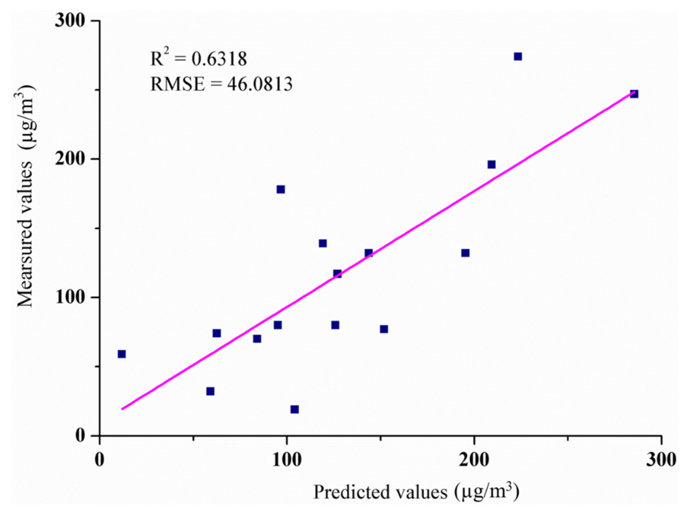
The accuracy evaluation of predicted result is shown in Figure 6. The value of R2 of predicted results was as high as 0.6318. Additionally, the value of RMSE was equal to 43.5259. In contrast, Ordieres et al. [38] used three types of ANNs to predict daily average PM2.5 at El Paso (Texas) and Ciudad Juárez (Chihuahua) and found that radial basis function ANN (RBF-ANN) had the shortest training time and a greater stability during prediction stage [36]. In their work, average levels of PM2.5 during the first 8h of the day, maximum level of PM2.5 of the first 8h of the day, temperature, relative humidity, wind speed, and wind directions were selected as input variables. The highest correlation factor (R2) was 0.4611 and the average error was about 30%. In comparison with the results of the work of Ordieres et al. [38], we used lesser input variables and had higher prediction accuracy, which means we would achieve better prediction effect based on lesser input data. The relative high prediction accuracy maybe means the nighttime light data could be used for prediction of daily PM2.5 concentrations in city, which will create a new path for daily PM2.5 concentrations prediction in city.
Figure 5. The comparison between the predicted values and measured values of daily PM2.5 concentrations within 16 days.
Atmosphere 06 01507 g005
Figure 6. The accuracy of the predicted values relative to the measured values of daily PM2.5 average concentrations.
Atmosphere 06 01507 g006

5. Conclusions

Remote sensing has the capacity to detect conditions of earth surface and atmosphere, thus it has some potential to find land changes influenced by PM2.5 concentrations. Remote sensing has been widely applied for predicting PM2.5 concentrations. However, only a few studies have used nighttime light data to inversed PM2.5 concentrations. In this article, the DMSP/OLS nighttime light images, with high temporal resolution and low price, were found can be used for urban daily PM2.5 average concentrations. Through the Gaussian fitting of the relationship between the daily PM2.5 concentrations data released by the government and the indices extracted from nighttime light data, we could conclude that there may be a functional relationship existing between them. In addition, we found that the intraday nighttime light indices were all more relevant with the PM2.5 average concentrations of the next day in Shanghai. The accuracy of predicted result is reliable. It can be inferred that the nighttime light data applied in daily PM2.5 average concentrations forecasting in short-term has some research significance and values.
This study is a primary work on the effectiveness of nighttime light data that is used for the prediction of urban daily PM2.5 average concentrations, and more efforts should be invested in future work. For instance, more auxiliary data about weather will help to improve the accuracy of the predicted results. Moreover, the nighttime light data caused by natural disasters, which can also cause sharp change in nighttime lights, should also be investigated quantitatively.

Acknowledgments

The authors would like to thank the mates from the remote sensing laboratory of China University of Geosciences for their insightful comments that helped us to refine the conceptual aspects of the subject and hence enabled us to improve the performance on this work. We also want to acknowledge the help provided by Herbert Jaeger and Mantas Lukosevicius from Jacobs University. The authors wish to thank the anonymous reviewers for their constructive comments that helped improve the scholarly quality of the paper.

Author Contributions

Zhao Xu and Xiangnan Liu conceived and supervised the research topic. Zhao Xu and Xiaopeng Xia proposed the methods and processed the data. Zhao Xu analyzed the results and wrote the paper. Zhiguang Qian contributed to the editing and review of the manuscript. All authors read and approved the submitted manuscript, agreed to be listed and accepted the version for publication.

Conflicts of Interest

The authors declare no conflict of interest.

References

  1. Finlayson, B.J.; Pitts, J.N. Photochemistry of the polluted troposphere. Science 1976, 192, 111–119. [Google Scholar] [CrossRef] [PubMed]
  2. Bench, G.; Herckes, P. Measurement of contemporary and fossil carbon contents of PM2.5 aerosols: Results from Turtleback Dome, Yosemite National Park. Environ. Sci. Technol. 2004, 38, 2424–2427. [Google Scholar] [CrossRef] [PubMed]
  3. Fang, G.C.; Chang, C.N.; Wu, Y.S.; Fu, C.; Yang, D.G.; Chu, C.C. Characterization of chemical species in PM2.5 and PM10 aerosols in suburban and rural sites of central Taiwan. Sci. Total Environ. 1999, 234, 203–212. [Google Scholar] [CrossRef]
  4. Thomaidis, N.S.; Bakeas, E.B.; Siskos, P.A. Characterization of lead, cadmium, arsenic and nickel in PM2.5 particles in the Athens atmosphere, Greece. Chemosphere 2003, 52, 959–966. [Google Scholar] [CrossRef]
  5. Sun, W.; Zhang, H.; Palazoglu, A.; Singh, A.; Zhang, W.; Liu, S. Prediction of 24-hour-average PM2.5 concentrations using a hidden Markov model with different emission distributions in Northern California. Sci. Total Environ. 2013, 443, 93–103. [Google Scholar] [CrossRef] [PubMed]
  6. Fusco, A.C.; Logan, J.A. Analysis of 1970–1995 trends in tropospheric ozone at Northern Hemisphere midlatitudes with the GEOS-CHEM model. J. Geophys. Res.-Atmos. 2003, 108, D15. [Google Scholar] [CrossRef]
  7. Brasseur, G.P.; Hauglustaine, D.A.; Walters, S.; Rasch, P.J.; Muller, J.F.; Granier, C.; Tie, X.X. A global chemical transport model for ozone and related chemical tracers 1. Model description. J. Geophys. Res.-Atmos. 1998, 103, 28265–28289. [Google Scholar] [CrossRef]
  8. McKenna, D.S.; Grooss, J.U.; Gunther, G.; Konopka, P.; Muller, R.; Carver, G.; Sasano, Y. A new Chemical Lagrangian Model of the Stratosphere (CLaMS)-2. Formulation of chemistry scheme and initialization. J. Geophys. Res.-Atmos. 2002, 107, D15. [Google Scholar] [CrossRef]
  9. Saide, P.E.; Carmichael, G.R.; Spak, S.N.; Gallardo, L.; Osses, A.E.; Mena-Carrasco, M.A.; Pagowski, M. Forecasting urban PM10 and PM2.5 pollution episodes in very stable nocturnal conditions and complex terrain using WRF-Chem CO tracer model. Atmos. Environ. 2011, 45, 2769–2780. [Google Scholar] [CrossRef]
  10. Han, Z.; Ueda, H.; An, J. Evaluation and intercomparison of meteorological predictions by five MM5-PBL parameterizations in combination with three land-surface models. Atmos. Environ. 2008, 42, 233–249. [Google Scholar] [CrossRef]
  11. Manders, A.M.M.; Schaap, M.; Hoogerbrugge, R. Testing the capability of the chemistry transport model LOTOS-EUROS to forecast PM10 levels in the Netherlands. Atmos. Environ. 2009, 43, 4050–4059. [Google Scholar] [CrossRef]
  12. Cobourn, W.G. An enhanced PM2.5 air quality forecast model based on nonlinear regression and back-trajectory concentrations. Atmos. Environ. 2010, 44, 3015–3023. [Google Scholar] [CrossRef]
  13. Liu, Y.; Franklin, M.; Kahn, R.; Koutrakis, P. Using aerosol optical thickness to predict ground-level PM2.5 concentrations in the St. Louis area: A comparison between MISR and MODIS. Remote Sens. Environ. 2007, 107, 33–44. [Google Scholar] [CrossRef]
  14. Tao, J.; Zhang, M.; Chen, L.; Wang, Z.; Su, L.; Ge, C.; Han, X.; Zou, M. A method to estimate concentrations of surface-level particulate matter using satellite-based aerosol optical thickness. Sci. China-Earth Sci. 2013, 56, 1422–1433. [Google Scholar] [CrossRef]
  15. Lee, H.J.; Coull, B.A.; Bell, M.L.; Koutrakis, P. Use of satellite-based aerosol optical depth and spatial clustering to predict ambient PM2.5 concentrations. Environ. Res. 2012, 118, 8–15. [Google Scholar] [CrossRef] [PubMed]
  16. Li, X.; Chen, F.; Chen, X. Satellite-observed nighttime light variation as evidence for global armed conflicts. IEEE J. Sel. Top. Appl. Earth Obs. Remote Sens. 2013, 6, 2302–2315. [Google Scholar] [CrossRef]
  17. Jaeger, H.; Haas, H. Harnessing nonlinearity: Predicting chaotic systems and saving energy in wireless communication. Science 2004, 304, 78–80. [Google Scholar] [CrossRef] [PubMed]
  18. Manjunath, G.; Jaeger, H. Echo state property linked to an input: Exploring a fundamental characteristic of recurrent neural networks. Neural Comput. 2013, 25, 671–696. [Google Scholar] [PubMed]
  19. Feng, Y.; Chen, Y.; Guo, H.; Zhi, G.; Xiong, S.; Li, J.; Sheng, G.; Fu, J. Characteristics of organic and elemental carbon in PM2.5 samples in Shanghai, China. Atmos. Res. 2009, 92, 434–442. [Google Scholar] [CrossRef]
  20. NGDC. The National Geophysical Data Center. Available online: http://maps.ngdc.noaa.gov/viewers/index.html (accessed on 14 October 2015).
  21. The Shanghai Environment Monitoring Center. Available online: http://www.semc.com.cn/home/index.aspx (accessed on 14 October 2015).
  22. Yang, M.; Wang, S.; Zhou, Y.; Wang, L. Review on Application of DMSP/OLS nighttime Emissions Data. Remote Sens. Technol. Appl. 2011, 26, 45–51. [Google Scholar]
  23. Wang, H.; Zheng, X.; Yuan, T. Overview of Researches Based on DMSP/OLS Nighttime Light Data. Prog. Geogr. 2012, 31, 11–19. [Google Scholar]
  24. Xu, X. Physics for Remote Sensing; Peking University Press: Beijing, China, 2005. [Google Scholar]
  25. Liu, X.G.; Li, J.; Qu, Y.; Han, T.; Hou, L.; Gu, J.; Chen, C.; Yang, Y.; Liu, X.; Yang, T.; et al. Formation and evolution mechanism of regional haze: A case study in the megacity Beijing, China. Atmos. Chem. Phys. 2013, 13, 4501–4514. [Google Scholar] [CrossRef]
  26. Hu, J.; Wang, Y.; Ying, Q.; Zhang, H. Spatial and temporal variability of PM2.5 and PM10 over the North China Plain and the Yangtze River Delta, China. Atmos. Environ. 2014, 95, 598–609. [Google Scholar] [CrossRef]
  27. Kloog, I.; Chudnovsky, A.A.; Just, A.C.; Nordio, F.; Koutrakis, P.; Coull, B.A.; Lyapustin, A.; Wang, Y.; Schwartz, J. A new hybrid spatio-temporal model for estimating daily multi-year PM2.5 concentrations across northeastern USA using high resolution aerosol optical depth data. Atmos. Environ. 2014, 95, 581–590. [Google Scholar] [CrossRef]
  28. Wang, J.F.; Hu, M.G.; Xu, C.D.; Christakos, G.; Zhao, Y. Estimation of citywide air pollution in Beijing. PLoS ONE 2013, 8, e53400. [Google Scholar] [CrossRef] [PubMed]
  29. Feng, X.; Li, Q.; Zhu, Y.; Hou, J.; Jin, L.; Wang, J. Artificial neural networks forecasting of PM2.5 pollution using air mass trajectory based geographic model and wavelet transformation. Atmos. Environ. 2015, 107, 118–128. [Google Scholar] [CrossRef]
  30. Chen, J.; Zhuo, L.; Shi, P.J.; Toshiaki, I. The study on urbanization process in China based on DMSP/OLS data: Development of a light index for urbanization level estimation. J. Remote Sens. 2003, 7, 168–175. [Google Scholar]
  31. Axelsson, O. A generalized conjugate gradient, least square method. Numer. Math. 1987, 51, 209–227. [Google Scholar] [CrossRef]
  32. Kong, B.; Wang, Z.; Tan, Y. Gaussian fitting technique of laser spot. Laser Technol. 2002, 26, 277–278. [Google Scholar]
  33. Yildiz, I.B.; Jaeger, H.; Kiebel, S.J. Re-visiting the echo state property. Neural Netw. 2012, 35, 1–9. [Google Scholar] [CrossRef] [PubMed]
  34. Maass, W.; Natschläger, T.; Markram, H. Real-time computing without stable states: A new framework for neural computation based on perturbations. Neural Comput. 2002, 14, 2531–2560. [Google Scholar] [CrossRef] [PubMed]
  35. Jaeger, H. Short Term Memory in Echo State Networks; No. 152; National Research Center for Information Technology: Bremen: Germany, 2002. [Google Scholar]
  36. Pascanu, R.; Jaeger, H. A neurodynamical model for working memory. Neural Netw. 2011, 24, 199–207. [Google Scholar] [CrossRef] [PubMed]
  37. Xia, X.P. Prediction and space distribution analysis of PM2.5 daily average pollution levels based on ESN model in Beijing. Master’s Thesis, China University of Geosciences, Beijing, China, 2015. [Google Scholar]
  38. Ordieres, J.B.; Vergara, E.P.; Capuz, R.S.; Salazar, R.E. Neural network prediction model for fine particulate matter (PM2.5) on the US-Mexico border in El Paso (Texas) and Ciudad Judrez (Chihuahua). Environ. Model. Softw. 2005, 20, 547–559. [Google Scholar] [CrossRef]