Seasonal Gradient Patterns of Polycyclic Aromatic Hydrocarbons and Particulate Matter Concentrations near a Highway

Abstract
: Close proximity to roadways has been associated with higher exposure to traffic-related air pollutants. However, analyses of the effects of season and meteorological parameters on horizontal gradient patterns of traffic-generated air pollutants still need to be elucidated. Our objectives were to: (1) determine effects of season on horizontal gradient patterns of polycyclic aromatic hydrocarbons (PAHs), total suspended particles (TSP), and PM2.5 near a heavily trafficked highway; and (2) examine the effect of day-of-the-week variations (weekday versus weekend) associated with traffic counts on measured airborne-contaminant levels. PAHs (Σ8PAHs [MW 228–278]; gas + particulate), TSP and PM2.5 were monitored at nominal distances (50, 100, and 150 m) from the New Jersey Turnpike every 6 days for periods of 24 h, between September 2007 and September 2008. Seasonal variations in the horizontal gradient patterns of Σ8PAHs were observed. In the summer, Σ8PAHs declined significantly between 50–100 m from the highway (23% decrease), but not between the furthermost distances (100–150 m). An inverse pattern was observed in the winter: Σ8PAHs declined between 100–150 m (26% decrease), but not between the closest distances. Σ8PAHs and TSP, but not PM2.5, concentrations measured on weekends were 12–37% lower than those on weekdays, respectively, corresponding to lower diesel traffic volume. This study suggests that people living in the close proximity to highways may be exposed to varying levels of Σ8PAHs, TSP, and PM2.5 depending on distance to highway, season, and day-of-the-week variations.1. Introduction
Exposure to traffic-related particulate matter (PM) has been associated with adverse health effects such as respiratory symptoms, decreased lung function, cardiopulmonary mortality, and cancer [1–3]. However, the uncertainties surrounding the precise physical and chemical components of PM, which are responsible for observed health risks, make it challenging to understand the causal relationships between PM exposure and health effects. Among numerous toxic chemical components of PM, polycyclic aromatic hydrocarbons (PAHs) have received particular attention because recent studies implicated that prenatal PAH exposure, specifically Σ8PAHs (the sum of 8 nonvolatile PAHs; [MW 228–278]), were associated with respiratory symptoms, low birth weight, and deficits in neurodevelopment and cognition in young children [4–8].
PAHs are semivolatile organic compounds, produced by the incomplete combustion of organic material. They are emitted from vehicles, fossil fuel and biomass burning, cigarette smoking and industrial activity [9]. Among the multiple sources of PAHs, motor vehicle exhaust is one of the largest ambient sources and contributes to 35% of the total atmospheric burden in U.S. cities [9]. Extensive studies have been conducted to characterize traffic-derived PAH emissions from different vehicle classes (diesel versus gasoline powered vehicles), in tunnels and urban settings [10,11]. However, studies that examine horizontal gradients of PAHs near a highway have been limited. Only a few studies have revealed that PAH concentrations vary spatially depending on proximity to a major roadway or traffic volume [12–15]. For example, Lee et al. reported that the sum of PAHs (gas + particle phase) measured near the traffic sources are approximately 5.3 and 8.3 times higher than those in urban and rural sites, respectively [12]. Similarly, Fisher et al. found that particle-bound PAH levels were two times higher in high-traffic areas compared to low-traffic areas [15]. More recently, Kojima et al. reported that the levels of particle-bound PAHs as well as 1-nitro-pyrene (1-NP) decrease within 150 m from the roadway [14]. Also, the heavier PAHs such as benzo[a]pyrene decrease more quickly than the lighter PAHs such as pyrene within 65 m downwind of the roadway [16].
In comparison, horizontal gradients of other traffic-related pollutants such as PM2.5, ultrafine particles (UFP), black carbon (BC), CO and NOx, near busy roadways/highways have been well described in many studies. Zhu et al. measured UFP and BC near highways in Los Angeles and found that UFP and BC concentrations decreased exponentially within 150 m downwind from highways [17,18]. Reoponen et al. also observed a very distinct concentration gradient of UFP, but not PM2.5, within 1600 m of highways in Cincinnati [19]. PM2.5 concentration was observed to decay to background levels within 50 m, despite spatial homogeneity of PM2.5 due to the regionally and long-ranged transported contribution [20]. Several studies also highlight the importance of wind direction on horizontal gradients of traffic-related air pollutants. Hitchins et al. observed that UFP and PM2.5 levels decreased within 375 m from highway, for both parallel and downwind direction [21]. However, UFP and PM2.5 levels were not affected by distance when winds blew toward the highway. Consistent with Hitchins's work, Reoponen et al., also found a steeper gradient of UFP when winds were blowing away from the highway than blowing parallel to the highway [19].
Motor vehicle combustion emissions include not only combustion emissions but also non-combustion emissions such as re-suspended road dust, tire debris, and brake wear. Non-combustion emissions may play an important to role in determining roadside total suspended particles (TSP) concentrations, which are comprised of 80% PM10 [22]. Measurements of larger particles induced by non-combustion traffic emissions may improve the assessment of exposure to air pollutants near roadways/highways.
To our knowledge, there is only one study that has examined the seasonal horizontal gradients of PAHs near the roadway, and they collected one sample in the summer and one sample in the winter [14]. However, it is difficult to characterize the seasonal gradient patterns of PAHs from traffic emissions without extensive data collection. Here, we collected E8PAHs, TSP, and PM2.5 on every 6 days for one year (2007–2008) at three different distances (50, 100 and 150 m) from the New Jersey Turnpike. Our objectives were to: (1) determine effects of season on horizontal gradient patterns of PAHs (Σ8PAHs [MW 228–278]; gas + particulate phase), TSP, and PM2.5 near a heavily trafficked highway through extensive monitoring; and (2) examine the effect of day-of-the-week variations on measured levels of air pollutants.
2. Methods
2.1. Sampling Location
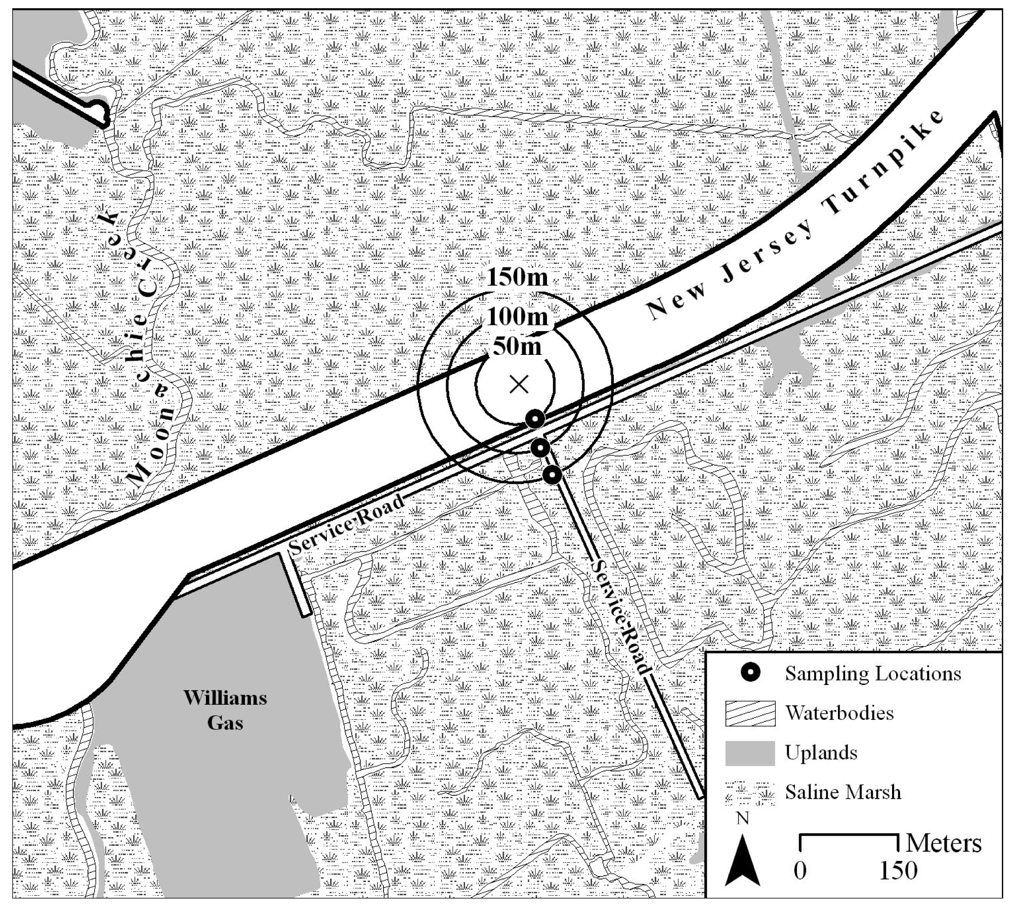
Traffic-related PAHs, TSP, and PM2.5 were monitored for one year in the immediate vicinity of the New Jersey Turnpike (NJTPK) (latitude/longitude: +40.817/−74.044) (Figure 1). The NJTPK is a major highway in the U.S. connecting the metropolitan areas of New York and Philadelphia with as many as ∼700,000 vehicles transiting this highway per day. The sampling location was considered to be a representative monitoring site for traffic-related air pollutants as no other anthropogenic emission sources are present within 800 m of the sampling site. In addition, the land on both the upwind and downwind sides of the highway is open flat marshlands. Therefore, we expect measurements from this sampling location to be strongly affected by traffic-related emissions, assuming that the contribution of other anthropogenic source emissions (residential heating, wood burning, industrial sources, etc.) is minimal.
Three secured sampling sites were selected in a south-eastern direction from the NJTPK at increasing distances of 50, 100, and 150 m from the center lane of the six-lane NJTPK. A maximum distance of 150 m was chosen based on many studies that have indicated PM concentrations to decline markedly within 150 m from major roadways [17,21,23]. Scaffolding platforms holding air quality monitoring equipment were installed at the three sites at highway level.
2.2. Ambient Air Sampling
The paired PAHs, TSP and PM2.5 samples were collected at the three sites simultaneously for 24 h (8:00 a.m. to 8:00 a.m. on the next day) on every sixth day starting 21 September 2007 and ending on 21 September 2008. Samples were retrieved immediately after samplings to avoid any evaporative losses of PAHs. At each site, sampling was performed at a height of 1.9 m above the platform and at least 2 m away from any obstruction.
Particulate-phase PAHs and TSP were collected on glass fiber filters (GFF; 20 × 25 cm, pore size 0.7 μm) and gas-phase PAHs were collected on two series of polyurethane foam (PUF) plugs (9.85 × 10 cm) by using Hi-vol. samplers (TE-PNY1123, Tisch Environmental, Inc., OH). Prior to sampling, GFF filters were prebaked at 550 °C for 24 h to eliminate organic species; PUF plugs were extracted with acetone and petroleum ether for 24 h and then dried in a vacuum desiccator and sealed in glass jars. Three Hi-vol. samplers were operated at a flow rate of 0.6∼0.8 m3/min, yielding individual sample volumes of 900∼1200 m3. A digital manometer was used to measure differential pressure (inches in H2O) as well as temperature and atmospheric pressure before and after each sampling for the flow meter conversions. After sampling, GFF and PUF samples were wrapped in aluminum foil and stored in baked clean glass jars, respectively, and stored in a freezer at −20 °C until extraction and analysis.
PM2.5 samples were captured onto Teflon filters (diameter = 47 mm, pore size = 2.0 μm; Whatman), by a Well Impactor Ninety Six (WINS) impactor with a 2.5 μm cut-point (Partisol-FRM Model 2000, Thermo Electron Corporation, MA). Three PM2.5 samplers were operated at a sampling flow rate of 16.7 L/min, resulting in a total sampled air volume of 24 m3 for each sample.
2.3. Sample Analysis
Eight nonvolatile PAHs (PAHs with more than 4 rings: MW 228–278) were selected as target compounds due to their abundance in traffic emissions and their adverse health effects observed in young children [5–8,24–26]. The eight PAHs monitored in this study were: benz[a]anthracene (BaA), chrysene (Chry), benzo[b]fluoranthene (BbFA), benzo[k]fluoranthene (BkFA), benzo[a]pyrene (BaP), indeno[1,2,3-c,d]pyrene (IP), dibenz[a,d]anthracene (DahA), and benzo[ghi]perylene (BghiP). PAHs were analyzed as the sum of gas and particulate phase since nonvolatile PAHs predominately exist in the particulate phase [27]. Detailed analytical protocols employed for the measurement of PAHs have been reported elsewhere [28] and a brief summary is given here. Prior to Soxhlet extraction, the GFF and PUF samples were treated with a known amount of deuterated compounds (chrysene-d10, and perylene-d12) as a surrogated standard for the recovery corrections. Then, filters and PUFs soxhlet extractions were analyzed for total PAHs (gas + particulate). The sample extracts were reduced to 0.5 mL by a rotary evaporator and cleaned via elution through alumina using hexane and a 2:1 mixture of DCM and hexane. The samples were then concentrated to approximately 200 μL under a gentle stream of high purity nitrogen and spiked with an internal standard made up of 2 deuterated compounds (anthracene-d10, and benz[a]anthracene-d10) prior to GC/MSD (Agilent 6890 N GC/5975MSD) analysis. A HP-5MS (30 m × 250 μm × 0.25 μm) capillary column (Agilent, Palo Alto, CA) was used with helium as a carrier gas. The temperature was programmed from 55 °C (1 min) to 320 °C at 125 °C min−1. 1 μL of the sample was introduced to an injector set at pulsed splitless mode. PAHs were quantified by GC/MSD using selective ion monitoring (SIM) and the method of internal standards.
The gravimetric analysis was performed for TSP and PM2.5 measurements by weighing the filters before and after sampling with a micro-balance at the Environmental and Occupational Health Sciences Institute (EOHSI), UMDNJ, NJ. The filters were equilibrated at a temperature of 20 °C and a relative humidity of 30–40% in the equilibrating room for 24 h before weighing.
2.4. Meteorological Parameters
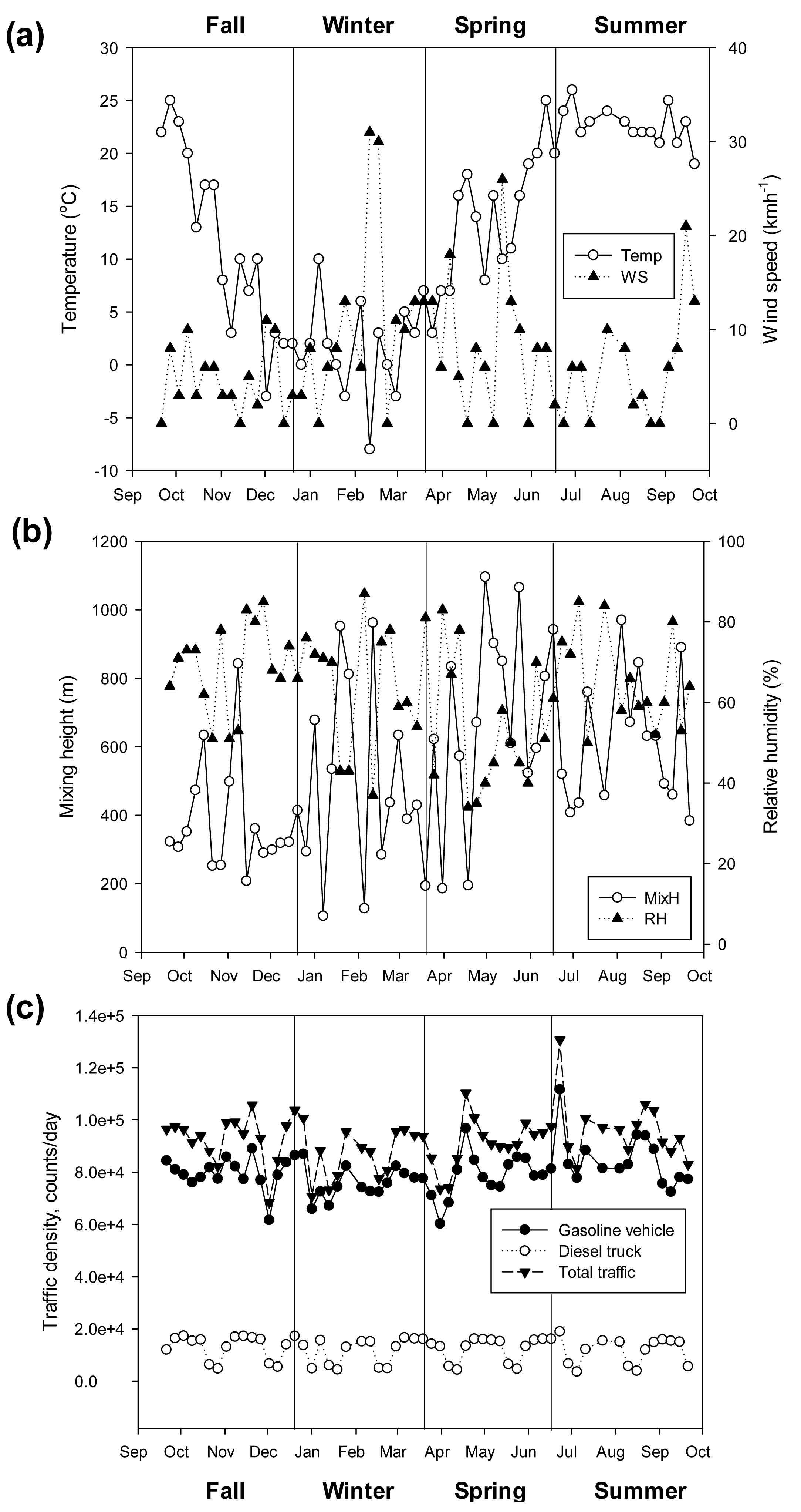
The meteorological data during the sampling periods were simultaneously collected from Teterboro airport, which is the closest weather station to the sampling location [29]. Hourly wind speed, wind direction, ambient temperature, precipitation, and humidity data were averaged according to our concurrent 24 h sampling period. Seasons were defined by solstices and equinoxes: fall (20 September–20 December), winter (21 December–19 March), spring (20 March–20 June), and summer (20 June–21 September). Daily weather circumstances (i.e., sunny, cloudy, or foggy conditions) were also obtained from the weather website as well as field records on the sampling day. Information on mixing height was obtained every 3 h during the sampling periods from the NOAA AIR Resources Laboratory archive [30]. Temporal variations of the meteorological parameters are presented in Figure 2 and the average meteorological conditions for each season were also summarized in supporting information (Table 1).
2.5. Traffic Counts
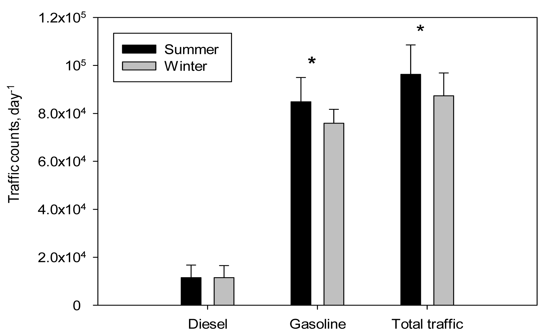
The 24-hour north and south bound traffic count, passing the sampling location between exit 16W–18W was obtained from the NJTPK Transportation Authority and divided into three categories: gasoline, diesel, and total traffic counts. Vehicle counts of class 1–3 were summed as a surrogate for gasoline traffic counts and the sum of class 4–6 and class B2–3 vehicle counts was used as a surrogate for diesel traffic [31]. Total traffic count was primarily dominated by gasoline-powered cars (∼85%) with a daily traffic density of 80,000 day−1 for gasoline powered cars and 12,000 day−1 for diesel powered trucks during the sampling periods. Temporal variations of daily traffic counts are presented in Figure 2. While diesel-powered vehicle volume were constant throughout the season, gasoline-powered vehicle and the total traffic volume increased significantly (10–12%) during the summer, when compared to the winter season (Figure 3).
2.6. Quality Control/Quality Assurance
A calibration of flow rate was performed every three months and after maintenance was done on the motor for the Hi-vol. sampler using a digital manometer and a calibration device (TE 5040 PUF Calibration Kit, Tisch Environ. Inc., Cleveland, OH, USA). Regular field, laboratory filter and PUF blanks were analyzed for any background contamination during sampling and transportation of samples to the laboratory. The mean recoveries of each spiked surrogate standard were above 60% for all compounds. The limit of detection (LODs) for each PAHs, defined as three times the standard deviation of the field blanks in filter and PUF, ranged from 0.001 to 0.022 ng/m3 based on the average sampling volume of 910 m3.
2.7. Statistical Analysis
Due to the non-normal distribution of PAHs, nonparametric analyses were conducted. PAH levels were analyzed as the sum of eight nonvolatile PAHs (Σ8PAHs). Wilcoxon Singed-ranks test were performed to compare levels at varying distances (50–100 m and 100–150 m; samples were taken from the three sites on the same days) from the highway for the effects of season and wind direction on horizontal gradient patterns. For the analysis, concentrations measured on different days were averaged by consistency in the three major wind directions on the day of measurement; upwind (SS, SE and EE), parallel (NE and SW), and downwind (NN, NW and WW). The frequency of the major wind direction, stratified by season, was presented in Table 1.
The effect of day-of-the-week variations on measured air pollutants and traffic counts were analyzed using the Mann-Whitney U test. Results were considered statistically significant if the p-value was less than 0.05. The data analysis was conducted using SPSS software (SPSS; Chicago, IL, version 17).
3. Results
3.1. Horizontal Gradient Patterns: Effects of Season
The annual average Σ8PAHs and TSP concentrations decreased significantly with increasing distance from the highway (Table 2, p < 0.05 and p < 0.001 for Σ8 PAHs and TSP, respectively; Wilcoxon Singed-ranks test). Spatial differences in Σ8PAHs and TSP concentrations from 50 m to 150 m from the highway ranged between 37% and 31%, respectively. Similarly, all of the individual PAH compounds decreased significantly from 50 m to 150 m from the highway (20–44% concentration decreases for BaP and DahA, respectively). In comparison, PM2.5 concentrations were not significantly different between the farthermost distances (100–150 m; p > 0.05) and very little decrease (2%) was observed within 150 m of the highway.
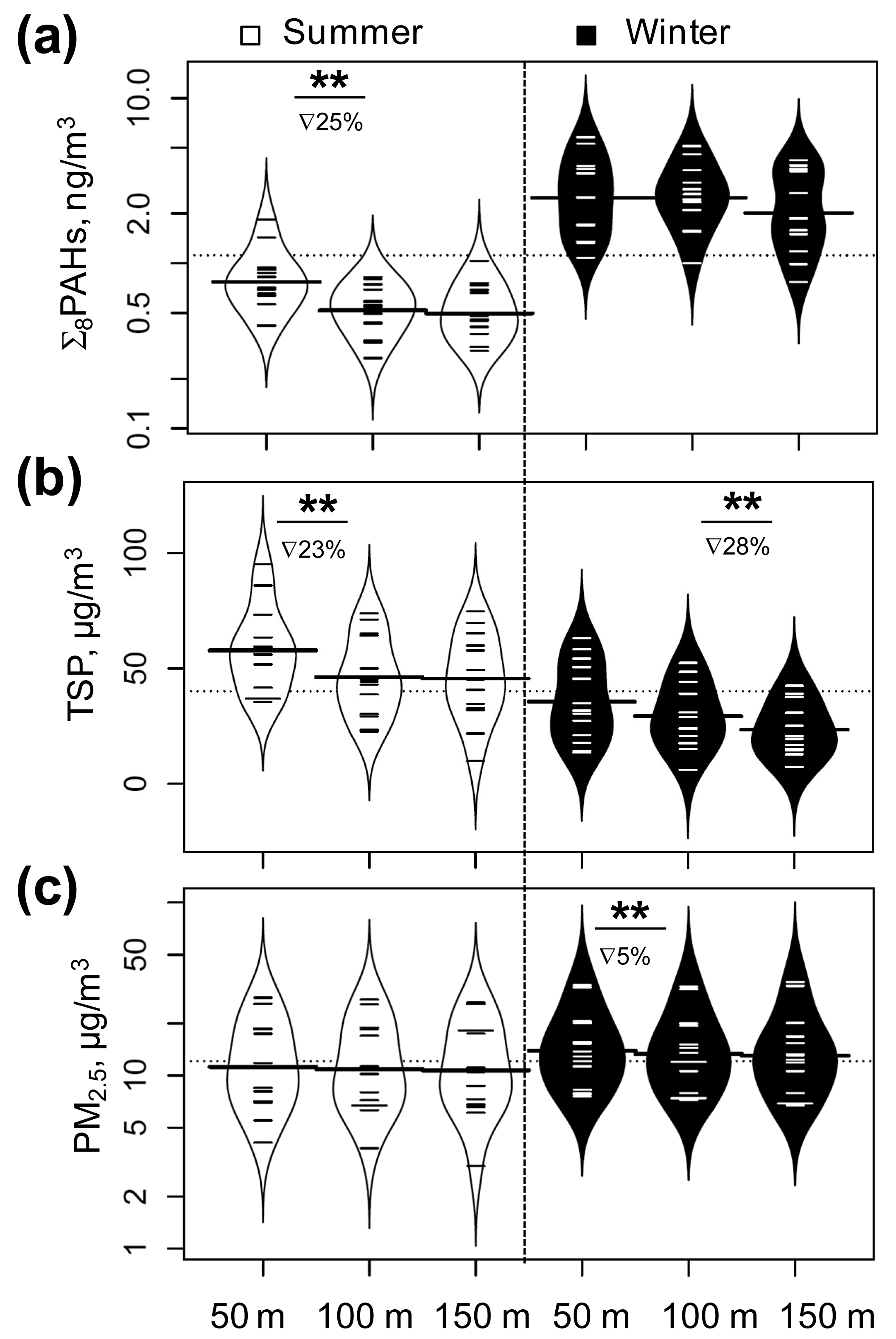
A distinct horizontal gradient pattern was observed for Σ8PAHs when data were analyzed by season (summer versus winter). During the summer, the average Σ8PAHs and TSP concentrations declined significantly between 50 and 100 m from the highway (Figure 4(a) and (b), 23% and 21% decrease for Σ8PAHs and TSP, respectively, p < 0.01; Wilcoxon Singed-ranks test). In the winter, Σ8PAHs decreased only between 100 and 150 m from the highway (26% decrease) whereas average TSP concentrations exhibited a persistently decreasing trend within 150 m of the highway (Figure 4(b)). A minimal yet significant decrease in PM2.5 concentrations was observed between 50 and 100 m from the highway in the winter (Figure 4(c), 4% decrease; p < 0.01), however, PM2.5 concentrations were not statistically different across all measured distances from the highway in the summer.
3.2. Effects of Wind Direction on the Horizontal Gradient Patterns
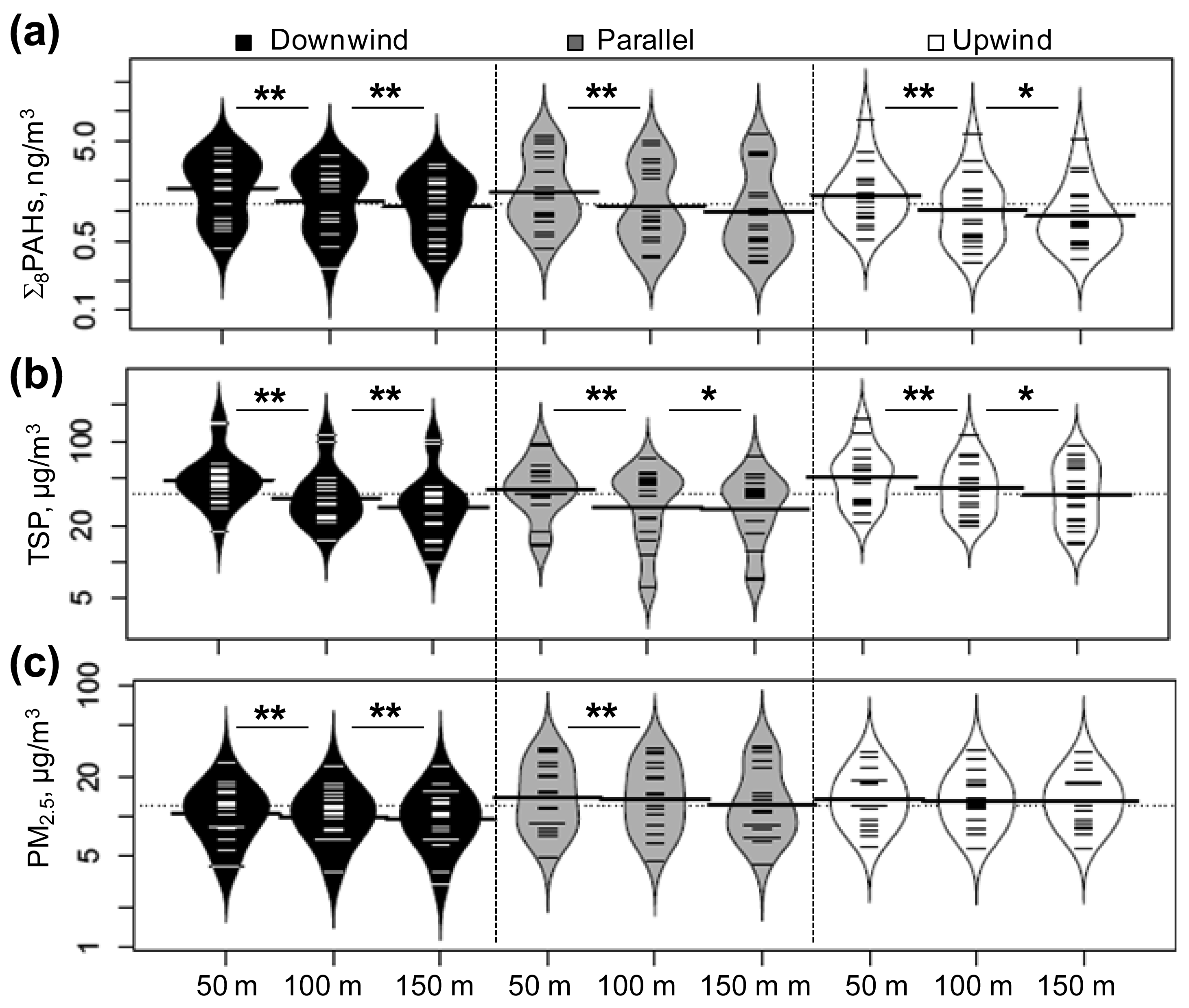
The decreasing trend of Σ8PAHs and TSP concentrations persisted within 100m from the highway regardless of wind directions (Figure 5(a) and (b), p < 0.05; Wilcoxon Singed-ranks test). The PM2.5 concentration gradient was most susceptible to wind direction; however, reductions in PM2.5 concentrations at increasing distance were minimal (Figure 5(c)).
Upwind condition compared to downwind was characterized by the substantially higher temperature and relative humidity but lower mixing height (Figure 6; Kruskal-Wallis test). However, there were no significant differences in wind speed and total traffic counts by wind direction.
3.3. The Ratios among Pollutants: Effects of Distance
The ratios of Σ8PAHs to PM2.5 decreased significantly with increasing distance from the highway (Table 3; p < 0.01; Wilcoxon Signed-ranks test), while the ratios Σ8PAHs to TSP did not vary significantly by distance (p > 0.05). In contrast, the ratios of PM2.5 to TSP increased significantly with increasing distance from the highway (p < 0.001).
3.4. Day-of-the-Week Variations
A significantly lower diesel traffic count, but not gasoline traffic count, was observed during weekends versus weekdays, representing only 35% of weekday diesel traffic counts (Table 4, p < 0.01, Mann-Whitney U test). Σ8PAHs and TSP, but not PM2.5, concentrations measured on weekends were 12–37% lower than those on weekdays, respectively, corresponding to lower diesel traffic volume.
3.5. Temporal Variations in PAHs, TSP and PM2.5 Concentrations
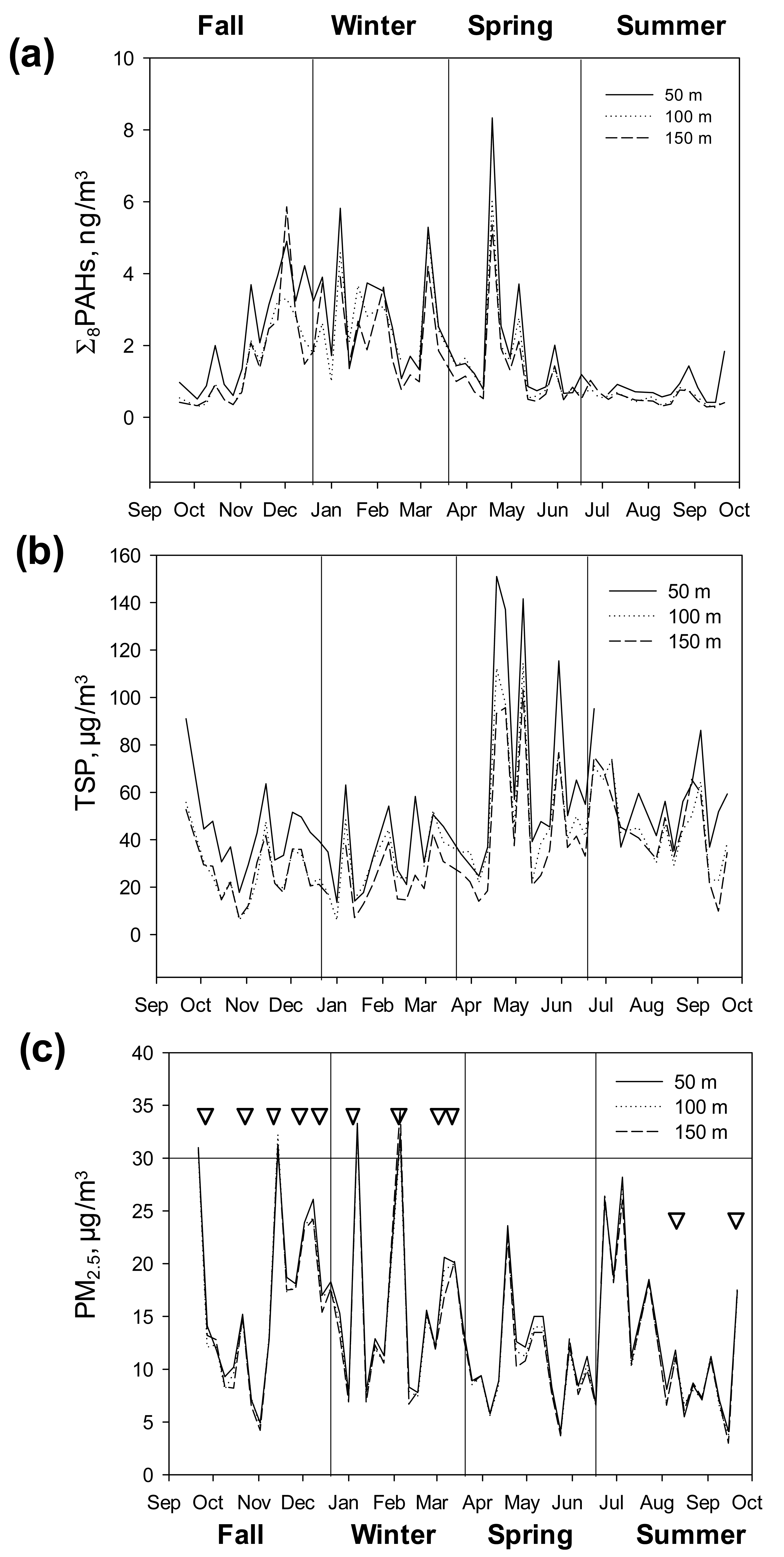
Elevated Σ8PAHs levels were observed in cold months (December–March) and occasional spikes were found in May, 2008 (Figure 7(a)). During spring season, the highest TSP concentration was observed due to the presence of pollen particles, as noted by yellow filter color at the time of takedown (Figure 7(b)). PM2.5 showed strong day-to-day variations throughout the sampling periods (Figure 7(c)). For example, PM2.5 concentrations over 30 μg/m3 were observed on 9/21/07, 11/14/07, 1/7/08, and 2/5/08. On each of these sampling dates, the ambient weather condition was characterized by foggy air (indicated by “∇” symbol in Figure 7(c)), corresponding to lower mixing height and wind speed compared to non-foggy days (Table 5). On foggy days, the levels of Σ8PAHsand PM2.5, but not TSP, were 1.5–2 times higher than those measured on non-foggy days.
4. Discussion
Our main objective was to determine the effects of season on horizontal gradients of trafficgenerated PAHs, TSP and PM2.5 concentrations within 150 m of the highway. We found that PAHs and TSP concentrations decreased substantially with increasing distance from the highway and the horizontal gradient patterns of Σ8PAHs varied by season. Further, the levels of Σ8PAHs and TSP, but not PM2.5, measured on weekdays were higher than those on weekends.
The overall horizontal gradient patterns of Σ8PAHs and TSP were similar, possibly due to the fact that particulate PAHs were measured in TSP. Additionally, they showed similar day-of-the-week variations with a good reflection of diesel traffic activity. Weekends compared to weekdays were associated with lower levels of Σ8PAHs and TSP, corresponding to a 64% decrease in diesel traffic volume. High-speeded vehicles on highways can generate not only combustion emissions but also non-combustion emissions such as re-suspended road dust, tire debris, and brake wear. Assuming traffic counts are a proxy to re-suspension of road dust particles, and that diesel-powered vehicles have a greater impact on re-suspension of particles than gasoline-powered vehicles, three-fold higher diesel traffics during weekdays compared to weekends may be responsible for elevated levels of TSP as well as TSP-associated PAHs. Furthermore, the higher Σ8PAHs concentrations may also be attributed to the higher amounts of PAHs in diesel fuels than in gasoline-based fuel, thus they can be emitted to a greater extent from diesel-powered trucks than gasoline-powered vehicles [12].
Distinct seasonal gradient patterns of Σ8PAHs were observed in this study. A significant concentration decrease in Σ8PAHs was only found between the closest distances (50–100 m) in the summer but between the furthermost distances (100–150 m) in the winter. The result indicates that Σ8PAHs may be transported further down from the highway in winter. Zhu and colleagues [32] also reported slower decay rates of UFP concentrations within 300 m of highways in winter than in summer, due to a weaker atmospheric dispersion effect in winter. Beyer et al. calculated travel distance of PAHs for summer and winter, as the function of temperature, chemical reaction with atmospheric oxidants, and deposition/adsorption rate onto surface of existing particles. They reported that PAHs can travel up to six times farther in winter than in summer due to: (1) a reduced potential for chemical/photochemical reactions with ozone or OH radicals [33,34]; (2) a weaker dispersion/mixing condition; and (3) stronger adsorption onto particle surfaces at lower temperature [35]. In comparison, TSP concentration dissipated the most within 100 m of the highway regardless of season or wind direction, indicating that gravitational settling, rather than air dilution or deposition on surfaces due to diffusion and turbulence motion, is an important particle removal/loss process for TSP within this distance [17,36,37].
The overall horizontal gradient of PM2.5 within 150 m was very weak compared to Σ8PAHs and TSP. The little spatial variations of PM2.5 and lack of day-of-the-week variations may indicate that the contribution of regional sources (i.e., coal-fired power plants, heating sources, residual oil combustion, and motor vehicles) and long-range transport of PM2.5 may outweigh the contribution of primary traffic emissions, masking the effects of the highway [38]. The lack of a concentration gradient in PM2.5 was also seen vertically in residential outdoor air in New York City (NYC) [39], supporting the idea of large contributions from long-range transported aerosols and regional sources in NYC and northeastern U.S. cities [38]. Significant decrease in ratios of Σ8PAHs to PM2.5 or increase in ratios of PM2.5 to TSP by increasing distance may further support this explanation. While it was not our main study objective, we observed several important factors affecting measured air pollutant levels. For one, occasional high Σ8PAHs peaks were also observed on each of the high pollen days, corresponding to high TSP peaks (Figure 6). This might be due to increased adsorption capacity of particulate and gaseous PAHs onto a large surface area of pollen particles collected on TSP [40]. PM2.5 concentrations were not affected by the presence of dispersed pollen particles since pollen particles are generally greater than 40 μm in size. On the other hand, foggy days, concurrent with lower mixing heights and wind speed, were identified as an important parameter: under these conditions, the measured air pollutant levels may be even greater due to restrained mixing conditions. This can be also explained by the role of fog droplets. They can serve as an efficient carrier of particulate and gas-phase pollutants due to an enhanced particle scavenging effect through the nucleating and collision process [41,42], possibly resulting in higher levels of PM2.5 and Σ8PAHs in foggy days. This was further supported by significant and moderate correlations between Σ8PAHs and PM2.5 (Data not shown).
As shown in many studies, the measured concentrations were expected to be higher for the downwind than for the upwind measurement [21]. Consistent with other studies, we also observed the higher levels of Σ8PAHs, when wind blew from the highway. The results indicate that traffic emission is the major source of PAHs. Lower upwind Σ8PAHs concentrations could also be attributed to the fact that most upwind samples (37%) were collected in the summer when Σ8PAHs concentrations are expected to be lower due to: (1) reduced emission sources (e.g., heating emission sources) [34]; (2) elevated loss mechanisms by atmospheric photochemical/chemical reactions [33,34]; and (3) non-preferential particle phase partitioning at higher temperatures. Indeed, upwind compared to downwind conditions were associated with higher temperature and humidity, typically seen in summer. Similarly, we also found seasonal effect on TSP concentrations. Higher levels of TSP measured in upwind conditions may also be due to the elevated TSP concentrations in the summer (Figure 4(b)). In comparison, higher upwind PM2.5 concentrations, compared to downwind, are not likely to be explained by seasonal effect since PM2.5 concentrations were lower in the summer than in the winter. Higher upwind PM2.5 concentrations may imply that there are high background levels of PM2.5 from upwind, which may outweigh the highway contribution.
We acknowledge several limitations to this study. A typical traffic tracer such as BC was not measured in this study. However, the use of PAH diagnostic ratios in this study identified traffic emission as a major PAH sources at this site (data not shown). Another limitation was the inability to monitor at a longer distance (i.e., 300 m) from the highway due to limited accessibility to power supply. This would have allowed us to better understand the horizontal gradients of highway-generated air pollutants especially during the winter when they could travel farther away from the highway. While most PAHs are mainly associated with fine particles [43], PAHs associated with PM2.5 were not measured in the study. Comparisons between PAHs associated with TSP and PM2.5 could give us a better understanding of size-dependence transportation of PAHs generated from the highway.
5. Conclusions
A strength of our study is that sampling was conducted at a secluded highway where traffic emissions are the major representative source of PAHs and TSP, and therefore the true effect of the highway can be seen within the sampling distance. We found that the ambient levels of highway-generated Σ8PAHs, TSP and PM2.5 are a function of the proximity to the highway, variations in meteorological parameters, and day-of-the-week variations. Distinct seasonal gradient patterns of Σ8PAHs further highlight the importance of travel distance and the potential long-range transport of PAHs in winter.


| Season | Temp. (°C) | R.H. (%) | Preci. (cm) | W.S. (km/h) | M.H. (m) | Wind direction a Frequency (%) | ||
|---|---|---|---|---|---|---|---|---|
| U | D | P | ||||||
| Fall (n = 16) | 11.2 ±8.7 | 68.6 ± 10.7 | 0.52 ± 1.02 | 4.56 ± 3.63 | 384.3 ± 162.4 | 5 (31) | 5 (31) | 6 (38) |
| Winter (n = 14) | 1.71 ±4.6 | 64.7 ± 15.6 | 0.45 ± 0.75 | 10.9 ± 9.40 | 488.3 ± 285.8 | 3 (21) | 4 (29) | 7 (50) |
| Spring (n = 15) | 14.0 ±6.1 | 53.3 ± 15.5 | 0.14 ± 0.30 | 8.2 ±7.18 | 698.1 ± 271.8 | 4 (27) | 7 (47) | 4 (27) |
| Summer (n = 14) | 22.6 ±1.8 | 65.6 ± 11.8 | 0.47 ± 0.98 | 5.92 ± 5.99 | 611.4 ± 192.3 | 7 (50) | 3 (21) | 4 (29) |
Note: Data presented as mean ± standard deviation. Temp. (Temperature), R.H. (Relative Humidity), Preci. (Precipitation), W.S. (Wind Speed), M.H. (Mixing Height).
afrequency of the major wind direction: U (upwind) was defined if the major wind direction on each sampling day was from SS, SE, and EE; D (downwind) by NN, NW, and WW, and P (parallel) by NE and SW.| Analyte | Abbr. | LOD | 50 m (n = 56) | 100 m (n = 56) | a 50–100 m | 150 m (n = 56) | b100–150 m | |||
|---|---|---|---|---|---|---|---|---|---|---|
| ng/m3 | Median | Avg ± SD | Median | Avg ± SD | p | Median | Avg ± SD | p | ||
| Benz[a]anthracene | BaA | 0.001 | 0.09 | 0.12 ± 0.10 | 0.05 | 0.09 ± 0.08 | *** | 0.05 | 0.08 ± 0.08 | *** |
| Chrysene | Chry | 0.001 | 0.23 | 0.32 ± 0.21 | 0.19 | 0.24 ± 0.15 | *** | 0.16 | 0.21 ± 0.15 | *** |
| Benzo[b]fluoranthrene | BbFA | 0.001 | 0.16 | 0.21 ± 0.14 | 0.11 | 0.15 ± 0.11 | *** | 0.10 | 0.14 ± 0.10 | |
| Benzo[k]fluoranthrene | BkFA | 0.002 | 0.13 | 0.18 ± 0.13 | 0.10 | 0.13 ± 0.09 | *** | 0.09 | 0.13 ± 0.10 | * |
| Benzo[a]pyrene | BaP | 0.001 | 0.12 | 0.18 ± 0.15 | 0.09 | 0.14 ± 0.11 | *** | 0.08 | 0.13 ± 0.13 | *** |
| Indeno[c,d]pyrene | IP | 0.010 | 0.23 | 0.33 ± 0.32 | 0.16 | 0.26 ± 0.27 | *** | 0.15 | 0.24 ± 0.26 | *** |
| Dibenz[a,h]anthracene | DahA | 0.022 | 0.05 | 0.10 ± 0.15 | 0.04 | 0.07 ± 0.08 | *** | 0.04 | 0.06 ± 0.06 | ** |
| Benzo[ghi]perylene | BghiP | 0.005 | 0.36 | 0.57 ± 0.60 | 0.23 | 0.47 ± 0.48 | *** | 0.23 | 0.41 ± 0.46 | *** |
| c Σ8PAHs | NA | NA | 1.40 | 2.00 ± 1.61 | 0.97 | 1.54 ± 1.29 | *** | 0.88 | 1.41 ± 1.29 | *** |
| TSP | NA | NA | 45.5 | 51.7 ± 29.6 | 34.9 | 39.3 ± 23.2 | *** | 31.4 | 35.6 ± 22.2 | *** |
| PM2.5 | NA | NA | 12.1 | 14.1 ± 7.5 | 11.8 | 13.7 ± 7.4 | *** | 11.9 | 13.5 ± 7.6 | |
Note: Data presented as median with arithmetric mean ± standard deviation; Unit expressed in ng/m3 for PAHs and μg/m3 for TSP and PM2.5; p-value
aWilcoxon Singed-ranks testperformed between 50 m and 100 m; significance at * p < 0.05, ** p < 0.01, and *** p < 0.001; p-valuebWilcoxon Singed-ranks test performed between 100 m and 150 m; significance at * p < 0.05, ** p < 0.01, and *** p < 0.001;cΣ8PAHs : BaA, Chry, BbFA, BkFA, BaP, IP, DahA, and BghiP.| Ratio | 50 m (n = 56) | 100 m (n = 56) | 150 m (n = 56) | b (50–100 m) p | b (100–150 m) p |
|---|---|---|---|---|---|
| a Σ8PAHs/TSP | 30.2 | 29.5 | 32.2 | 0.067 | 0.639 |
| a Σ8PAHs/PM2.5 | 131.7 | 105.4 | 96.8 | *** | ** |
| PM2.5/TSP | 0.30 | 0.35 | 0.43 | *** | *** |
aMedian ratio (×1000) presented;bWilcoxon Singed-ranks test conducted for the differences between distances; Significance at * p < 0.05, ** p < 0.01, and *** p < 0.001.
| Variables | Weekdays (n = 40) | Weekends (n = 16) | WD/WK a |
|---|---|---|---|
| Total traffic | 95579 (95701 ± 9169) | 82988 (83196 ± 7447) | 1.2 ** |
| Diesel | 15505 (14996 ± 2242) | 5461 (5345 ± 971) | 2.8 ** |
| Gasoline | 79323 (80706 ± 8435) | 77808 (77852 ± 7713) | 1.0 |
| Σ8PAHs b | 1.59 (2.21 ± 1.73) | 1.00 (1.48 ± 1.18) | 1.6 |
| TSP b | 46.7 (56.3 ± 32.2) | 41.2 (40.4 ± 17.7) | 1.1 |
| PM2.5 b | 12.1 (14.5 ± 7.49) | 11.8 (13.2 ± 7.50) | 1.0 |
Note: WD/WK
ais the ratio of the median levels of pollutant measured in weekdays to weekends; Data presented as median with (arithmetric mean ± standard deviation). Mann-Whitney U test performed for the differences between weekdays and weekends; ** p-value < 0.01; Unit expressed in ng/m3 for Σ8PAHs and μg/m3 for TSP and PM2.5.bdata presented air pollutant levels measured at 50 m from the highway; Σ8PAHs includes BaA, Chry, BbFA, BkFA, BaP, IP, DahA, and BghiP.| Meteorological parameters/pollution | Foggy days (n = 11) | Non-foggy days (n = 45) | FG/NFG a |
|---|---|---|---|
| Temperature (°C) | 10.0 (11.9 ± 6.90) | 15.0 (12.5 ± 9.91) | 0.67 |
| Relative Humidity (%) | 66.0 (69.6 ± 12.6) | 61.5 (61.6 ± 14.5) | 1.1 |
| Wind speed (m/s) | 5.0 (5.18 ± 4.98) | 6.0 (7.79 ± 7.38) | 0.8 |
| Mixing height (m) | 323 (322 ± 157) | 585 (593 ± 250) | 0.6 ** |
| Σ8PAHs b | 2.52 (2.78 ± 1.75) | 1.33 (1.80 ± 1.54) | 1.7 |
| TSP b | 54.2 (53.2 ± 17.0) | 43.1 (51.4 ± 32.1) | 1.3 |
| PM2.5 b | 20.1 (22.7 ± 7.66) | 11.2 (12.2 ± 5.93) | 1.8 ** |
Note: FG/NFG
ais the ratio of the median levels of pollutant measured in foggy days to non-foggy days; Data presented as median with (arithmetric mean ± standard deviation); Mann-Whitney U test performed for the differences between foggy days and non-foggy days; ** p-value < 0.001; Unit expressed in ng/m3 for Σ8PAHs and μg/m3 for TSP and PM2.5;bdata presented air pollutant levels measured at 50 m from the highway; Σ8PAHs includes BaA, Chry, BbFA, BkFA, BaP, IP, DahA, and BghiP.Acknowledgments
The authors are thankful to Joe Grzyb, Edward Konsevick, Joseph Sarnoski, Yena Jun, Amish Shah, and Angela Kwok, for assisting with the field work and chemical analysis and as well as Christine Hobble and Erika Baldino for proof reading this manuscript. We also thank the New Jersey Turnpike Transportation Authority for providing highway traffic data. The study was made possible with the cooperation of Williams Gas Company that provided access and spaces for measurement stations. This project was supported by the Environmental Protection Agency project “Monitoring of Air Toxic Particulate Pollutants from Heavily Trafficked New Jersey Turnpike: An Urban Community-Wide Project” (Grant NO. EPA-454/R-01-007).
References and Notes
- McConnell, R.; Berhane, K.; Yao, L.; Jerrett, M.; Lurmann, F.; Gilliland, F.; Künzli, N.; Gauderman, J. Traffic, susceptibility, and childhood asthma. Environ. Health Perspect. 2006, 114, 766. [Google Scholar]
- Pope, C.A.; Burnett, R.T.; Thun, M.J.; Calle, E.E.; Krewski, D.; Ito, K.; Thurston, G.D. Lung cancer, cardiopulmonary mortality, and long-term exposure to fine particulate air pollution. J. Am. Med. Assoc. 2002, 287, 1132–1141. [Google Scholar]
- Pope, C., III; Dockery, D. Health effects of fine particulate air pollution: Lines that connect. J. Air Waste Manag. Assoc. 2006, 56, 709–742. [Google Scholar]
- Miller, R.; Garfinkel, R.; Horton, M.; Camann, D.; Perera, F.; Whyatt, R.; Kinney, P. Polycyclic aromatic hydrocarbons, environmental tobacco smoke, and respiratory symptoms in an inner-city birth cohort. Chest 2004, 126, 1071–1078. [Google Scholar]
- Perera, F.P.; Rauh, V.; Whyatt, R.M.; Tsai, W.Y.; Tang, D.; Diaz, D.; Hoepner, L.; Barr, D.; Tu, Y.H.; Camann, D.; et al. Effect of prenatal exposure to airborne polycyclic aromatic hydrocarbons on neurodevelopment in the first 3 years of life among inner-city children. Environ. Health Perspect. 2006, 114, 1287–1292. [Google Scholar]
- Jedrychowski, W.; Galas, A.; Pac, A.; Flak, E.; Camman, D.; Rauh, V.; Perera, F. Prenatal ambient air exposure to polycyclic aromatic hydrocarbons and the occurrence of respiratory symptoms over the first year of life. Eur. J. Epidemiol. 2005, 20, 775–782. [Google Scholar]
- Jedrychowski, W.; Perera, F.; Maugeri, U.; Mrozek Budzyn, D.; Mroz, E.; Klimaszewska-Rembiasz, M.; Flak, E.; Edwards, S.; Spengler, J.; Jacek, R. Intrauterine exposure to polycyclic aromatic hydrocarbons, fine particulate matter and early wheeze. Prospective birth cohort study in 4 year olds. Pediatr. Allergy Immunol. 2010, 21, e723–e732. [Google Scholar]
- Jung, K.H.; Yan, B.; Chillrud, S.N.; Perera, F.P.; Whyatt, R.; Camann, D.; Kinney, P.L.; Miller, R.L. Assessment of Benzo[a]pyrene-equivalent Carcinogenicity and Mutagenicity of Residential Indoor versus Outdoor Polycyclic Aromatic Hydrocarbons Exposing Young Children in New York City. Int. J. Environ. Res. Public Health 2010, 7, 1889–1900. [Google Scholar]
- Bjorseth, A.; Ramdahl, T. Handbook of Polycyclic Aromatic Hydrocarbons: Emission Sources and Recent Progress in Analytical Chemistry; Marcel Dekker: New York, NY, USA, 1985. [Google Scholar]
- Miguel, A.; Kirchstetter, T.; Harley, R.; Hering, S. On-road emissions of particulate polycyclic aromatic hydrocarbons and black carbon from gasoline and diesel vehicles. Environ. Sci. Technol. 1998, 32, 450–455. [Google Scholar]
- Rogge, W.; Hildemann, L.; Mazurek, M.; Cass, G.; Simoneit, B. Sources of fine organic aerosol. 2. Noncatalyst and catalyst-equipped automobiles and heavy-duty diesel trucks. Environ. Sci. Technol. 1993, 27, 636–651. [Google Scholar]
- Lee, W.; Wang, Y.; Lin, T.; Chen, Y.; Lin, W.; Ku, C.; Cheng, J. PAH characteristics in the ambient air of traffic-source. Sci. Total Environ. 1995, 159, 185–200. [Google Scholar]
- Yang, S.Y.N.; Connell, D.; Hawker, D.; Kayal, S. Polycyclic aromatic hydrocarbons in air, soil and vegetation in the vicinity of an urban roadway. Sci. Total Environ. 1991, 102, 229–240. [Google Scholar]
- Kojima, Y.; Inazu, K.; Hisamatsu, Y.; Okochi, H.; Baba, T.; Nagoya, T. Influence of secondary formation on atmospheric occurrences of oxygenated polycyclic aromatic hydrocarbons in airborne particles. Atmos. Environ. 2010, 44, 2873–2880. [Google Scholar]
- Fischer, P.; Hoek, G.; Van Reeuwijk, H.; Briggs, D.; Lebret, E.; Van Wijnen, J.; Kingham, S.; Elliott, P. Traffic-related differences in outdoor and indoor concentrations of particles and volatile organic compounds in Amsterdam. Atmos. Environ. 2000, 34, 3713–3722. [Google Scholar]
- Clements, A.L.; Jia, Y.; Denbleyker, A.; McDonald-Buller, E.; Fraser, M.P.; Allen, D.T.; Collins, D.R.; Michel, E.; Pudota, J.; Sullivan, D. Air pollutant concentrations near three Texas roadways, part II: Chemical characterization and transformation of pollutants. Atmos. Environ. 2009, 43, 4523–4534. [Google Scholar]
- Zhu, Y.; Hinds, W.; Kim, S.; Sioutas, C. Concentration and size distribution of ultrafine particles near a major highway. J. Air Waste Manag. Assoc. 2002, 52, 1032–1042. [Google Scholar]
- Zhu, Y.; Hinds, W.; Kim, S.; Shen, S.; Sioutas, C. Study of ultrafine particles near a major highway with heavy-duty diesel traffic. Atmos. Environ. 2002, 36, 4323–4335. [Google Scholar]
- Reponen, T.; Grinshpun, S.; Trakumas, S.; Martuzevicius, D.; Wang, Z.; LeMasters, G.; Lockey, J.; Biswas, P. Concentration gradient patterns of aerosol particles near interstate highways in the Greater Cincinnati airshed. J. Environ. Monit. 2003, 5, 557–562. [Google Scholar]
- Tiitta, P.; Raunemaa, T.; Tissari, J.; Yli-Tuomi, T.; Leskinen, A.; Kukkonen, J.; Härkönen, J.; Karppinen, A. Measurements and modelling of PM2.5 concentrations near a major road in Kuopio, Finland. Atmos. Environ. 2002, 36, 4057–4068. [Google Scholar]
- Hitchins, J.; Morawska, L.; Wolff, R.; Gilbert, D. Concentrations of submicrometre particles from vehicle emissions near a major road. Atmos. Environ. 2000, 34, 51–59. [Google Scholar]
- Berico, M.; Luciani, A.; Formignani, M. Atmospheric aerosol in an urban area—Measurements of TSP and PM10 standards and pulmonary deposition assessments. Atmos. Environ. 1997, 31, 3659–3665. [Google Scholar]
- Morawska, L.; Thomas, S.; Gilbert, D.; Greenaway, C.; Rijnders, E. A study of the horizontal and vertical profile of submicrometer particles in relation to a busy road. Atmos. Environ. 1999, 33, 1261–1274. [Google Scholar]
- Miller, R.L.; Garfinkel, R.; Horton, M.; Camann, D.; Perera, F.P.; Whyatt, R.M.; Kinney, P.L. Polycyclic aromatic hydrocarbons, environmental tobacco smoke, and respiratory symptoms in an inner-city birth cohort. Chest 2004, 126, 1071–1078. [Google Scholar]
- Boffetta, P. Cancer risk from occupational and environmental exposure to polycylic aromatic hydrocarbons. Cancer Causes Control 1997, 8, 442–472. [Google Scholar]
- Perera, F.; Li, Z.; Whyatt, R.; Hoepner, L.; Wang, S.; Camann, D.; Rauh, V. Prenatal airborne polycyclic aromatic hydrocarbon exposure and child IQ at age 5 years. Pediatrics 2009, 124, e195–e202. [Google Scholar]
- Baek, S.; Goldstone, M.; Kirk, P.; Lester, J.; Perry, R. Phase distribution and particle size dependency of polycyclic aromatic hydrocarbons in the urban atmosphere. Chemosphere 1991, 22, 503–520. [Google Scholar]
- Naumova, Y.; Eisenreich, S.; Turpin, B.; Weisel, C.; Morandi, M.; Colome, S.; Totten, L.; Stock, T.; Winer, A.; Alimokhtari, S. Polycyclic aromatic hydrocarbons in the indoor and outdoor air of three cities in the US. Environ. Sci. Technol. 2002, 36, 2552–2559. [Google Scholar]
- Weather Underground. Available online: http://www.wunderground.com/history/ (accessed on 22 September 2008).
- Air Resources Laboratory. Available online: http://ready.arl.noaa.gov/READYcmet.php (accessed on 20 January 2009).
- New Jersey Turnpike Authority. Available online: http://www.state.nj.us/turnpike/toll-rates.html#classes (accessed on 28 January 2009).
- Zhu, Y.; Hinds, W.; Shen, S.; Sioutas, C. Seasonal and Spatial Trends in Fine Particulate Matter. Aerosol Sci. Technol. 2004, 38, 5–13. [Google Scholar]
- Schauer, C.; Niessner, R.; Pöschl, U. Polycyclic aromatic hydrocarbons in urban air particulate matter: Decadal and seasonal trends, chemical degradation, and sampling artifacts. Environ. Sci. Technol. 2003, 37, 2861–2868. [Google Scholar]
- Jung, K.H.; Patel, M.M.; Moors, K.; Kinney, P.L.; Chillrud, S.N.; Whyatt, R.; Hoepner, L.; Garfinkel, R.; Yan, B. Effects of heating season on residential indoor and outdoor polycyclic aromatic hydrocarbons, black carbon, and particulate matter in an urban birth cohort. Atmos. Environ. 2010, 44, 4545–4552. [Google Scholar]
- Beyer, A.; Wania, F.; Gouin, T.; Mackay, D.; Matthies, M. Temperature dependence of the characteristic travel distance. Environ. Sci. Technol. 2003, 37, 766–771. [Google Scholar]
- Hinds, W. Aerosol Technology: Properties, Behavior, and Measurement of Airborne Particles, 2nd ed.; Wiley-Interscience: Hoboken, NJ, USA, 1982. [Google Scholar]
- Sarnat, S.; Coull, B.; Ruiz, P.; Koutrakis, P.; Suh, H. The influences of ambient particle composition and size on particle infiltration in Los Angeles, CA, residences. J. Air Waste Manag. Assoc. 2006, 56, 186–196. [Google Scholar]
- Qin, Y.; Kim, E.; Hopke, P. The concentrations and sources of PM2.5 in metropolitan New York City. Atmos. Environ. 2006, 40, 312–332. [Google Scholar]
- Jung, K.H.; Bernabé, K.; Moors, K.; Yan, B.; Chillrud, S.N.; Whyatt, R.; Camann, D.; Kinney, P.L.; Perera, F.P.; Miller, R.L. Effects of floor level and building type on residential levels of outdoor and indoor polycyclic aromatic hydrocarbons, black carbon, and particulate matter in New York City. Atmosphere 2011, 2, 96–109. [Google Scholar]
- Okuyama, Y.; Matsumoto, K.; Okochi, H.; Igawa, M. Adsorption of air pollutants on the grain surface of Japanese cedar pollen. Atmos. Environ. 2007, 41, 253–260. [Google Scholar]
- Halsall, C.; Coleman, P.; Davis, B.; Burnett, V.; Waterhouse, K.; Harding-Jones, P.; Jones, K. Polycyclic aromatic hydrocarbons in UK urban air. Environ. Sci. Technol. 1994, 28, 2380–2386. [Google Scholar]
- Czuczwa, J.; Katona, V.; Pitts, G.; Zimmerman, M.; DeRoos, F.; Capel, P.; Giger, W. Analysis of fog samples for PCDD and PCDF. Chemosphere 1989, 18, 847–850. [Google Scholar]
- Bi, X.; Sheng, G.; Peng, P.; Chen, Y.; Fu, J. Size distribution of n-alkanes and polycyclic aromatic hydrocarbons (PAHs) in urban and rural atmospheres of Guangzhou, China. Atmos. Environ. 2005, 39, 477–487. [Google Scholar]
© 2011 by the authors; licensee MDPI, Basel, Switzerland. This article is an open access article distributed under the terms and conditions of the Creative Commons Attribution license (http://creativecommons.org/licenses/by/3.0/).
Share and Cite
Jung, K.H.; Artigas, F.; Shin, J.Y. Seasonal Gradient Patterns of Polycyclic Aromatic Hydrocarbons and Particulate Matter Concentrations near a Highway. Atmosphere 2011, 2, 533-552. https://doi.org/10.3390/atmos2030533
Jung KH, Artigas F, Shin JY. Seasonal Gradient Patterns of Polycyclic Aromatic Hydrocarbons and Particulate Matter Concentrations near a Highway. Atmosphere. 2011; 2(3):533-552. https://doi.org/10.3390/atmos2030533
Chicago/Turabian StyleJung, Kyung Hwa, Francisco Artigas, and Jin Y. Shin. 2011. "Seasonal Gradient Patterns of Polycyclic Aromatic Hydrocarbons and Particulate Matter Concentrations near a Highway" Atmosphere 2, no. 3: 533-552. https://doi.org/10.3390/atmos2030533
APA StyleJung, K. H., Artigas, F., & Shin, J. Y. (2011). Seasonal Gradient Patterns of Polycyclic Aromatic Hydrocarbons and Particulate Matter Concentrations near a Highway. Atmosphere, 2(3), 533-552. https://doi.org/10.3390/atmos2030533